A surface of degree 24 with 1 ​440 singularities of type $D_{4}$

Abstract

Using the invariant algebra of the complex reflection group denoted by $G_{32}$ in the Shephard–Todd classification, we construct three irreducible surfaces in ${\mathbf{P}}^{3}({\mathbb{C}})$ with many singularities: one of them has degree $24$ and contains $1~{}\!440$ quotient singularities of type $D_{4}$.

Let $\mu_{D_{4}}(d)$ denote the maximal number of quotient singularities of type $D_{4}$ that an irreducible projective surface of degree $d$ in ${\mathbf{P}}^{3}({\mathbb{C}})$ might have. Miyaoka [Miy] proved that

$$\mu_{D_{4}}(d)\hskip 1.00006pt\mathop{\leqslant}\nolimits\hskip 1.00006pt\frac{16}{117}d(d-1)^{2}.$$

For $d=8$, $16$ or $24$, this reads

$$\mu_{D_{4}}(8)\hskip 1.00006pt\mathop{\leqslant}\nolimits\hskip 1.00006pt53,\qquad\mu_{D_{4}}(16)\hskip 1.00006pt\mathop{\leqslant}\nolimits\hskip 1.00006pt492\qquad\text{and}\qquad\mu_{D_{4}}(24)\hskip 1.00006pt\mathop{\leqslant}\nolimits\hskip 1.00006pt1736.$$

The main results of this note are that

$$\mu_{D_{4}}(8)\hskip 1.00006pt\mathop{\geqslant}\nolimits\hskip 1.00006pt44,\qquad\mu_{D_{4}}(16)\hskip 1.00006pt\mathop{\geqslant}\nolimits\hskip 1.00006pt352\qquad\text{and}\qquad\mu_{D_{4}}(24)\hskip 1.00006pt\mathop{\geqslant}\nolimits\hskip 1.00006pt1440$$ (1)

and that

$$\mu_{D_{4}}(8k)\hskip 1.00006pt\mathop{\geqslant}\nolimits\hskip 1.00006pt44k^{3}$$ (2)

for all $k\hskip 1.00006pt\mathop{\geqslant}\nolimits\hskip 1.00006pt1$. For this, let ${\mathbb{C}}[x_{1},x_{2},x_{3},x_{4}]$ be the polynomial ring over ${\mathbb{C}}$ in $4$ indeterminates with its usual grading and let ${\mathbf{P}}^{3}({\mathbb{C}})={\mathrm{Proj}}({\mathbb{C}}[x_{1},x_{2},x_{3},x_{4}])$ be the associated projective space of dimension $3$. If $f\in{\mathbb{C}}[x_{1},x_{2},x_{3},x_{4}]$ is homogeneous, we denote by ${\mathscr{Z}}(f)$ the projective hypersurface it defines, and by ${\mathscr{Z}}(f)_{\mathrm{sing}}$ its reduced singular locus. If $k$ is a natural number, we denote by $f[k]$ the homogeneous polynomial $f(x_{1}^{k},x_{2}^{k},x_{3}^{k},x_{4}^{k})$.

For proving the above results, we exhibit a particular homogeneous polynomial $g$ of degree $8$ such that the associated projective varieties ${\mathscr{Z}}(g)$, ${\mathscr{Z}}(g[2])$ and ${\mathscr{Z}}(g[3])$ (which have respective degrees $8$, $16$ and $24$) have many quotient singularities of type $D_{4}$. The proof relies essentially on Magma computations that will be detailed in the next sections: we have decided to write the full Magma code in this arXiv version, so that the reader can check by himself the computations, but note that this code will not appear in the published version of this paper.

Our polynomial $g$ is constructed using polynomial invariants of various finite subgroups of ${\mathbf{G}}{\mathbf{L}}_{4}({\mathbb{C}})$. Let $W_{1}$ be the subgroup of ${\mathbf{G}}{\mathbf{L}}_{4}({\mathbb{C}})$ generated by

$$s_{1}=\begin{pmatrix}0&1&0&0\\ 1&0&0&0\\ 0&0&1&0\\ 0&0&0&-1\\ \end{pmatrix},\quad s_{2}=\begin{pmatrix}1&0&0&0\\ 0&0&1&0\\ 0&1&0&0\\ 0&0&0&-1\\ \end{pmatrix}\quad\text{and}\quad s_{3}=\begin{pmatrix}-1&0&0&0\\ 0&1&0&0\\ 0&0&0&1\\ 0&0&1&0\\ \end{pmatrix}.$$

Let $\zeta_{3}$ (resp. $\zeta_{4}$) be a primitive third (resp. fourth) root of unity. Let $W_{2}$ be the subgroup of ${\mathbf{G}}{\mathbf{L}}_{4}({\mathbb{C}})$ generated by

$$t_{1}=\begin{pmatrix}0&1&0&0\\ 1&0&0&0\\ 0&0&1&0\\ 0&0&0&\zeta_{4}\\ \end{pmatrix},\quad t_{2}=\begin{pmatrix}1&0&0&0\\ 0&0&1&0\\ 0&1&0&0\\ 0&0&0&\zeta_{4}\\ \end{pmatrix}\quad\text{and}\quad t_{3}=\begin{pmatrix}-\zeta_{4}&0&0&0\\ 0&1&0&0\\ 0&0&0&1\\ 0&0&1&0\\ \end{pmatrix}.$$

Finally, let $W_{3}$ denote the subgroup of ${\mathbf{G}}{\mathbf{L}}_{4}({\mathbb{C}})$ generated by

$$u_{1}=\begin{pmatrix}1&0&0&0\\ 0&1&0&0\\ 0&0&\zeta_{3}&0\\ 0&0&0&1\\ \end{pmatrix},\quad u_{2}=\begin{pmatrix}\frac{\zeta_{3}+2}{3}&\frac{\zeta_{3}-1}{3}&\frac{\zeta_{3}-1}{3}&0\\ \frac{\zeta_{3}-1}{3}&\frac{\zeta_{3}+2}{3}&\frac{\zeta_{3}-1}{3}&0\\ \frac{\zeta_{3}-1}{3}&\frac{\zeta_{3}-1}{3}&\frac{\zeta_{3}+2}{3}&0\\ 0&0&0&1\\ \end{pmatrix},$$

$$u_{3}=\begin{pmatrix}1&0&0&0\\ 0&\zeta_{3}&0&0\\ 0&0&1&0\\ 0&0&0&1\\ \end{pmatrix}\quad\text{and}\quad u_{4}=\begin{pmatrix}\frac{\zeta_{3}+2}{3}&\frac{1-\zeta_{3}}{3}&0&\frac{1-\zeta_{3}}{3}\\ \frac{1-\zeta_{3}}{3}&\frac{\zeta_{3}+2}{3}&0&\frac{\zeta_{3}-1}{3}\\ 0&0&1&0\\ \frac{1-\zeta_{3}}{3}&\frac{\zeta_{3}-1}{3}&0&\frac{\zeta_{3}+2}{3}\\ \end{pmatrix}.$$

Commentaries. The following facts are checked using [Magma], as explained below. Let ${\mathrm{Z}}(W_{i})$ denote the center of $W_{i}$. In all cases, it is isomorphic to a group of roots of unity acting by scalar multiplication. Then:

• The group $W_{1}$ has order $48$ and is isomorphic to the non-trivial double cover $\tilde{{\mathfrak{S}}}_{4}$ of the symmetric group ${\mathfrak{S}}_{4}\simeq W_{1}/{\mathrm{Z}}(W_{1})$.

• The group $W_{2}$ has order $768$, contains a normal abelian subgroup $H$ of order $32$ and $W_{2}/H\simeq{\mathfrak{S}}_{4}$. The group $W_{2}/{\mathrm{Z}}(W_{2})$ has order $192$, but is not isomorphic to a Coxeter group of type $D_{4}$.

• The group $W_{3}$ is the complex reflection group denoted by $G_{32}$ in the Shephard–Todd classification [ShTo] (it has order $155~{}\!920$). Recall that the group $W_{3}/{\mathrm{Z}}(W_{3})$ is a simple group of order $25~{}\!920$ and is isomorphic to the derived subgroup of the Weyl group of type $E_{6}$ (i.e. to the derived subgroup of the special orthogonal group ${\mathbf{S}}{\mathbf{O}}_{5}({\mathbb{F}}_{\!3})$). Note that we have used the form implemented by Michel [Mic] in the Chevie package of Gap3. It contains the group $W_{1}$ as a subgroup, as well as a subgroup of diagonal matrices isomorphic to $({\boldsymbol{\mu}}_{3})^{4}$, where ${\boldsymbol{\mu}}_{d}$ is the group of $d$-th roots of unity. $\blacksquare$

If $\lambda=(\lambda_{1}\hskip 1.00006pt\mathop{\geqslant}\nolimits\hskip 1.00006pt\lambda_{2}\hskip 1.00006pt\mathop{\geqslant}\nolimits\hskip 1.00006pt\lambda_{3}\hskip 1.00006pt\mathop{\geqslant}\nolimits\hskip 1.00006pt\lambda_{4})$ is a partition of $8$ of length at most $4$, we denote by $\Omega_{\lambda}^{-}$ (resp. $\Omega_{\lambda}^{+}$) be the orbit of the monomial $x_{1}^{\lambda_{1}}x_{2}^{\lambda_{2}}x_{3}^{\lambda_{3}}x_{4}^{\lambda_{4}}$ under the action of $W_{1}$ (resp. the symemtric group ${\mathfrak{S}}_{4}$) and we set

$$m_{\lambda}^{\varepsilon}=\sum_{m\in\Omega_{\lambda}^{\varepsilon}}m$$

for $\varepsilon\in\{+,-\}$. Then $m_{\lambda}^{+}$ is the symmetric function traditionnally denoted by $m_{\lambda}$. If all the $\lambda_{i}$’s are even, then $m_{\lambda}^{-}=m_{\lambda}^{+}$ but note for instance that

$$m_{611}^{+}\neq m_{611}^{-} = x_{1}^{6}x_{2}x_{3}+x_{1}^{6}x_{2}x_{4}-x_{1}^{6}x_{3}x_{4}+x_{1}x_{2}^{6}x_{3}-x_{1}x_{2}^{6}x_{4}+x_{2}^{6}x_{3}x_{4}$$

$$+x_{1}x_{2}x_{3}^{6}+x_{1}x_{3}^{6}x_{4}-x_{2}x_{3}^{6}x_{4}-x_{1}x_{2}x_{4}^{6}-x_{1}x_{3}x_{4}^{6}-x_{2}x_{3}x_{4}^{6}.$$

Now, let

$$g\!\!\!\! = \!\!\!\!m_{8}^{-}-6m_{62}^{-}-60m_{611}^{-}+2~{}\!240m_{521}^{-}-14m_{44}^{-}+10~{}\!180m_{431}^{-}+40~{}\!412m_{422}^{-}$$

$$-23~{}\!440m_{4211}^{-}+111~{}\!980m_{332}^{-}+154~{}\!704m_{2222}^{-}.$$

By construction, $m_{\lambda}^{-}$ is invariant under the action of $W_{1}$ and so $g$ is invariant under the action of $W_{1}\simeq\tilde{{\mathfrak{S}}}_{4}$. One can check with Magma the following facts:

Proposition 1. If $1\hskip 1.00006pt\mathop{\leqslant}\nolimits\hskip 1.00006ptk\hskip 1.00006pt\mathop{\leqslant}\nolimits\hskip 1.00006pt3$, then the polynomial $g[k]$ is invariant under the action of $W_{k}$.

Theorem 2. The homogeneous polynomial $g$ satisfies the following statements:

• ${\mathscr{Z}}(g)$ is an irreducible surface of degree $8$ in ${\mathbf{P}}^{3}({\mathbb{C}})$ with exactly $44$ singular points which are all quotient singularities of type $D_{4}$.

• If $k\hskip 1.00006pt\mathop{\geqslant}\nolimits\hskip 1.00006pt1$, then ${\mathscr{Z}}(g[k])$ is an irreducible surface of degree $8k$, whose singular locus has dimension $0$ and contains at least $44k^{3}$ quotient singularities of type $D_{4}$.

• ${\mathscr{Z}}(g[2])$ is an irreducible surface of degree $16$ with exactly $472$ singular points: $24$ quotient singularities of type $A_{1}$, $96$ quotient singularities of type $A_{2}$ and $352$ quotient singularities of type $D_{4}$.

• ${\mathscr{Z}}(g[3])$ is an irreducible surface of degree $24$ in ${\mathbf{P}}^{3}({\mathbb{C}})$ with exactly $1~{}\!440$ singular points which are all quotient singularities of type $D_{4}$. The automorphism group of ${\mathscr{Z}}(g[3])$ contains at least $25~{}\!920$ elements and acts transitively on the $1~{}\!440$ singular points.

Remark 1. It turns out that we did not find the polynomial $g$ directly: we found first $g[3]$ by looking at invariants of degree $24$ of $W_{3}\simeq G_{32}$, following ideas of Barth [Bar] and Sarti [Sar1], [Sar2], [Sar3] (for constructing the Barth sextic with $65$ nodes and, for instance, the Sarti dodecic with $600$ nodes), who used invariants of Coxeter groups of type $H_{3}$ and $H_{4}$. See also [Bon] for details about the method used for finding $g$. $\blacksquare$

Remark 2. Note that $g$ has coefficients in ${\mathbb{Q}}$ but the singular points of ${\mathscr{Z}}(g)$, ${\mathscr{Z}}(g[2])$ and ${\mathscr{Z}}(g[3])$ have coordinates in various field extensions of ${\mathbb{Q}}$, and most of the singular points are not real (at least in this model). $\blacksquare$

So let us start by defining the polynomial $g$ and the three groups $W_{i}$ in Magma and checking the facts stated in Proposition 1 and Commentaries. These data, together with the definition of the fields $K$ and $L$ as well as a function ProjectiveOrbit used for computing orbits of various points under the action ot the groups $W_{i}$, are all contained in a file g32-article.m, whose content is given in the Appendix. Note that we will first work with the projective space over ${\mathbb{Q}}$, and the polynomial $g$ will be defined over ${\mathbb{Q}}$.

> load ’g32-article.m’;
>
> Order(W1);
48
> Order(Centre(W1));
2
> bool:=IsIsomorphic(W1/Centre(W1),SymmetricGroup(4));
> bool;
true
> Order(DerivedSubgroup(W1));
24
> gK:=ChangeRing(g,K);
> [gK^i eq gK : i in Generators(W1)];
[ true, true, true ]
>
> Order(W2);
768
> Order(Centre(W2));
4
> g2L:=ChangeRing(g2,L);
> [g2L^i eq g2L : i in Generators(W2)];
[ true, true, true ]
>
> Order(W3);
155520
> Order(W3/Centre(W3));
25920
> IsSimple(W3/Centre(W3));
true
> g3K:=ChangeRing(g3,K);
> [g3K^i eq g3K : i in Generators(W3)];
[ true, true, true, true ]

We now turn to the study of the singularities of the varieties ${\mathscr{Z}}(g[i])$ for $i\in\{1,2,3\}$. Note the following fact, that will be used further:

Lemma 3. If $1\hskip 1.00006pt\mathop{\leqslant}\nolimits\hskip 1.00006pti<j\hskip 1.00006pt\mathop{\leqslant}\nolimits\hskip 1.00006pt4$, then the closed subscheme of ${\mathbf{P}}^{3}({\mathbb{C}})$ defined by the ideal $\langle g,\frac{\partial g}{\partial x_{i}},\frac{\partial g}{\partial x_{j}}\rangle$ has dimension $0$.

This is checked thanks to the following code:

> dg:=[Derivative(g,i) : i in [1..4]];
> pairs:=[[1,2],[1,3],[1,4],[2,3],[2,4],[3,4]];
> time [Dimension(Scheme(P3,[g,dg[i[1]],dg[i[2]]])) :
>   i in pairs];
[ 0, 0, 0, 0, 0, 0 ]
Time: 20.510  // about 20 seconds

1 Degree ${\boldsymbol{8}}$

The Magma computations leading to the proof of the statement (a) of Theorem 2 are detailed in this section. Along these computations, the following facts are obtained (here, ${\mathscr{U}}$ denotes the open subset of ${\mathbf{P}}^{3}({\mathbb{C}})$ defined by $x_{1}x_{2}x_{3}x_{4}\neq 0$):

Proposition 4. We have:

• $\dim{\mathscr{Z}}(g)_{\mathrm{sing}}=0$, so ${\mathscr{Z}}(g)$ is irreducible.

• ${\mathscr{Z}}(g)_{\mathrm{sing}}$ is contained in ${\mathscr{U}}$.

• The group $W_{1}$ has $3$ orbits in ${\mathscr{Z}}(g)_{\mathrm{sing}}$, of respective length $8$, $12$ and $24$.

We first check that ${\mathscr{Z}}(g)_{\mathrm{sing}}$ has dimension $0$ and is contained in ${\mathscr{U}}$.

> Zg:=Surface(P3,g);
> Zgsing:=SingularSubscheme(Zg);
> Dimension(Zgsing);
0
> H:=Scheme(P3,x1*x2*x3*x4);
> Dimension(Intersection(Zgsing,H));
-1

In particular, all the singular points are contained (for instance) in the affine chart ${\mathscr{Z}}(g)^{\mathrm{aff}}$ defined by “$x_{4}\neq 0$”. We will make all the remaining computations in this affine chart (and extend the scalars to the field $K$):

> Zgaff:=AffinePatch(Zg,1);
> ZgaffK:=ChangeRing(Zgaff,K);
> ZgaffKsing:=SingularSubscheme(ZgaffK);
> irr1:=IrreducibleComponents(ZgaffKsing);
> irr1:=[ReducedSubscheme(i) : i in irr1];
> Set([Degree(i) : i in irr1]);
{ 1 }
> ZgK:=ChangeRing(Zg,K);
> sings1:=[[Coordinates(i) : i in RationalPoints(j)] :
>   j in irr1];
> sings1:=&cat sings1;
> sings1:=[ZgK ! (i cat [1]) : i in sings1];
> # sings1;
44

The result of the command Set([Degree(i) : i in irrg]) shows that all singular points have coordinate in $K$, and the last command shows that the number of singular points in ${\mathscr{Z}}(g)$ is equal to $44$. We then determine the $W_{1}$-orbits in ${\mathscr{Z}}(g)_{\mathrm{sing}}$ and check that they are all quotient singularities of type $D_{4}$ by picking up one point in each orbit.

> orbits:=[];
> test:=sings1;
> while (# test) gt 0 do
while>   orb:=ProjectiveOrbit(W1,test[1]);
while>   orb:=[ZgK ! Coordinates(i) : i in orb];
while>   orbits:=orbits cat [orb];
while>   test:=[i : i in test | (i in orb) eq false];
while> end while;
> [# i : i in orbits];
[ 24, 8, 12 ]
> for i in orbits do
for>   print IsSimpleSurfaceSingularity(i[1]);
for> end for;
true D 4
true D 4
true D 4

Note that the points in the $W_{1}$-orbit of cardinality $8$ are the only real singular points of ${\mathscr{Z}}(g)$. Figure 1 shows part of the real locus of ${\mathscr{Z}}(g)$.

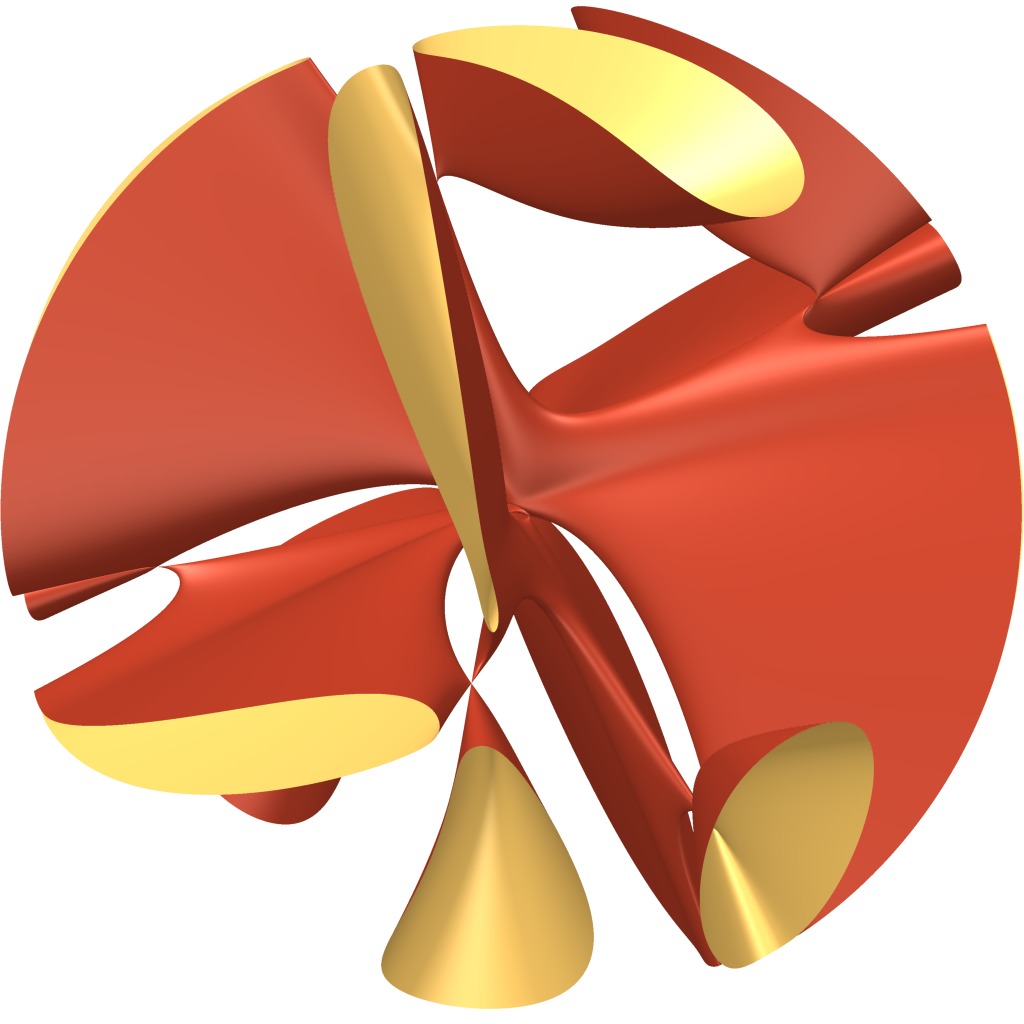
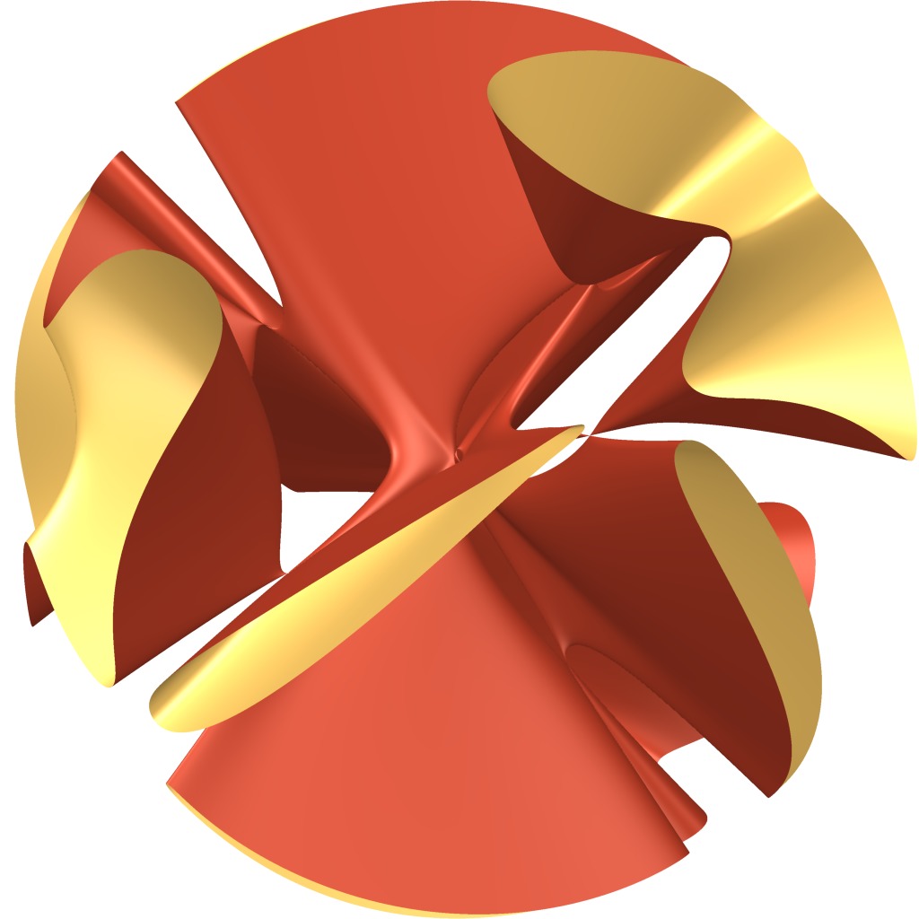
Figure 1: Part of the real locus of ${\mathscr{Z}}(g)$

2 Degree ${\boldsymbol{8k}}$

Let ${\mathscr{U}}$ denote the open subset of ${\mathbf{P}}^{3}({\mathbb{C}})$ defined by $x_{1}x_{2}x_{3}x_{4}\neq 0$ and let $\sigma_{\!k}:{\mathbf{P}}^{3}({\mathbb{C}})\rightarrow{\mathbf{P}}^{3}({\mathbb{C}})$, $[x_{1};x_{2};x_{3};x_{4}]\mapsto[x_{1}^{k};x_{2}^{k};x_{3}^{k};x_{4}^{k}]$. The restriction of $\sigma_{\!k}$ to a morphism ${\mathscr{U}}\rightarrow{\mathscr{U}}$ is an étale Galois covering, with group $({\boldsymbol{\mu}}_{k})^{4}/\Delta{\boldsymbol{\mu}}_{k}$ (here, $\Delta:{\boldsymbol{\mu}}_{k}\hookrightarrow({\boldsymbol{\mu}}_{k})^{4}$ is the diagonal embedding). We have ${\mathscr{Z}}(g[k])=\sigma_{\!k}^{-1}({\mathscr{Z}}(g))$.

Let us first prove that ${\mathscr{Z}}(g[k])$ is irreducible. We may assume that $k\hskip 1.00006pt\mathop{\geqslant}\nolimits\hskip 1.00006pt2$, as the result has been proved for $k=1$ in the previous section. Recall that

$$\frac{\partial g[k]}{\partial x_{i}}=kx_{i}^{k-1}(\frac{\partial g}{\partial x_{i}}\circ\sigma_{\!k}),$$

so the singular locus of ${\mathscr{Z}}(g[k])$ is contained in

$$\{p_{1},p_{2},p_{3},p_{4}\}\cup\Bigl{(}\bigcup_{i\neq j}\sigma_{\!k}^{-1}({\mathscr{Z}}_{i,j})\Bigr{)},$$

where $p_{i}=[\delta_{i1};\delta_{i2};\delta_{i3};\delta_{i4}]$ (and $\delta_{ij}$ is the Kronecker symbol) and ${\mathscr{Z}}_{i,j}$ is the subscheme of ${\mathbf{P}}^{3}({\mathbb{C}})$ defined by the ideal $\langle g,\frac{\partial g}{\partial x_{i}},\frac{\partial g}{\partial x_{j}}\rangle$ (and which has dimension $0$ by Lemma 3). Since $\sigma_{\!k}$ is finite, this implies that ${\mathscr{Z}}(g[k])_{\mathrm{sing}}$ has dimension $0$, so ${\mathscr{Z}}(g[k])$ is irreducible.

Now, $\sigma_{\!k}:{\mathscr{U}}\rightarrow{\mathscr{U}}$ is étale and the singular locus of ${\mathscr{Z}}(g)$ is contained in ${\mathscr{U}}$ (see Proposition 4(b)). Therefore, the $44$ singularities of ${\mathscr{Z}}(g)$ lift to $44k^{3}$ singularities in ${\mathscr{Z}}(g[k])\cap{\mathscr{U}}$ of the same type, i.e. quotient singularities of type $D_{4}$. This proves the statement (b) of Theorem 2.

Note that, for $k=2$, $3$ and $4$ (and maybe for bigger $k$) we will prove in the next sections that ${\mathscr{Z}}(g[k])$ contains singular points outside of ${\mathscr{U}}$.

3 Degree ${\boldsymbol{16}}$

Using the morphism $\sigma_{\!2}$ defined in the previous section, we get that ${\mathscr{Z}}(g[2])\cap{\mathscr{U}}$ has exactly $352$ singular points, which are all quotient singularities of type $D_{4}$. We now need to determine the singularities which are not contained in ${\mathscr{U}}$. So let ${\mathscr{H}}$ be the complement of ${\mathscr{U}}$ in ${\mathbf{P}}^{3}({\mathbb{C}})$.

> Zg2:=Surface(P3,g2);
> Zg2sing:=SingularSubscheme(Zg2);
> H:=Scheme(P3,x1*x2*x3*x4);
> Zg2singH:=Intersection(Zg2sing,H);
> time Zg2singH:=ReducedSubscheme(Zg2singH);
Time: 11.300
> irr2H:=IrreducibleComponents(Zg2singH);
> # irr2H;
18
> &+ [Degree(i) : i in irr2H];
120

The last command shows that ${\mathscr{Z}}(g)_{\mathrm{sing}}\cap{\mathscr{H}}$ contains $120$ points. We now check that all the singular points contained in ${\mathscr{H}}$ have coordinates in $L$:

> Zg2L:=ChangeRing(Zg2,L);
> sings2H:=[[Coordinates(i) :
>   i in RationalPoints(ChangeRing(j,L))] :
>   j in irr2H];
> sings2H:=&cat sings2H;
> sings2H:=[Zg2L ! i : i in sings2H];
> # sings2H;
120

We now determine the $W_{2}$-orbits in ${\mathscr{Z}}(g)_{\mathrm{sing}}\cap{\mathscr{H}}$: there is one $W_{2}$-orbit of cardinality $24$ (and we check that its elements are quotient singularities of type $A_{1}$) and one of cardinality $96$.

> orbits2:=[];
> test:=sings2H;
> W2L:=ChangeRing(W2,L);
> while (# test) gt 0 do
while>   orb:=ProjectiveOrbit(W2L,test[1]);
while>   orb:=[Zg2L ! Coordinates(i) : i in orb];
while>   orbits2:=orbits2 cat [orb];
while>   test:=[i : i in test | (i in orb) eq false];
while> end while;
> [# i : i in orbits2];
[ 24, 96 ]
> IsSimpleSurfaceSingularity(orbits2[1][1]);
true A 1

We now study the singularity of ${\mathscr{Z}}(g[2])$ at the points of the orbit of cardinality $96$. It turns out that that the command IsSimpleSurfaceSingularity takes too much time to get a conclusion, so we will investigate properties of the equation of ${\mathscr{Z}}(g[2])$ in a neighborhood of the first point $p$ (in Magma list orbits[2]). We work in the affine chart $x_{3}\neq 0$ (where $p=[\xi_{1};\xi_{2};\xi_{3};\xi_{4}]$ lives), and we denote by $(x,y,z)$ the coordinates of the affine chart $x_{3}\neq 0$ equal to $(x_{1}/x_{3}+\xi_{1}/\xi_{3},x_{2}/x_{3}+\xi_{2}/\xi_{3},x_{4}/x_{3}+\xi_{4}/\xi_{3})$ and we set

$$f(x,y,z)=g[2](x,y,1,z).$$

If $j\hskip 1.00006pt\mathop{\geqslant}\nolimits\hskip 1.00006pt0$, we denote by $f_{j}$ the homogeneous component of $f$ of degree $j$. As $p\in{\mathscr{Z}}(g[2])_{\mathrm{sing}}$, we have $f_{0}=f_{1}=0$.

> p:=orbits2[2][1];
> A3L<x,y,z>:=AffineSpace(L,3);
> cop:=Coordinates(p);
> f:=Evaluate(g2L,[x+cop[1],y+cop[2],1,z+cop[4]]);
> cof:=Coefficients(f);
> mof:=Monomials(f);
> l:=# mof;
> f2:=&+ [cof[i]*mof[i] : i in [1..l] |
>   Degree(mof[i]) eq 2];
> Factorization(f2);
[
    <y^2 + 1/4550725*(-298386*xi^7 + 4375808*xi^6
    - 795576*xi^5 + 3978000*xi^4 - 99422*xi^3
    - 1989000*xi^2 + 696114*xi - 3679654)*alpha*y*z
    + 1/182029*(201619*xi^6 - 403238*xi^2 - 472435)*z^2, 1>
]

The last command shows that there exists a linear change of the coordinates $(x,y,z)\mapsto(x,Y,Z)$ such that $f_{2}$ might be transformed into $Y^{2}+Z^{2}$. By standard arguments, this proves that $p$ is a quotient singularity of type $A_{k}$, for some $k\hskip 1.00006pt\mathop{\geqslant}\nolimits\hskip 1.00006pt2$, which can be obtained as the Milnor number of $f$: however, Magma cannot compute this Milnor number in a reasonable amount of time and we need to copy the polynomial $f$ in the software Singular [DGPS] to compute this Milnor number (!): we obtain $2$. So $p$ is a quotient singularity of type $A_{2}$. This completes the proof of statement (c) of Theorem 2.

Figure 2 shows part of the real locus of ${\mathscr{Z}}(g)$.

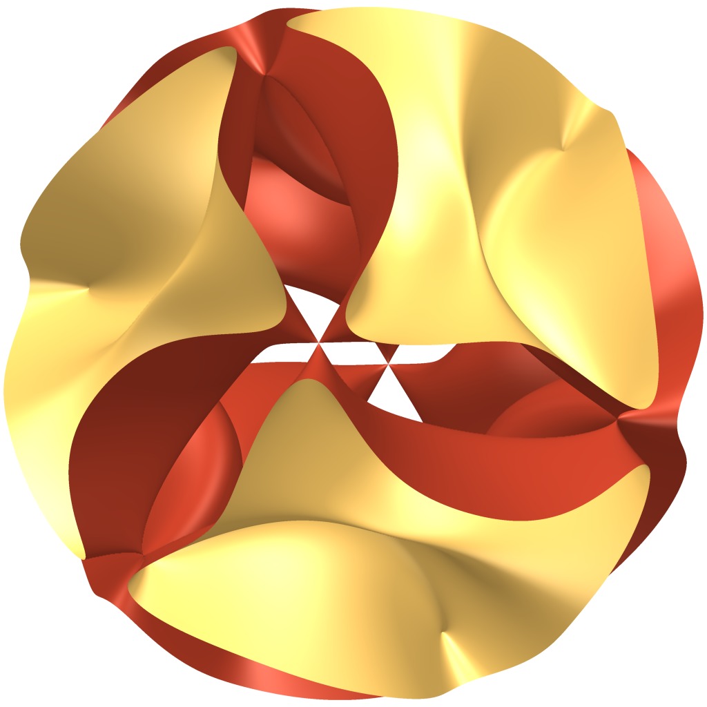
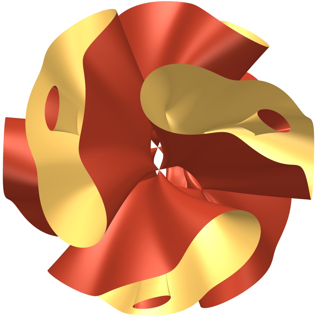
Figure 2: Part of the real locus of ${\mathscr{Z}}(g[2])$

4 Degree ${\boldsymbol{24}}$

Using the morphism $\sigma_{\!3}$ defined in Section 2, we get that ${\mathscr{Z}}(g[3])\cap{\mathscr{U}}$ has exactly $44\times 3^{3}=1~{}\!188$ singular points, which are all quotient singularities of type $D_{4}$. Let us compute ${\mathscr{Z}}(g[3])_{\mathrm{sing}}\cap{\mathscr{H}}$:

> Zg3:=Surface(P3,g3);
> Zg3sing:=SingularSubscheme(Zg3);
> Zg3singH:=Intersection(Zg3sing,H);
> time Zg3singH:=ReducedSubscheme(Zg3singH);
Time: 19.320
> time irr3H:=IrreducibleComponents(Zg3singH);
Time: 18.170
> # irr3H;
72
> Set([Degree(i) : i in irr3H]);
{ 2, 4 }
> &+ [Degree(i) : i in irr3H];
252

The last command shows that ${\mathscr{Z}}(g[3])_{\mathrm{sing}}\cap{\mathscr{H}}$ contains $252$ points. We now show that they are all defined over $K$:

> Zg3K:=ChangeRing(Zg3,K);
> sings3H:=[[Coordinates(i) :
>   i in RationalPoints(ChangeRing(j,K))] :
>   j in irr3H];
> sings3H:=&cat sings3H;
> sings3H:=[Zg3K ! i : i in sings3H];
> # sings3H;
252

So ${\mathscr{Z}}(g[3])_{\mathrm{sing}}$ contains $1440$ points, and we now check that $W_{3}$ acts transitively on them:

> p:=sings3H[1];
> time # ProjectiveOrbit(W3,p);
1440
Time: 29.850

The proof of statement (d) of Theorem 2 is complete: Figure 3 gives partial views of its real locus.

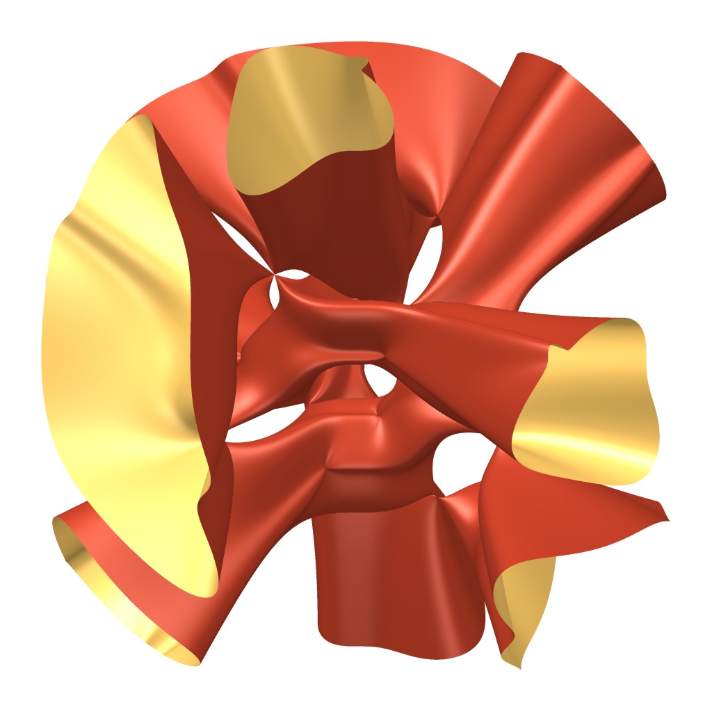
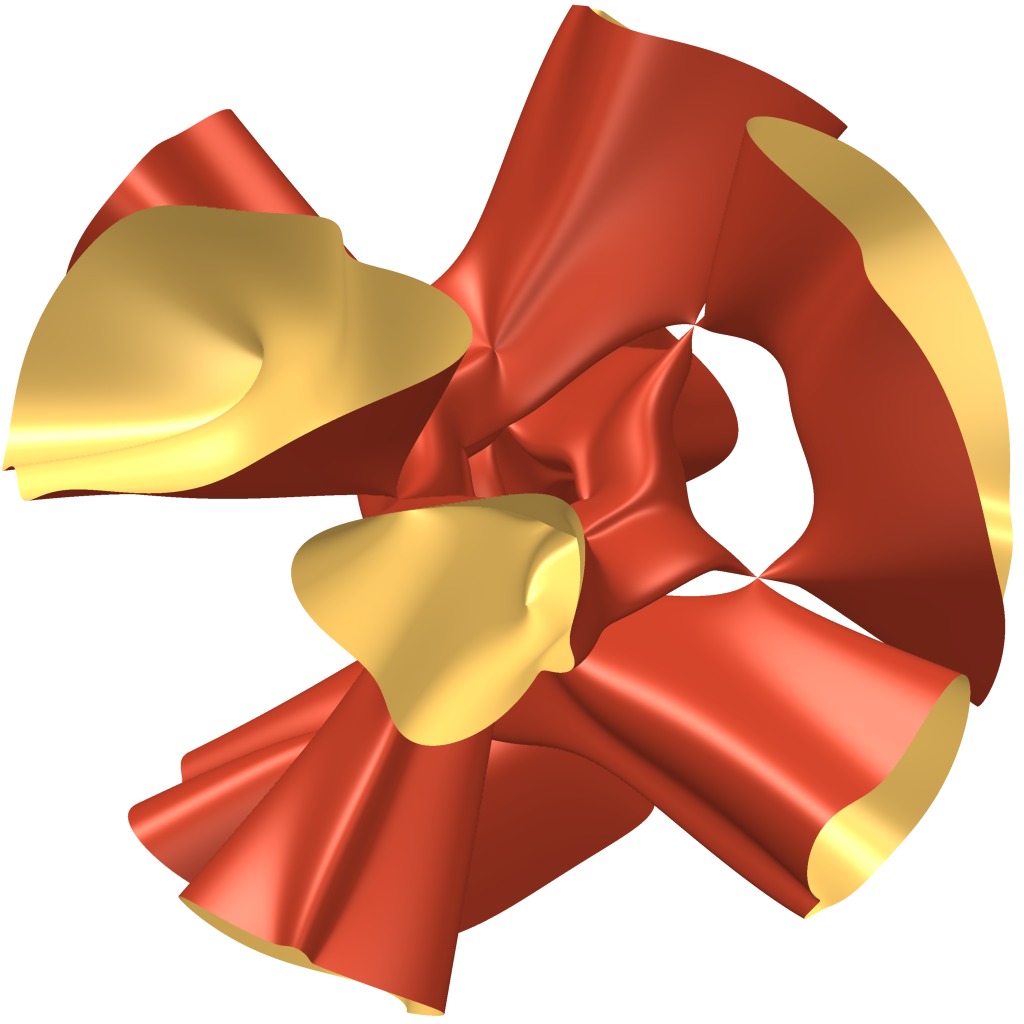
Figure 3: Part of the real locus of ${\mathscr{Z}}(g[3])$

5 Complements

Remark 3. From Section 2, we deduce that ${\mathscr{Z}}(g[4])_{\mathrm{sing}}$ has $2~{}\!816$ quotient singularities of type $D_{4}$ lying in the open subset ${\mathscr{U}}$ and it can be checked that it has $480$ other singular points not lying in ${\mathscr{U}}$, for which we did not determine the type. $\blacksquare$

Remark 4. After investigations in the invariant rings of several irreducible primitive complex reflection groups (there are $34$ such groups, denoted by $G_{i}$ with $4\hskip 1.00006pt\mathop{\leqslant}\nolimits\hskip 1.00006pti\hskip 1.00006pt\mathop{\leqslant}\nolimits\hskip 1.00006pt37$ in Shephard–Todd classification [ShTo]), we have also been able to construct curves with many singularities. For example:

• Using the reflection group $W=G_{24}$, we have obtained a cuspidal curve ${\mathscr{C}}_{14}$ of degree $14$ in ${\mathbf{P}}^{2}({\mathbb{C}})$ with exactly $42$ cusps (all lying in a single $W$-orbit). Note that $W/{\mathrm{Z}}(W)\subset\operatorname{{\mathrm{Aut}}}({\mathscr{C}}_{14})$ has order $168$ and is isomorphic to ${\mathbf{G}}{\mathbf{L}}_{3}({\mathbb{F}}_{\!2})$.

• Using the reflection group $W=G_{26}$, we have obtained a curve ${\mathscr{C}}_{18}$ of degree $18$ in ${\mathbf{P}}^{2}({\mathbb{C}})$ with $72$ cusps and $12$ nodes (these are the two $W$-orbits of singular points). Note that $W/{\mathrm{Z}}(W)\subset\operatorname{{\mathrm{Aut}}}({\mathscr{C}}_{18})$ has order $216$.

Also, other singular surfaces have been obtained. For example:

• Using the reflection group $W=G_{29}$ (note that $W/{\mathrm{Z}}(W)$ has order $1~{}\!920$), we have obtained:

  • a surface of degree $8$ in ${\mathbf{P}}^{3}({\mathbb{C}})$ with $160$ nodes, all belonging to the same $W$-orbit. Recall that the Endraß octic [End] has degree $8$ and $168$ nodes (and its automorphism group has order $16$) and the Sarti octic [Sar1] has $144$ nodes.

  • a surface of degree $8$ in ${\mathbf{P}}^{3}({\mathbb{C}})$ with $20$ singular points of multiplicity $3$ and Milnor number $11$, all belonging to the same $W$-orbit.

• Using the reflection group $W=G_{31}$, we have obtained a surface ${\mathscr{S}}_{20}$ of degree $20$ in ${\mathbf{P}}^{3}({\mathbb{C}})$ with $1~{}\!920$ nodes, all lying in the same $W$-orbit. Note that $W/{\mathrm{Z}}(W)\subset\operatorname{{\mathrm{Aut}}}({\mathscr{S}}_{20})$ has order $11~{}\!520$) and recall that the Chmutov surface [Chm] of degree $20$ has $2~{}\!926$ nodes.

Details will appear in a forthcoming paper [Bon]. $\blacksquare$

Acknowledgements. This paper is based upon work supported by the National Science Foundation under Grant No. DMS-1440140 while the author was in residence at the Mathematical Sciences Research Institute in Berkeley, California, during the Spring 2018 semester. The hidden computations which led to the discovery of the polynomial $g$ were done using the High Performance Computing facilities of the MSRI.

I wish to thank warmly Alessandra Sarti, Oliver Labs and Duco van Straten for useful comments and references and Gunter Malle for a careful reading of a first version of this note. Figures were realized using the software SURFER [Sur].

Appendix

This appendix gives a copy of the file g32-article.m loaded at the beginning of the computations. It contains the data of the polynomial $g$, the fields $K$ and $L$, the three groups $W_{i}$ and the function ProjectiveOrbit which is used throughout the computations (it is certainly not the most efficient code, but it is sufficient for our purpose). Note that $W_{1}$ and $W_{3}$ are defined over the field $K$, while $W_{2}$ is defined over the field $L$.

Q:=RationalField();
P3<x1,x2,x3,x4>:=ProjectiveSpace(Q,3);
K<zeta>:=CyclotomicField(12);
zeta3:=zeta^4;
P3K:=ProjectiveSpace(K,3);
K24<xi>:=CyclotomicField(24);
zeta4:=xi^6;
POL<T>:=PolynomialRing(K24);
L<alpha>:=NumberField(T^2-(18*xi^6 + 14*xi^5
  + 48*xi^4 + 2*xi^3 - 36*xi^2 - 14*xi - 24));
P3L:=ProjectiveSpace(L,3);

g:=x1^8 + x2^8 + x3^8 + x4^8
- 6*(x1^6*x2^2 + x1^6*x3^2 + x1^6*x4^2 + x1^2*x2^6
   + x2^6*x3^2 + x2^6*x4^2 + x1^2*x3^6 + x2^2*x3^6
   + x3^6*x4^2 + x1^2*x4^6 + x2^2*x4^6 + x3^2*x4^6)
- 60*(x1^6*x2*x3 + x1^6*x2*x4 - x1^6*x3*x4
    + x1*x2^6*x3 - x1*x2^6*x4 + x2^6*x3*x4
    + x1*x2*x3^6 + x1*x3^6*x4 - x2*x3^6*x4
    - x1*x2*x4^6 - x1*x3*x4^6 - x2*x3*x4^6)
+ 2240*(x1^5*x2^2*x3 - x1^5*x2^2*x4 + x1^5*x2*x3^2
      - x1^5*x2*x4^2 + x1^5*x3^2*x4 - x1^5*x3*x4^2
      + x1^2*x2^5*x3 + x1^2*x2^5*x4 + x1*x2^5*x3^2
      + x1^2*x2*x3^5 - x1*x2^5*x4^2 + x2^2*x3*x4^5
      - x2*x3^5*x4^2 + x2^2*x3^5*x4 + x1^2*x2*x4^5
      - x2*x3^2*x4^5 - x1*x2^2*x4^5 - x1^2*x3*x4^5
      - x1^2*x3^5*x4 + x1*x2^2*x3^5 - x1*x3^5*x4^2
      + x1*x3^2*x4^5 - x2^5*x3^2*x4 - x2^5*x3*x4^2)
- 14*(x1^4*x2^4 + x1^4*x3^4 + x1^4*x4^4
    + x2^4*x3^4 + x2^4*x4^4 + x3^4*x4^4)
+ 10180*(x1^4*x2^3*x3 + x1^4*x2^3*x4 + x1^4*x2*x3^3
       + x1^4*x2*x4^3 - x1^4*x3^3*x4 - x1^4*x3*x4^3
       + x1^3*x2^4*x3 - x1^3*x2^4*x4 + x1^3*x2*x3^4
       - x1^3*x2*x4^4 + x1^3*x3^4*x4 + x1*x2^4*x3^3
       + x1*x3^4*x4^3 - x1*x3^3*x4^4 + x2^4*x3*x4^3
       - x2^3*x3^4*x4 - x1*x2^4*x4^3 + x1*x2^3*x3^4
       - x1*x2^3*x4^4 - x2^3*x3*x4^4 - x2*x3^4*x4^3
       - x2*x3^3*x4^4 + x2^4*x3^3*x4 - x1^3*x3*x4^4 )
+ 40412*(x1^4*x2^2*x3^2 + x1^4*x2^2*x4^2 + x1^4*x3^2*x4^2
       + x1^2*x2^4*x3^2 + x1^2*x2^4*x4^2 + x1^2*x3^4*x4^2
       + x1^2*x3^2*x4^4 + x1^2*x2^2*x3^4 + x1^2*x2^2*x4^4
       + x2^4*x3^2*x4^2 + x2^2*x3^4*x4^2 + x2^2*x3^2*x4^4)
- 23440*(x1^4*x2^2*x3*x4 - x1^4*x2*x3^2*x4
       - x1^4*x2*x3*x4^2 + x1^2*x2*x3^4*x4
       + x1^2*x2*x3*x4^4 - x1^2*x2^4*x3*x4
       - x1*x2^4*x3*x4^2 - x1*x2^2*x3^4*x4
       + x1*x2^2*x3*x4^4 - x1*x2*x3^4*x4^2
       + x1*x2*x3^2*x4^4 + x1*x2^4*x3^2*x4 )
+ 111980*(x1^3*x2^3*x3^2 - x1^3*x2^3*x4^2 + x1^3*x2^2*x3^3
        - x1^3*x2^2*x4^3 - x1^3*x3^3*x4^2 + x1^3*x3^2*x4^3
        + x1^2*x2^3*x3^3 + x1^2*x2^3*x4^3 - x1^2*x3^3*x4^3
        - x2^3*x3^3*x4^2 - x2^3*x3^2*x4^3 + x2^2*x3^3*x4^3)
+ 154704*x1^2*x2^2*x3^2*x4^2;
g2:=Evaluate(g,[x1^2,x2^2,x3^2,x4^2]);
g3:=Evaluate(g,[x1^3,x2^3,x3^3,x4^3]);

s1:=Matrix(K,4,4,
[[ 0,  1,  0,  0],
 [ 1,  0,  0,  0],
 [ 0,  0,  1,  0],
 [ 0,  0,  0, -1]]);
s2:=Matrix(K,4,4,
[[ 1,  0,  0,  0],
 [ 0,  0,  1,  0],
 [ 0,  1,  0,  0],
 [ 0,  0,  0, -1]]);
s3:=Matrix(K,4,4,
[[-1,  0,  0,  0],
 [ 0,  1,  0,  0],
 [ 0,  0,  0,  1],
 [ 0,  0,  1,  0]]);
W1:=MatrixGroup<4,K | [s1,s2,s3]>;

t1:=Matrix(L,4,4,
[[ 0,  1,  0,     0],
 [ 1,  0,  0,     0],
 [ 0,  0,  1,     0],
 [ 0,  0,  0, zeta4]]);
t2:=Matrix(L,4,4,
[[ 1,  0,  0,     0],
 [ 0,  0,  1,     0],
 [ 0,  1,  0,     0],
 [ 0,  0,  0, zeta4]]);
t3:=Matrix(L,4,4,
[[-zeta4, 0,  0,  0],
 [     0,  1,  0,  0],
 [     0,  0,  0,  1],
 [     0,  0,  1,  0]]);
W2:=MatrixGroup<4,L | [t1,t2,t3]>;

u1:=Matrix(K,4,4,
[ [     1,     0,     0,     0 ],
  [     0,     1,     0,     0 ],
  [     0,     0, zeta3,     0 ],
  [     0,     0,     0,     1 ]]);
u2:=Matrix(K,4,4,
[ [(zeta3+2)/3, (zeta3-1)/3, (zeta3-1)/3, 0 ],
  [(zeta3-1)/3, (zeta3+2)/3, (zeta3-1)/3, 0 ],
  [(zeta3-1)/3, (zeta3-1)/3, (zeta3+2)/3, 0 ],
  [          0,           0,           0, 1 ]]);
u3:=Matrix(K,4,4,
[ [     1,     0,     0,     0 ],
  [     0, zeta3,     0,     0 ],
  [     0,     0,     1,     0 ],
  [     0,     0,     0,     1 ]]);
u4:=Matrix(K,4,4,
[ [(zeta3+2)/3,(1-zeta3)/3, 0,(1-zeta3)/3 ],
  [(1-zeta3)/3,(zeta3+2)/3, 0,(zeta3-1)/3 ],
  [          0,          0, 1,          0 ],
  [(1-zeta3)/3,(zeta3-1)/3, 0,(zeta3+2)/3 ]]);
W3:=MatrixGroup<4,K | [u1,u2,u3,u4]>;

// ProjectiveOrbit computes orbit of
// points in projective space

ProjectiveOrbit:=function(grp,pt)
    local i,j,res,v,w,V,PROJ,grpmod,zgrp;
  zgrp:=Centre(grp);
  zgr:=[w : w in zgrp | IsScalar(w)];
  zgrp:=sub<grp | zgrp>;
  grpmod:=Transversal(grp,zgrp);
  V:=VectorSpace(grp);
  PROJ:=AmbientSpace(Scheme(pt));
  v:=V ! Coordinates(pt);
  res:=[PROJ ! Coordinates(V,v*Transpose(w)) : w in grp];
  return [i : i in Set(res)];
end function;