BrainSlug: Transparent Acceleration of Deep Learning Through Depth-First Parallelism

Abstract

Neural network frameworks such as PyTorch and TensorFlow are the workhorses of numerous machine learning applications ranging from object recognition to machine translation. While these frameworks are versatile and straightforward to use, the training of and inference in deep neural networks is resource (energy, compute, and memory) intensive.

In contrast to recent works focusing on algorithmic enhancements, we introduce BrainSlug, a framework that transparently accelerates neural network workloads by changing the default layer-by-layer processing to a depth-first approach, reducing the amount of data required by the computations and thus improving the performance of the available hardware caches. BrainSlug achieves performance improvements of up to 41.1% on CPUs and 35.7% on GPUs. These optimizations come at zero cost to the user as they do not require hardware changes and only need tiny adjustments to the software.

1 Introduction

Artificial intelligence, and neural networks in particular, have gained immense notoriety in the past few years. Their flexibility means that they can be applied to a wide range of applications, from recommendation systems for online stores, to autonomous driving, to financial fraud detection or optimization of production lines.

One of the main issues with neural networks is their high computational time. While over the years many algorithmic and hardware optimizations to reduce the cost of these computations have arisen, the sequential way in which a neural network is processed, taking input data and computing on it from layer to layer before moving onto the next input data, has remained largely fixed. Even though this breadth-first processing is straightforward, the fact that each pass through the network acts on a relatively large amount of data causes constant cache trashing (whether on CPUs, GPUs, or other hardware), reducing their effectiveness and ultimately increasing computation time. This partly explains why processors with extremely high memory throughput are used for neural networks so that the processors are never idle.

In this report we propose the use of a depth-first approach: we take a subset of the input data (e.g., a part of an image) that can fit in L1 cache and compute all layers, then repeat the process for the next subset of the data. At this high level the process sounds simple; however, there are two main issues. First, only certain operations (i.e., layer types) are able to function when given only a subset of the data. Second, processing data in this way requires the user to write specialized compute kernels for each possible sequence of layers. This is clearly difficult to do by hand and points to the need of an automated system to carry this out.

We implemented BrainSlug (brainslug.info), a system that enables depth-first computation of neural networks, providing transparent acceleration through improvements to data locality. We make the following specific contributions:

• A novel, depth-first method for neural network computation that increases data locality and reduces computation time. The method does not change the actual results of the computation, and is widely applicable to a large set of neural networks and different types of hardware.

• An implementation of this method, including a modular architecture that allows for easy extensibility to multiple neural network frameworks (e.g., PyTorch [24], Theano [32], Caffe [3], TensorFlow [7]) and hardware targets (e.g., CPUs, GPUs, FPGAs, etc.).

• The implementation and evaluation of BrainSlug using a PyTorch front-end and CPU and GPU back-ends. Through extensive experimentation we show that BrainSlug achieves speed-ups of up to 41.1% on CPUs and 35.7% on GPUs while requiring only tiny adjustments to a user’s program.

In the following, we first give a brief background about neural networks in Section 2. Section 3 describes the main idea behind BrainSlug, followed in Section 4 by a description of the system’s implementation, and an in-depth evaluation in Section 5. Finally, we discuss related work in Section 6 and conclude in Section 7 with a discussion and future work.

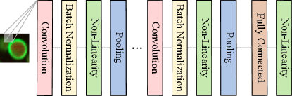
Figure 1: Typical instance of a deep convolutional neural network. All CNNs have convolutional and non-linearity layers. While the normalization and pooling layers are optional, they are found in almost all of the existing CNNs for computer vision tasks.

2 Background on Neural Networks

On a basic level, a neural network corresponds to a sequence of operations which act on numerical input data of a certain predefined size, so-called tensors. In computer vision, for instance, the input tensors are typically three-dimensional data structures, with two dimensions defining the two-dimensional picture (of $w\times h$ pixels), and the third dimension $d$ containing the information of each color channel. The naming of those three dimensions as width, height, and channels has been adopted as a common general naming scheme beyond the field of computer vision.

The transformations applied to the input data are grouped into layers, with each layer executing a certain type of operation (an example of a deep neural network is given in Figure 1). The most common layers are:
(1) Element-wise layers apply a function to each of the input tensor’s values independently. Typical examples of element-wise layers are normalization and non-linearity layers. The former normalize the output of a previous layer to conform to a specific desired distribution, improving convergence behavior and accuracy of the network. A non-linear or activation layer applies an activation function element-wise to the input. A commonly used activation function is the rectified linear unit (ReLU), computing $f(x)=\max(0,x)$ on each input [20].
(2) Pooling layers operate on predefined and fixed regions of the input tensor. These predefined regions are often non-overlapping and square-shaped. An example of two pooling operations (average and maximum) is given in Figure 2.
(3) Convolutional layers apply a convolution operation. In the image example, a convolutional layer comprises $k$ groups of $d$ filters each, where in each group one of the filters gets applied to each channel. Since each filter works on a 2-D channel, each of the $k$ groups is also called a 3-D filter (Figure 3). The output dimension of a convolutional layer has depth $k$, while keeping the channel dimensions $w\times h$.
(4) Fully-connected or dense layers: Each value of the output vector is a weighted sum of all input values, that is, all output values are connected to all input values. In deep CNNs, there are usually only a few dense layers and these are located at the end of the network (see Figure 1).

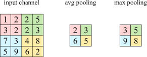
Figure 2: Example of a pooling operation on one input channel. The aggregation is performed over non-overlapping regions of the input space. The figure is based on an example from the Caffe tutorial [15].

Each neural network can be mapped to a Directed Acyclic Graph (DAG) whose nodes correspond to (groups of) element-wise operations and whose edges represent the input-output relationships between the computations. Most deep learning frameworks map a given neural network specification to such a computation graph and execute the graph on one or multiple devices. Since the DAG has a unique root (corresponding to the input data), every node has a unique depth. A level of a computation DAG is made up of all operations at a specific depth. All nodes at the same level compute their operations independently of each other, but nodes at deeper levels might depend on results of nodes in previous levels. The computation DAG, therefore, also represents the dependency structure of the computations. Figure 5 illustrates the connection between the layers of a neural network (right), the computation graph (left), and the corresponding code snippet (center).

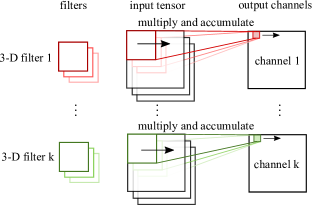
Figure 3: Each convolutional layer moves a set of 2-D filters (each being part of one 3-D filter) over the input channels from left to right and top to bottom and multiplies and accumulates the corresponding values.

⬇

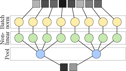
foreach x in input:

a = batchNorm(x)

foreach x in a:

b = max(x, 0)

output[0] = max(b[:4])

output[1] = max(b[4:])

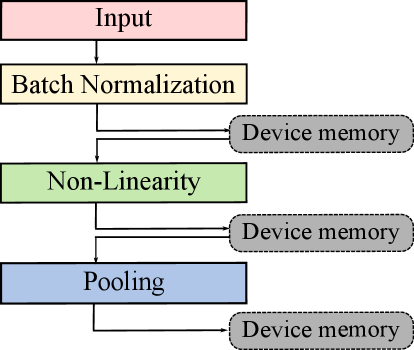
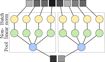
Figure 4: Breadth-first parallelism. The computation graph (left) for the neural network layers (right) and the corresponding code snippet (middle). The standard method for processing the layers is in a breath-first manner, with every operation of level $i$ in the computation graph executed in parallel before operations at level $i+1$. This is indicated by the white boxes (left) surrounding each level of the computation graph.

⬇

foreach x in input[:4]:

a[x] = batchNorm(x)

b[x] = max(a[x], 0)

output[0] = max(b)

foreach x in input[4:]:

a[x] = batchNorm(x)

b[x] = max(a[x], 0)

output[1] = max(b)

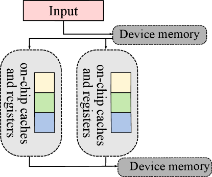
Figure 5: Depth-first parallelism. The computation graph (left) for the neural network layers (right) and the corresponding code snippet (middle). BrainSlug can detect independent paths in the computation graphs and aggregate these paths into independent processing blocks. The white boxes (left) indicate the parts of the computation graph that BrainSlug chose to parallelize. The intermediate data generated within these blocks fits into the hardware cache.

3 BrainSlug: Method Principles

Every DNN has to perform numerous passes through the network during training and prediction. In many cases, millions of floating-point operations are required for one pass and there are millions of passes per training task. With BrainSlug we want to improve the resource utilization of DNN frameworks, with a focus on accelerating (groups of) element-wise and pooling layers, all the while ensuring that this acceleration is transparent to users and that it can be implemented irrespective of the deep learning framework used (e.g., PyTorch, Theano, Caffe) and irrespective of the target hardware.

Towards this goal, we address the shortcoming of existing deep learning frameworks that always execute neural networks layer by layer. The dependency structure of the computation graph, however, allows us to exploit situations in which a different execution pattern is possible. Our work on BrainSlug is therefore motivated by two basic questions:

1. Are there ways to rearrange the standard execution order of the computation graph such that the hardware can operate more efficiently while delivering the same numerical results?

2. Is there a method for detecting when such a rearranging is possible such that it is both frequently applicable and efficient to compute?

With the proposed BrainSlug approach, we answer both questions in the affirmative. First, we show that the way in which the computation graph is executed has an impact on the efficiency of the computations. In several situations, the same set of operations can be executed such that the intermediate data fits into the caches and registers of a device, circumventing the need to read and write from the device’s main memory. This is possible by executing independent paths (or groups of independent paths) in the computation graph in parallel, essentially parallelizing the computation graph not only in a breadth-first but, when beneficial, in a depth-first manner. Second, we show that for a large class of DNNs, there is a generic method for detecting independent paths whose intermediate data fits into the caches and registers.

⬇

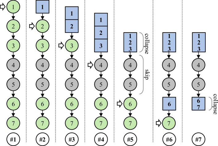
1stack = []

2foreach(node in network):

3 if(node is optimizable):

4 if(stack is empty):

5 network.replace(node, stack)

6 else

7 network.remove(node)

8 stack.add(node)

9 else:

10 stack.collapse()

11 stack = []

Figure 6: BrainSlug’s layer aggregation process, shown visually (left) and as pseudo-code (right).

3.1 Depth-First Parallelism

Existing deep learning frameworks parallelize the computation graph in a breadth-first manner, finishing all computations at one level of computation before starting the next level’s computations. We refer to this as breadth-first parallelism because the operations at one DAG level are executed in parallel before the computation proceeds to lower DAG levels.

BrainSlug is able to detect and execute more complex independent computation paths in parallel. While this does not reduce the overall number of operations, it often leads to situations where the data accessed by these independent paths fit into the caches and registers of the hardware, increasing performance. We refer to the parallel processing of independent paths in the computation graph as depth-first parallelism. The challenge is now to transparently detect and interleave these parallelism types to suit the characteristics of particular hardware.

Figure 5 illustrates depth-first parallelism for the example in Figure 5. The computation graph is the same but the operations are grouped according to the independent computation paths involving the normalization and non-linear operations, which are merged in the pooling layer. Whereas in the typical breath-first, layer-wise execution of DNNs the data has to be written and read from main memory for each layer, here the intermediate data are small enough to fit into the hardware’s cache, improving overall performance. Fortunately, as we show in what follows, detecting the existence of these parallel computation paths in the DAGs of DNNs is both efficient and frequently possible.

3.2 Aggregation Detection

To detect layers that can be aggregated, BrainSlug parses through the DAG of a given neural network layer-by-layer and identifies sequences of layers that support data locality, that is, sequences of layers that operate on a sub-set of the data (e.g., a portion of an image) reducing the number of input-output dependencies in the computation graph. Examples of such layers are layers performing element-wise and pooling operations. We add all consecutive sequences of such layers to a stack (see Figure 6), which we then collapse by analyzing the underlying computations and rewriting them to utilize depth-first parallelism. A stack, therefore, partitions independent computation paths in the DAG into paralellizable code blocks such that each such block’s intermediate data fits into the device caches. As each of the SIMD units of a single device core share the same cached data, we need to find an input data region (and the corresponding combined paths in the computation DAG) that (1) is big enough to keep all SIMD units utilized during the computations and (2) does not exceed the cache size limit. As one can see in Figure 5, if one SIMD unit is mapped onto one white box, we need at least the same number of boxes as we have SIMD units to operate efficiently.

During the rewriting of the computations we need to take the dependencies of the original DAG into account. For example, as can be seen in Figure 5, the pooling layer requires all data from the element-wise layers to be calculated before it can perform its computations.

We provide a detailed description of all of BrainSlug’s mechanisms in the following sections.

4 BrainSlug: Architecture and Implementation

One of the explicit goals of BrainSlug is to transparently accelerate neural networks (NN) irrespective of the framework (e.g., PyTorch, Theano, Caffe) they are implemented in. Further, we want the acceleration to apply to a wide range of hardware devices including GPUs, CPUs, FPGAs, and vector processors, among others; this is possible because even though their architectures may vary widely, they all rely on a memory hierarchy to speed up memory accesses, precisely the hardware feature that BrainSlug targets.

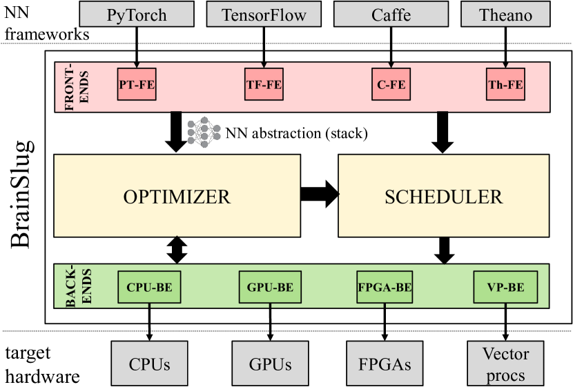
Figure 7: BrainSlug architecture consiting of front-ends (FE) that plug to existing frameworks and convert their NNs into a common abstraction; the optimizer that generates the code to transparently accelerate them; and the scheduler that executes such code, relying on the back-ends (BE) to run it on different target hardware.

To comply with these requirements, the BrainSlug architecture introduces the notion of front-ends to support different NN frameworks, and back-ends to be able to execute on different kinds of hardware (see Figure 7).

The BrainSlug front-ends are specific to a particular framework. They are in charge of parsing the NN in whatever format it is in, and providing an abstraction for it called a stack for BrainSlug’s optimizer component to use. Further, the front-ends provide glue to invoke BrainSlug’s scheduler component whenever the framework launches the prediction process.

The back-ends provide the necessary glue to have BrainSlug-generated code execute on different kinds of hardware, including providing hardware specs to the optimizer component to help it in generating the code.

Beyond these front and back-ends, BrainSlug consists of two main components: an optimizer, corresponding to a compile phase, and a scheduler, mostly in charge of the execution phase. Next, we cover each of these phases in turn, pointing out how the various components in the BrainSlug architecture interact to optimize and execute a NN. We end the section by giving a more detailed description of the PyTorch frond-end we implemented along with its API; and a discussion of the CPU and GPU back-ends.

4.1 Compile Phase

Figure 8 shows BrainSlug’s compile phase, which is primarily carried out by BrainSlug’s optimizer. The process begins when the NN framework calls the front-end’s optimize function method (Step 1 in the Figure). Next, the Network Analyzer goes through the neural network and identifies sequences of optimizable layers; a layer is optimizable if its type is in BrainSlug’s list of optimizable layers (Step 2).

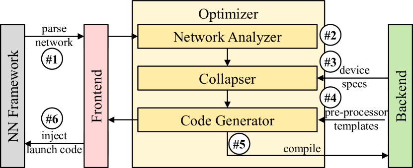
Figure 8: BrainSlug’s compile phase. The system parses a NN to identify collapsible layers (steps 1, 2), collapses those layers to fit in cache (3), inserts hardware-optimized functions into the code (4), compiles the code (5) and transparently injects the code back into the NN framework (6).

Third, the Collapser retrieves device specs from the back-end(s) (e.g., cache sizes) and takes care of reducing the layers so that their memory usage can be fit into a target cache (Step 3). In the next step (Step 5), the Code Generator retrieves device-specific pre-processor templates (Step 4) to speed up particular functions (e.g., the max function maps to fmaxf on a GPU), generates optimized code and compiles it (Step 5). Finally, the Code Generator uses the front-end to inject the code back into the NN framework (Step 6).

Collapse Process. The collapse process merits further description (see Figure 9 for a diagram and 1 for corresponding pseudo-code). To begin with, we identify optimizable layers and group them into a stack. We then map those layers onto basic computational operations: these can either be element-wise (e.g., Batch Normalization or ReLU) or non-element-wise (e.g., pooling).

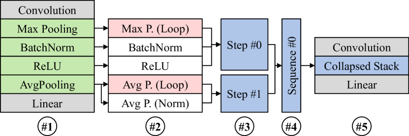
Figure 9: BrainSlug’s collapse process makes the execution of layers, and particularly the data they need, amenable to the available cache sizes. Convolution and linear layers cannot be optimized and are left untouched. Operations marked in red are non-element-wise.

Third, we assign these operations to steps. If an operation is element-wise, it can always be added to a step. If not, it can still be added to the step if there is not already another non-element-wise operation present. If this criterion is not met then we create another step: this is necessary as a non-element-wise layer’s operations depend on the output of a larger number of previous operations.

⬇

1class Stack:

2def collapse():

3 #3: group operations in steps

4 steps = []

5 step = new Step()

6 foreach(operation in optimizable):

7 if(not step.onlyElementwise() or

8 not operation.isElementwise()):

9 step.add(operation)

10 else:

11 steps.add(step)

12 step = new Step()

13

14 #4: group steps in sequences

15 sequences = []

16 sequence = new Sequence()

17 foreach(step in steps):

18 sequence.add(step)

19 if(sequence.resourceConsumption() >

20 device.resourceLimit()):

21 sequence.remove(step)

22 sequences.add(sequence)

23 sequence = new Sequence()

24

25#1: identify optimizable layers

26stack = new Stack()

27foreach(layer in graph):

28 if(isOptimizable(layer)):

29 #5: replace layers with stack

30 if(stack.empty()):

31 graph.insertBefore(layer, stack)

32 graph.remove(layer)

33

34 #2: map layer to operations

35 foreach(operation in layer);

36 stack.add(operation)

37 else:

38 stack.collapse()

Listing 1: Pseudo code explaining BrainSlug’s collapse process.

⬇

1void step_0(in_data, out_data, ...):

2 foreach(o in out_data):

3 foreach(i in in_data):

4 MaxPooling()

5 BatchNorm()

6 ReLU()

7

8void step_1(in_data, out_data, ...):

9 foreach(o in out_data):

10 foreach(i in in_data):

11 AvgPooling()

12 AvgNormalization()

13

14void sequence_0(in_data, out_data, ...):

15 float cached_data[...]

16 step_0(in_data, cached_data, ...)

17 step_1(cached_data, out_data, ...)

Listing 2: Example code of a collapsed stack.

⬇

1import torchvision.models as models

2import brainslug

3

4# load the model

5model = models.__dict__[’...’]()

6

7# optimize with BrainSlug

8brainslug.optimize(model)

9

10# execute the model

11model(...)

Listing 3: Snippet showing how to use BrainSlug’s PyTorch front-end. Only lines 2 and 8 need to be added by the user.

After this, we group the steps in order to utilize hardware resources efficiently. As each step requires that it is synchronized after it is processed, all data needs to be stored in a local data cache to pass data from one step to another. To accomplish this, we bundle these steps into sequences. We iterate over the steps and evaluate if their resource consumption fits the limitation of the target hardware (e.g., a L1 cache on a CPU or shared memory on a GPU). The resource consumption is calculated by the amount of data that each step requires and the number of active SIMD units of the processor that share this data. For example: If we have 128 SIMD units, a non-overlapping pooling layer with kernel size 3x3, and 32 channels, we would require 128*32 B for the output and 128*3*3*32 B for the input. An additional layer would have the previous input size as output, and a corresponding larger input size. If the stacked steps do not exceed the hardware resources, we add the step to the sequence, otherwise we create a new sequence.

Finally, we generate the final code. There are two possible scenarios. First, if a sequence only contains a single step, we iterate over the entire input data: in this case data locality is achieved by directly passing the values from one operation to another. If there are multiple steps, we need to perform the previously-mentioned synchronization between the steps. In the case that the cache size limit is not reached, we increase the size of it, so that each SIMD unit may not calculate a single output value, but multiple ones, to better utilize the given hardware resources. Finally, we compile the code using a device-specific compiler and replace the optimized layers in the NN with our collapsed stack. To illustrate, 2 shows how the example in Figure 9 is mapped onto the actual final code.

4.2 Execution Phase

BrainSlug’s execution phase, embodied by the scheduler, handles the execution of the compute kernels. When a stack is executed, the front-end gathers all necessary data and parameter tensors. The scheduler then calculates the output size and allocates memory using the NN framework. After this the kernel function object (cubin for GPU and dll for CPU) is loaded, executed and the result buffer is returned to the NN framework. If there is more than one sequence in a stack the sequences are executed in a serialized fashion.

4.3 PyTorch Front-end and API

We implemented a PyTorch front-end. We chose PyTorch as it was the first NN framework to support dynamic network graphs that can be reshaped at runtime. This feature complicates the implementation but allows us to show that our method can be applied even in such a highly dynamic scenario.

The frontend parses through the neural network, groups all optimizable layers in stacks and passes these to the BrainSlug optimizer. These are then removed from the network and replaced by a special BrainSlug layer (one per stack) that pass the control flow to the BrainSlug scheduler whenever they are triggered. If there are multiple equivalent stacks, BrainSlug only generates the code once and reuses it for all identical stacks.

Finally, it is worth noting that the front-end is extremely easy to use: the user need only add a few lines of code in order to enable transparent acceleration of the neural networks (see 3).

4.4 CPU and GPU Backends

GPU: GPUs are often used for processing of neural networks, mainly because of their high compute performance and memory throughput. For the implementation we use two code building blocks.

For steps that only perform element-wise operations, we start as many thread blocks as there are channels and each thread blocks applies its calculations on each batch, for a specific channel.

For pooling layers we distinguish between stacked and non-stacked. In the non-stacked case, we start BatchSize * Channels thread blocks. The SIMD units iterate over all data elements, while we process as many element as we have SIMD units in parallel. In the stacked case, we use BatchSize * Channels * Patches thread blocks, where each patch represents a depth-first processing and use the SIMD units the same way. To store the data for the depth-first processing we use two buffers allocated in the devices shared memory. When a step is processed, we synchronize the entire thread block and swap the buffers for the next step.

In general we use a thread count of 128, which is a good trade-off between overhead when synchronizing a thread block and compute utilization. Further, we limit the usage of shared memory to 16 kB (depending on the GPU either 64 or 92 kB would be available), as this can have a negative impact on the performance because it reduces the amount of blocks that can be scheduled onto the GPU multiprocessor, resulting in less opportunities to employ latency hiding.

CPU: The CPU back-end relies on the Intel SPMD Program Compiler [13] (ISPC). ISPC can be seen as “CUDA for CPUs”: it adds syntactic sugar to the application and explicitly defines which computations should be done by a single SIMD unit. Because of the similarities between ISPC and CUDA we can share many parts of the implementation between both architectures. As CPUs do not have a dedicated shared memory, we allocate the memory on the stack. The other parts of the implementation are similar and differ only in the way variables are used – either by all or only single SIMD units – and replacing the outer loops with the ISPC specific foreach(...) instruction. ISPC can target different instruction sets, e.g. SSE[2,4], AVX[1,2] and AVX512 for Intel’s Knight’s Landing. We use the default values from the compiler. ISPC further supports a task system, similar to CUDA thread blocks. This task system has to use some predefined variants provided by ISPC or can be implemented by the user. As our task system does not require any special features, we implemented a simple variant based on parallel for using Intel’s Threading Building Blocks [14] to minimize the framework’s overhead.

5 Evaluation

To evaluate BrainSlug we chose the TorchVision[25] package. TorchVision contains a series of broadly used neural network architectures for computer vision applications. We use the entire set of available networks ranging from AlexNet (A) [16], Densenet-(121, 161, 169, and 201) (D) [9], Inception v3 (I) [31], Resnet-(18, 34, 50, 101, and 152) (R) [8], Squeezenet-(1.0 and 1.1) (S) [11], and VGG-(11, 13, 16, and 19, with and without Batch Normalization) (V) [28], a total of 21 different architecture and parameter combinations.

We run all tests on a server with an Intel Xeon E5-2690v4, an NVIDIA GeForce GTX 1080 Ti, Debian 9, NVIDIA GPU driver v384.81, CUDA v9.0, ISPC v1.9.2, Python v3.5.3 and PyTorch v0.3.0 (using cuDNN). We perform the test times ten times for the GPU and five times for the CPU and we take the minimum execution time for both PyTorch and BrainSlug results.

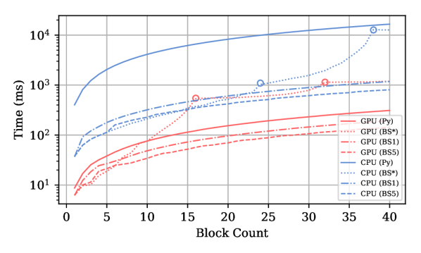
Figure 10: Performance of BrainSlug’s stacked layer mechanism versus PyTorch for increasing numbers of $<$Max-Pooling,Batch Normalization,ReLU$>$ blocks.

5.1 Stacked Layers Acceleration

For the first experiment we want to evaluate the advantage of our proposed layer stacking mechanism. To do so, we build artificial neural networks consisting only of layers that can be optimized using BrainSlug. In particular, we define a block consisting of a Max-Pooling (Kernel: 3x3, Stride: 1x1 and Padding: 1x1), a Batch Normalization and a ReLU layer, and create neural networks that comprise between 1 and 40 of these blocks. We execute these networks on a CPU and GPU (see Figure 10, notice the log scale) and evaluated three different strategies: only 1 step per sequence, max 5 steps per sequence and unrestricted.

On the CPU, the PyTorch implementation is always 10-20x slower than BrainSlug. This massive increase is partially due to the fact that the current PyTorch implementation is not particularly optimized for CPUs: most significantly, it does not use any explicit vector processing instructions. In contrast, we use ISPC for vector operations, so in theory we have 8x more computational power (AVX2 with 8x 32Bit float operations). Further, the PyTorch CPU code relies on OpenMP parallel for constructs, but does not define a specific execution schedule, yielding sub-optimal performance. On the GPU, BrainSlug yields a speed-up of 1.4-2.2x.

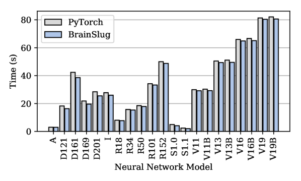
Figure 11: Comparison of calculation time between PyTorch and BrainSlug for TorchVision’s neural networks (CPU, batch size 128).

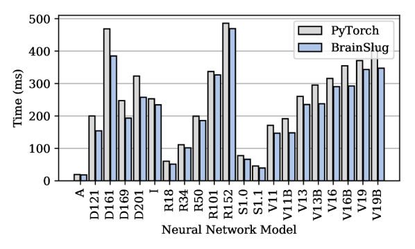
Figure 12: Comparison of calculation time between PyTorch and BrainSlug for TorchVision’s neural networks (GPU, batch size 128).

Figure 13: BrainSlug’s speed-up over PyTorch of TorchVision neural networks (CPU, batch size 128).

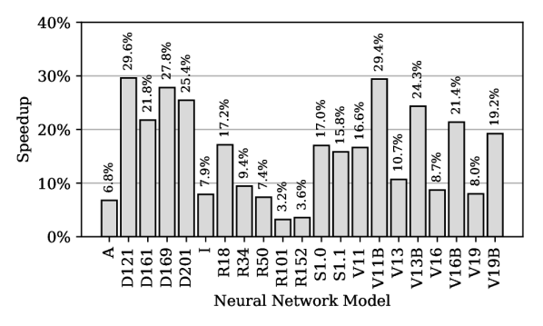
Figure 14: BrainSlug’s speed-up over PyTorch of TorchVision neural networks (GPU, batch size 128).

For both devices the performance improves even if we only allow one step per sequence. It further improves when we stack multiple steps in a sequence, up to 61% for the GPU and 58% for the CPU. In the unrestricted case, we can see that for the lower block counts it is equal or even slightly better than the 5 step scenario. However, the performance significantly decreases for larger values until it reaches an artifact (indicated by circles) that happens for the GPU at 16 and 32, and for the CPU at 24 and 38. These artifacts occur whenever the cache size limit is reached and an additional sequence is required. The cause for this increase in required cache size is the padding value of the Max-Pooling layer. This causes an overlap of data and, as previously discussed for the convolutional layers, results in redundant operations. As each block adds new padding, the value increases with each additional block. The performance improves at these points since the new sequence does not suffer from the redundant operations in the first place, but only if too many blocks are added to it.

5.2 Full Network Acceleration

Next, we evaluate the acceleration that BrainSlug provides when executing more realistic neural networks. Figures 14 and 14 show the total execution time when running the networks with a batch size of 128 for CPUs and GPUs respectively, while Figures 14 and 14 show the relative speedup with respect to PyTorch.

While the networks have significantly varying execution times ranging from very short (AlexNet) to quite long (Densenet-161 and Resnet-152), BrainSlug provides a speed up in all cases, with the most pronounced improvements for Densenets on both CPU and GPU, VGGs with Batch Normalization on GPU, and Squeezenets on CPU. Note that adding the Batch Normalization layer to the VGG networks has a significant impact on PyTorch’s computation time, while there is virtually no change in BrainSlug’s case: an effect directly attributable to BrainSlug collapsing the normalization into the previous step.

Table 1 shows BrainSlug’s full speed-up results for all networks on CPU and GPU for batch sizes from 1 to 256. The results clearly indicate that BrainSlug outperforms PyTorch on the GPU with batch sizes bigger than 8 (except for Resnet-101 and -152), and for all cases for the CPU.

⬇

1#omp parallel for

2foreach(batch):

3 #omp parallel for

4 foreach(channel):

5 ...

Listing 4: PyTorch’s Max-Pooling implementation.

The results show large performance gains for small batch sizes when running on the CPU. This is related to a programming error in PyTorch’s Max-Pooling implementation (see 4). The code uses two nested OpenMP parallel for loops, which means that only the outer loop is parallelized over the CPU cores. In the extreme case of batch size $=1$, the entire function utilizes only a single core. In BrainSlug we use only one parallel for loop, iterating over BatchSize $\times$ Channels elements, so we can always leverage parallelism.

Finally, note that negative values for the GPU batch sizes 1–-4 look significant but in absolute terms they are not: in these cases the execution time is only a few milliseconds, while for larger ones, it is hundreds of milliseconds. This relatively performance difference is mainly because our implementation is optimized towards larger batch sizes.

Table 1: BrainSlug full speed-up results compared to PyTorch on a CPU and GPU for all neural networks.

5.3 Detailed Performance Analysis

BrainSlug’s performance gains stem from optimizing some layer types, while leaving others as they are. Here we provide a more detailed analysis to answer the following question: for real-world neural networks, how much does BrainSlug improve the performance of the optimizable layers, and what fraction of the overall runtime is this optimizable part?

	Network			Opt. Speed-up [%]		% of Total Time		Total Speed-up [%]
Name	Layers	Opt.	Stacks	CPU	GPU	CPU	GPU	CPU	GPU
Alexnet	27	12	8	$483.1$	$72.7$	$3.0$	$13.7$	$2.5$	$5.8$
Inception V3	316	203	103	$451.2$	$27.5$	$8.7$	$28.6$	$7.1$	$6.2$
Densenet-121	429	247	124	$411.1$	$77.3$	$13.1$	$47.3$	$10.5$	$20.6$
Densenet-161	569	327	164	$446.9$	$68.3$	$10.9$	$38.6$	$8.9$	$15.7$
Densenet-169	597	343	172	$414.0$	$72.6$	$13.9$	$47.4$	$11.2$	$19.9$
Densenet-201	709	407	204	$415.1$	$66.5$	$13.7$	$47.1$	$11.0$	$18.8$
Resnet-18	71	39	21	$387.5$	$76.6$	$4.8$	$22.2$	$3.8$	$9.6$
Resnet-34	127	71	37	$436.4$	$60.0$	$3.6$	$17.9$	$2.9$	$6.7$
Resnet-50	177	104	54	$348.5$	$13.7$	$8.2$	$24.6$	$6.4$	$3.0$
Resnet-101	347	206	105	$321.2$	$8.2$	$6.5$	$20.7$	$5.0$	$1.6$
Resnet-152	517	308	156	$319.2$	$5.7$	$6.3$	$19.5$	$4.8$	$1.1$
Squeezenet 1.0	66	31	29	$842.9$	$34.7$	$4.5$	$29.3$	$4.0$	$7.5$
Squeezenet 1.1	66	31	29	$457.1$	$32.3$	$16.9$	$33.5$	$13.9$	$8.2$
VGG11	35	17	10	$808.3$	$113.5$	$3.8$	$21.5$	$3.3$	$11.4$
VGG11 BN	43	25	10	$842.9$	$222.9$	$4.5$	$30.2$	$4.0$	$20.9$
VGG13	39	19	12	$661.9$	$59.7$	$3.3$	$19.4$	$2.8$	$7.3$
VGG13 BN	49	29	12	$622.2$	$159.2$	$4.0$	$29.5$	$3.4$	$18.1$
VGG16	45	22	15	$665.2$	$51.7$	$2.7$	$17.2$	$2.4$	$5.9$
VGG16 BN	58	35	15	$620.0$	$146.7$	$3.4$	$26.5$	$2.9$	$15.8$
VGG19	51	25	18	$650.0$	$44.8$	$2.5$	$15.6$	$2.1$	$4.8$
VGG19 BN	67	41	18	$618.2$	$137.7$	$3.0$	$24.6$	$2.6$	$14.2$

Table 2: For each NN at batch size 128: the number of layers, how many BrainSlug can optimize and into how many stacks. Opt. Speed Up is the acceleration for the optimizable layers, % of Total Time is the time the optimized layers take within the full execution, and Total Speed Up is the speed-up for the entire network.

As shown in Table 2, the complexity of the networks ranges from 27 up to 709 layers, with BrainSlug able to optimize 44 to 64% of them using 8 to 204 stacks. For those layers, we achieve speed-ups of 321.2 to 842.9% on the CPU and 5.7 to 222.9% on the GPU (all results are for a batch size of 128). Again, the speed-up for the CPU is significantly higher than for the GPU due to PyTorch’s less-than-optimal CPU implementation. Overall, the optimizable layers represent 2.5 to 16.9% for the CPU and 13.7 to 47.4% for the GPU of the total computation time (% of Total Time columns), with the rest of the time being spent mostly on convolutional layers. This leads to a total speed-up of 2.1% to 13.9% for the CPU and 1.1% and 20.9%. Note that this speed-up only concerns the pure compute kernel time, and is hence different from the numbers for batch size 128 in Table 1; the total improvement is in fact often higher because, for example, BrainSlug needs fewer memory allocations.

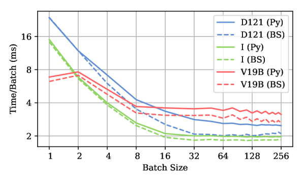
Figure 15: Scaling behavior of BrainSlug (BS) versus PyTorch (Py) for different batch sizes.

5.4 Batch Size Scaling Behavior

One important parameter for neural network performance is the batch size, which represents the number of independent data parts (e.g., images) that are processed at the same time. Most operations can operate independently on individual batches, which can be leveraged for parallelism. Figure 15 shows how PyTorch and BrainSlug scale with respect to increasing batch sizes for three selected networks. As can be seen, both scale with batch size but BrainSlug performs always best, showing increasing gains for larger batch sizes.

6 Related Work

In this work we focus on accelerating the forward pass in deep neural networks on both CPUs and GPUs. Due to the frequent occurrence of convolutional and dense layers in these networks (see Figure 1), recent work has focused specifically on improving the multiply-and-accumulate (MAC) operations prevalent in these layers. CPUs and GPUs have libraries that support SIMD or SIMT-based processing such as Intel’s “single program, multiple data” (SPMD) compilers. In general, the MAC operations resulting from convolutional and dense layers can be mapped to multiplications between two matrices. Libraries such as cuDNN [4] and cuBLAS [21] for GPUs and Intel MKL [12] and OpenBLAS [23] for CPUs are optimized for matrix–matrix operations. Moreover, there are specialized algorithms that can lead to speed-ups for the multiply operation in convolutional layers. For instance, performing a fast Fourier transform (FFT) has been shown to be beneficial for convolutional layers with certain properties [19]. There are also several other approaches that reduce the number of expensive operations required for matrix-matrix multiplications. Examples are the application of Strassen’s [5] and Winograd’s algorithms [17] for accelerating the processing of convolutional layers. Deep learning libraries such as NVIDIA’s cuDNN and TensorRT [22] utilize heuristics for choosing the algorithmic method expected to work best for a given convolutional layer. TensorRT selects different implementations according to the used hardware and optimizes memory allocation. Due to the extensive engineering that goes into the design of these heuristics and implementations, the processing of convolutional layers is highly optimized and hard to improve on; consequently, BrainSlug focuses on improvements to other commonly-used layer types.

The main disadvantage of TensorRT is that it only works if all used layers are known to the framework, as it directly translates the entire network into its own implementation for NVIDIA GPUs. BrainSlug, in contrast, only replaces parts of the network that it knows. This enables us to create and explore user-created layers and still benefit from BrainSlug’s improvements. Further, BrainSlug is designed as an extensible platform, allowing users to apply its optimizations not only to GPUs but to all kinds of processors and accelerators.

The algorithmic optimizations discussed so far do not change the network architecture or the result of the computations. There are several algorithmic tricks one can apply to trade-off accuracy for efficiency. For instance, TensorRT can reduce the precision from 32 Bit floating point to 16-Bit floating point or even 8-Bit integer, which improves performance but might decrease accuracy. It is even possible to work with binarized neural networks, that is, networks that perform binary instead of floating point operations [10, 6, 26]. There are numerous other methods that change the structure and parameters of the original DNN to improve performance. For instance, it is possible to prune filters during the learning process which reduces the amount of computation required for the convolutional layers [18]. In a different line of work, the network units with low-valued activations are pruned. This was shown to result in a 11% speed up [1] or a substantial reduction in power consumption [27]. With BrainSlug, we focus on optimizations that do not alter the original DNN: both the original and optimized DNN perform exactly the same operations on the hardware.

Alwani et al. [2] proposed to fuse layers of convolutional neural networks for faster processing on FPGAs, merging the first two convolutional layers of a neural network. Their method uses a data shifting approach to reduce the recomputation of overlapping data regions. This is quite efficient for FPGAs but is difficult to implement on CPUs and GPUs, and has the limitation of only being applicable to no more than two convolutional layers. As already mentioned, our method does not focus on convolutional layers but accelerates the entire network by aggregating consecutive non-convolutional layers.

Sze et al. [30] discuss different methods for energy-efficient dataflows on neural network accelerators, suggesting the development of a specialized neural network accelerator with a mesh-based processing architecture. In contrast, our method targets off-the-shelf, cheap hardware that provides excellent compute power per dollar.

7 Discussion and Future Work

We have shown that BrainSlug (brainslug.info) accelerates commonly used deep neural networks by as much as 41.1% on CPUs and 35.7% on GPUs while requiring minimal code changes. These improvements are significant considering that training such networks on big data can take up to several weeks. BrainSlug’s speed-up is most pronounced for the more commonly used batch sizes of 8 and up. For instance, the DenseNet architectures are usually trained with a per-GPU batch size of 32 [9], a batch size where BrainSlug achieves the best performance improvement. Due to recent results insights into the benefits of increasing the batch size during training [29] and the generally growing size of main memory on GPUs, we expect training batch sizes to further increase in the future.

Extending BrainSlug: BrainSlug is designed to make it easy to extend and, as such, provides APIs that need to be implemented when developing front and back-ends. Adding a new front-end requires the biggest effort, since it has to parse through the NN graph and identify optimizable layers; this cannot be implemented generically as every NN framework uses a different representation. Further, it is necessary to connect BrainSlug’s runtime system with the NN framework, so that BrainSlug can interact with framework-specific data structures. For PyTorch, our front-end implementation consists of 270 lines of Python code and 438 lines of C++. To add a new back-end requires much less work, as only methods to load and execute the device code are required. In our implementation, we have 299 lines of C++ code (code + header files) for NVIDIA GPUs (including integration of the NVIDIA profiling library) and 165 lines of code for CPUs.

Limitations: Although in theory our stacking method can be applied to several different kinds of layers, we figured out that in certain cases it is not beneficial. While we were able to achieve significant speed ups for element-wise and pooling layers, we have not been able to improve linear and convolutional layers. For convolutional layers the problem is that the operation itself uses overlapping data areas. Because of this overlap, BrainSlug would force neighboring data paths to have to do redundant calculations. As convolution is already a compute-bound operation, and since BrainSlug optimizes memory accesses and not the actual computation, these redundant calculations reduce overall performance. For linear layers the problem is more conceptual. A linear layer can be represented by a matrix–matrix multiplication. Instead of executing this as a matrix–matrix multiplication, BrainSlug would strip it down to multiple vector–matrix multiplications. The problem of this method is that the processor needs to load the entire weight matrix for each output vector. In contrast, in a matrix–matrix multiplication the weight matrix can be significantly better reused, resulting in less memory transactions compared to multiple vector–matrix multiplications.

Future Work: We plan to enhance BrainSlug by adding more front-ends to support a larger variety of frameworks. Further, we plan to expand our optimizations to training, as this is the most time consuming operation for neural networks; we expect BrainSlug to be able to achieve equivalent speed-ups for it. Finally, we are also targeting additional types of hardware including vector or neural network processors.

References

- [1] Albericio, J., Judd, P., Hetherington, T., Aamodt, T., Jerger, N. E., and Moshovos, A. Cnvlutin: Ineffectual-neuron-free deep neural network computing. In ACM SIGARCH Computer Architecture News (2016), vol. 44, IEEE Press, pp. 1–13.
- [2] Alwani, M., Chen, H., Ferdman, M., and Milder, P. Fused-Layer CNN Accelerators. In Proc. MICRO (2016).
-
[3]
Berkeley Artificial Intelligence Research.
Caffe.
http://caffe.berkeleyvision.org. - [4] Chetlur, S., Woolley, C., Vandermersch, P., Cohen, J., Tran, J., Catanzaro, B., and Shelhamer, E. cudnn: Efficient primitives for deep learning. arXiv preprint arXiv:1410.0759 (2014).
- [5] Cong, J., and Xiao, B. Minimizing computation in convolutional neural networks. In International conference on artificial neural networks (2014), Springer, pp. 281–290.
- [6] Courbariaux, M., Hubara, I., Soudry, D., El-Yaniv, R., and Bengio, Y. Binarized neural networks: Training deep neural networks with weights and activations constrained to+ 1 or-1. arXiv preprint arXiv:1602.02830 (2016).
-
[7]
Google Brain Team.
TensorFlow.
https://www.tensorflow.org. - [8] He, K., Zhang, X., Ren, S., and Sun, J. Deep residual learning for image recognition. In Proceedings of the IEEE conference on computer vision and pattern recognition (2016), pp. 770–778.
- [9] Huang, G., Liu, Z., Weinberger, K. Q., and van der Maaten, L. Densely connected convolutional networks. In Proceedings of the IEEE conference on computer vision and pattern recognition (2017), vol. 1, p. 3.
- [10] Hubara, I., Courbariaux, M., Soudry, D., El-Yaniv, R., and Bengio, Y. Binarized neural networks. In Advances in neural information processing systems (2016), pp. 4107–4115.
- [11] Iandola, F. N., Han, S., Moskewicz, M. W., Ashraf, K., Dally, W. J., and Keutzer, K. Squeezenet: Alexnet-level accuracy with 50x fewer parameters and 0.5mb model size. arXiv:1602.07360 (2016).
-
[12]
Intel.
Intel Math Kernel Library (Intel-MKL).
https://software.intel.com/en-us/mkl. -
[13]
Intel.
Intel SPMD Program Compiler (ISPC).
https://ispc.github.io. -
[14]
Intel.
Intel Threading Building Blocks (TBB).
https://www.threadingbuildingblocks.org. - [15] Jia, Y., Shelhamer, E., Donahue, J., Karayev, S., Long, J., Girshick, R., Guadarrama, S., and Darrell, T. Caffe: Convolutional architecture for fast feature embedding. In Proceedings of the 22nd ACM international conference on Multimedia (2014), ACM, pp. 675–678.
- [16] Krizhevsky, A., Sutskever, I., and Hinton, G. E. Imagenet classification with deep convolutional neural networks. In Proceedings of Neural Information Processing Systems (2012).
- [17] Lavin, A., and Gray, S. Fast algorithms for convolutional neural networks. In Proceedings of the IEEE Conference on Computer Vision and Pattern Recognition (2016), pp. 4013–4021.
- [18] Li, H., Kadav, A., Durdanovic, I., Samet, H., and Graf, H. P. Pruning filters for efficient convnets. arXiv preprint arXiv:1608.08710 (2016).
- [19] Mathieu, M., Henaff, M., and Lecun, Y. Fast training of convolutional networks through ffts. In International Conference on Learning Representations (ICLR) (2014).
- [20] Nair, V., and Hinton, G. E. Rectified linear units improve restricted boltzmann machines. In Proceedings of the 27th international conference on machine learning (ICML) (2010), pp. 807–814.
-
[21]
NVIDIA.
cuBLAS.
https://developer.nvidia.com/cublas. -
[22]
NVIDIA.
TensorRT.
http://developer.nvidia.com/tensorrt. -
[23]
OpenBLAS project.
OpenBLAS.
http://www.openblas.net. -
[24]
PyTorch core team.
PyTorch.
https://pytorch.org. -
[25]
PyTorch core team.
TorchVision.
https://github.com/pytorch/vision. - [26] Rastegari, M., Ordonez, V., Redmon, J., and Farhadi, A. Xnor-net: Imagenet classification using binary convolutional neural networks. In European Conference on Computer Vision (2016), Springer, pp. 525–542.
- [27] Reagen, B., Whatmough, P., Adolf, R., Rama, S., Lee, H., Lee, S. K., Hernández-Lobato, J. M., Wei, G.-Y., and Brooks, D. Minerva: Enabling low-power, highly-accurate deep neural network accelerators. In ACM SIGARCH Computer Architecture News (2016), vol. 44, IEEE Press, pp. 267–278.
- [28] Simonyan, K., and Zisserman, A. Very deep convolutional networks for large-scale image recognition. arXiv preprint arXiv:1409.1556 (2014).
- [29] Smith, S. L., Kindermans, P.-J., and Le, Q. V. Don’t decay the learning rate, increase the batch size. In International Conference on Learning Representations (ICLR) (2018).
- [30] Sze, V., Chen, Y.-H., Yang, T.-J., and Emer, J. S. Efficient processing of deep neural networks: A tutorial and survey. Proceedings of the IEEE 105, 12 (2017), 2295–2329.
- [31] Szegedy, C., Vanhoucke, V., Ioffe, S., Shlens, J., and Wojna, Z. Rethinking the inception architecture for computer vision. CoRR abs/1512.00567 (2015).
-
[32]
Universite de Montreal.
Theano.
http://deeplearning.net/software/theano/.