Spectral and Timing Properties of Atoll Source 4U 1705-44 : LAXPC/AstroSat Results

Abstract

In this paper, we present the first results of spectral and timing properties of the atoll source 4U 1705-44 using $\sim$ 100 ks data obtained with Large Area X-ray Proportional Counter (LAXPC) onboard AstroSat. The source was in the high-soft state during our observations and traced out a banana track in the Hardness Intensity Diagram (HID). We study the evolution of the Power Density Spectra (PDS) and the energy spectra along the HID. PDS show presence of a broad Lorentzian feature (Peaked Noise or PN) centered at $1-13$ Hz and a very low frequency noise (VLFN). The energy spectra can be described by sum of a thermal Comptonized component, a power-law and a broad iron line. The hard tail seen in the energy spectra is variable and contribute $4-30$% of the total flux. The iron line seen in this source is broad (FWHM $\sim$ 2 keV) and strong (EW $\sim$ $369-512$ eV). Only relativistic smearing in the accretion disc can not explain the origin of this feature and requires other mechanism such as broadening by Comptonization process in the external part of the ‘Comptonized Corona’. A subtle and systematic evolution of the spectral parameters (optical depth, electron temperature etc.) is seen as the source moves along the HID. We study the correlation between frequency of the PN and the spectral parameters. PN frequency seems to be correlated with the strength of the corona. We discuss the implication of the results in the paper.

1 Introduction

Luminous low mass X-ray binaries (LMXBs) containing weakly magnetized Neutron Stars (NSs) are divided into two groups, called Z and atoll sources, based on the pattern they trace out in the color-color diagram (CCD) and the hardness-intensity diagram (HID) (Hasinger and van der Klis, 1989). Z-sources trace out a ‘Z’ shaped path in the CCD and HID. Atoll sources trace out a C-type curve in the CCD and HID. The discovery of the transient NS LMXB XTE J1701-462 (Remillard et al., 2006) provided a connection between two subgroups of Z-sources (Sco-like and Cyg-like; see Kuulkers et al. 1994) and atoll sources. At the initial phase of the outburst (at the highest accretion rate), the source displayed behaviour like Cyg-like Z-sources and then as the source intensity decreased the source transformed into Sco-like Z-sources (Homan et al., 2007). At the lowest intensity state, the source showed behaviour like atoll sources (Lin, Remillard and Homan, 2009). The observed transitions of the source from one type to another type suggest that the accretion rate is an important regulating parameter which decides the behaviour of a NS LMXB on the CCD and HID.

The C-type track of atoll sources has two branches, island state and banana state. Luminosity and X-ray spectra of atoll sources vary as they move from the island to banana state. Luminosity of atoll sources varies between $0.001-0.5$ $L_{Edd}$ (Done et al., 2007) for a NS of mass 1.4 $M_{\odot}$. The island state is characterized by low count rates and hard energy spectra. On the other hand, in the banana state, they have higher luminosities and softer X-ray spectra (Barret, 2001). The energy spectra in both states are complex and have multiple components. Various approaches exist in literature to model the X-ray spectra of both atoll and Z-sources. X-ray spectra of these sources have two main components, one arising from the accretion disc and other from the boundary layer/surface of the NS. In one of the approaches, the spectrum is sum of the soft emission from a standard cold disk described by multi-color-disc blackbody (MCD) and a hard Comptonized component from the boundary layer (Mitsuda et al., 1984; Barret et al., 2000; Barret, 2001; Di Salvo et al., 2002; Agrawal and Sreekumar, 2003; Tarana, Bazzano, Ubertini, 2008; Agrawal and Misra, 2009). In an another approach, the hot inner disc radiates a hard Comptonized component and the boundary layer radiates a soft single temperature blackbody (BB) (Di Salvo et al., 2000, 2001; Sleator et al., 2016). Sometime two thermal components, one from the accretion disc (MCD) and another from a boundary layer (BB) are also used (Lin, Remillard and Homan, 2007, 2010) to model the energy spectrum.

The source 4U 1705-44 is a type-I X-ray burster (Gottwald and Haberl, 1989) and is classified as an atoll source (Hasinger and van der Klis, 1989). The source exhibited lower kHz Quasi-periodic Oscillations (QPOs) in the frequency range $776-866$ Hz during the RXTE (Rossi X-ray Timing Explorer) observations (Ford, van der Klis and Kaaret, 1998) from 1997 February to June. They also reported the detection of an upper kHz QPO at 1074$\pm$10 Hz. A strong band limited noise (rms $\sim$ 20%) in the power density spectra (PDS) has been seen during the island state of the source (Berger and van der Klis, 1998). The PDS in the banana state of this source have shown presence of a low frequency noise (LFN) represented by a broad Lorentzian centered at $\sim$ $35-45$ Hz (Olive, Barret and Gierlinski, 2003). A narrow QPO at $\sim$ 170 Hz has also been observed in the soft state (Olive, Barret and Gierlinski, 2003). In the island state, LFN centered at $9-12$ Hz and a band limited noise with rms upto 10% has also been reported by Olive, Barret and Gierlinski (2003).

A detailed spectral behaviour of this source has been studied by Lin, Remillard and Homan (2010) and Piraino et al. (2016). A sum of blackbody, two Comptonized components (Piraino et al., 2016) or a sum of two thermal components and a power-law successfully describe the spectrum of this source in the soft state. Both models require a broad iron line. A broad iron line with FWHM of 1.2 keV has also been reported in this source by Di Salvo et al. (2005) using the Chandra observations. A hard power-law tail has been seen in this source during the soft state (Piraino et al., 2007; Lin, Remillard and Homan, 2010). During the Suzaku observations of the source in the hard state, signatures of reflection component are also seen (Di Salvo et al., 2015).

In this paper, we present the first results obtained by analysis of LAXPC/AstroSat data of the atoll source 4U 1705-44. Primary motivation of this work is to investigate the evolution of both spectral and temporal features of the source along the HID. We also look for possible correlation between the spectral and temporal properties. In $\S$3, we provide methods of analysis and modelling of the temporal and spectral data and in $\S$4, we present the results. In $\S$5, we interpret and discuss the results and finally conclude in $\S$6.

2 Observations

Large Area X-ray Proportional Counter (LAXPC) onboard AstroSat observed the source 4U 1705-44 from March 2, 2017 to March 5, 2017 using the Guaranteed Time (GT) observational phase of AstroSat. LAXPC consists of 3 identical proportional counters (LAXPC10, LAXPC20 and LAXPC30) and provides high temporal resolution and moderate energy resolution data in the energy range of $3-80$ keV (Yadav et al., 2016a; Agrawal et al., 2017; Antia et al., 2017). The combined effective area of the three units is $\sim$ 6000 cm² at 15 keV. The source was observed for a total exposure time of $\sim$ 100 ks. The mode of operation was event analysis mode. In this mode, each event is time tagged with an accuracy of 10 $\mu$s.

3 Data Analysis

3.1 Lightcurves and Hardness-Intensity Diagram

First, we generate the background subtracted binned lightcurve in the $3.0-60.0$ keV energy band. In Figure 1, we plot the lightcurve of the source for $\sim$ 100 ks. The binsize used to create the lightcurve is 256 seconds. During our observations, the source was in the high count rate state (see Figure 1) and showed variabilities upto 70% from the mean count rate. The background subtracted lightcurves in the energy bands: $3.0-18.0$ keV, $7.5-10.5$ keV and $10.5-18.0$ keV are used to create the Hardness-Intensity Diagram (HID). The HID is shown in Figure 2. Hardness is defined as the ratio of count rates in the $10.5-18.0$ and $7.5-10.5$ keV energy bands. Intensity is the total count rate in the $3.0-18.0$ keV band. In the HID, the source traced a curved structure, referred as banana state. We divide the HID in seven parts ‘B1’, ‘B2’, ‘B3’, ‘B4’, ‘B5’, ‘B6’ and ‘B7’, which are shown in Figure 2. Each segment is selected such that there are not much changes in colour and intensity within the respective regions. In order to carry out spectral and temporal evolution along the HID, we extract the spectra and the lightcurves at these seven divisions of the HID.

Figure 1: Lightcurve of 4U 1705-44 in the $3-60$ keV energy band. LAXPC10 data has been used to create the lightcurve. Each point corresponds to 256 sec binsize. Error bars are smaller than the marker size.

3.2 Temporal Analysis

First, we create the lightcurves with a binsize of 0.5 millisecond in the $3-20$ keV band. We divide the lightcurves into 16 s intervals and create the power spectra for each of the intervals. Then we average the power spectra belonging to the same part of the HID. We rebin the power spectra geometrically with a factor of 1.1 in the frequency space. These power spectra are normalized to give the fractional rms spectra (in the units of (rms/mean)²/Hz). Dead time corrected Poisson noise level for a non-paralyzable detector is given by (see Zhang et al. 1995; Yadav et al. 2016b),

$$<P(\nu)>=2+4\\ \times\left(\frac{-1+\cos(2\pi\nu t_{d})-(2\pi\nu\tau)\sin(2\pi\nu t_{d})}{2+(2\pi\nu\tau)^{2}-2\cos(2\pi\nu t_{d})+2(2\pi\nu\tau)\sin(2\pi\nu t_{d})}\right),$$ (1)

where $t_{d}$ is dead time, $R_{T}=R_{TO}/(1-R_{TO}t_{d})$ is dead time corrected count rate for the detector, where $R_{TO}$ is observed total count rate. $\tau=1/R_{T}$, where $\tau$ is average time interval between two successive events. We apply dead time corrected Poisson noise subtraction to all the PDS computed using this method.

It is observed that very low frequency noise (VLFN) is present in all the seven PDS, extracted from different regions of the HID. VLFN is modeled with a power-law ($AE^{-\Gamma}$), where $A$ is normalization and $\Gamma$ is index of the power-law. A broad noise component (hereafter Peaked noise component (PN)) is present in the PDS of B1-B4 and B6 parts of the HID. We model PN with a Lorentzian function given by the following formula,

$$F_{\nu}=N/(1+(2(\nu-\nu_{PN})/FWHM)^{2}),$$ (2)

where $N$ is normalization, $\nu_{PN}$ is centroid frequency and $FWHM$ is full-width-half-maxima of the Lorentzian. In this representation, $\pi*N*FWHM/2$ gives the integral of Lorentzian from 0 to $\infty$. We define quality factor (Q) of the PN as $\nu_{PN}/FWHM$. Errors on the best fit parameters are computed using $\Delta\chi^{2}$=1. In Figure 3, we show the PDS along with the best fit model for different parts of the HID. In Table 1, we show the best fit model parameters.

Figure 2: Hardness Intensity Diagram created using LAXPC10 data. Each point corresponds to 256 sec binsize. Different sections of HID used for spectral and temporal analysis are also marked. See text for details.

3.3 Spectral Analysis

We extract the source and background spectra for different parts of the HID. We use the latest calibration files for the spectral fittings. XSPEC version 12.9.1 is used to fit the spectra. We fit the combined spectra of LAXPC10 and LAXPC20 with appropriate spectral models. Since LAXPC30 has a different response compared to these two, we fit it separately. We report here the results of only combined spectral fitting of LAXPC10 and LAXPC20.

Piraino et al. (2007) fitted the $0.3-200$ keV BeppoSAX spectrum with a blackbody, a thermal Comptonization model and a broad Gaussian line. They also detect a non-thermal power-law component in the spectrum. Hence, first we fit the ‘B1’ spectrum with a pure thermal Comptonization model (nthComp in XSPEC; see Zdziarski et al. 1996). The reduced $\chi^{2}$ ($\chi^{2}$/dof) is 1186/158. Then, we add a non-thermal power-law component to the model. This improved the fit significantly ($\chi^{2}/dof$ = 425/156). After that we add a broad Gaussian line component centered at $\sim$ $6.4-6.7$ keV. An addition of this component again improved the fit significantly ($\chi^{2}/dof$ = 121/153). Hence, we adopt nthComp+Gaussian+power-law model to fit all the energy spectra. The best fit parameters are shown in Table 2. We call nthComp+Gauss+power-law as Model 1. An addition of a blackbody component does not improve the fit. Most probably, blackbody component has temperature below 1 keV (Piraino et al., 2016) and contribution of this component in the spectra above 3 keV is very small. We add 1% systematics to overall fitting to take into account the uncertainty in the response matrix. We also add 2% systematics to the background spectra to take into account the uncertainty in the background estimation.

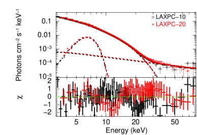
Figure 4: Top panel shows the best fit model and unfolded spectrum. The model used is nthComp+Gauss+PL (Model 1). The bottom panel shows residual in units of $\sigma$.

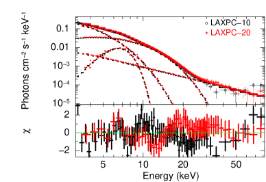
Figure 5: Top panel shows the best fit model and unfolded spectrum. The model used is diskbb+bbodyrad+Gauss+PL (Model 2). The bottom panel shows residual in units of $\sigma$.

A model consisting of emission from a multi-color disc, a blackbody component, a power-law and a broad iron line also provides statistically good description of the spectra (Model 2). This model has been used by Lin, Remillard and Homan (2010). To model the blackbody, we have used bbodyrad model in XSPEC which has normalization $N_{bb}$ = $(R_{km}/D_{10})^{2}$, where $R_{km}$ is the radius of the source in km and $D_{10}$ is distance to the source in units of 10 kpc. In Figure 4, we show the spectrum of the state ‘B1’ fitted with Model 1 and in Figure 5, we show the same fitted with Model 2. Best fit model parameters are listed in Table 2 (for Model 1) and in Table 3 (for Model 2). For both models, we use $N_{H}$ value fixed at 1.8 $\times$ 10²² cm^-2 (Lin, Remillard and Homan, 2010). Unless quoted the errors on the best fit spectral parameters are computed using $\Delta\chi^{2}$ = 1.0.

We also fit the spectra with diskline + nthComp + power-law model. Diskline model describes the broad iron line and takes into account the relativistic effects in the Schwarzschild metric (Fabian et al., 1989). We get a disc inclination $>$ 85^∘. Fitting the diskline model to the Chandra data of this source results in source inclination in the range $55-84$^∘ (Di Salvo et al., 2005). Hence, we fix the disc inclination at the highest value (84^∘) while fitting with this model. The best fit parameters for this model are listed in Table 4. We refer to this model as Model 3.

Figure 3: The Poisson noise subtracted power density spectra of 4U 1705-44 for various phases of banana state as marked in Figure 2. Each power spectrum corresponds to different states of B1 (a), B2 (b), B3 (c), B4 (d), B5 (e), B6 (f) and B7 (g) respectively. Solid line shows the best fit model.

4 Results

4.1 Timing Behaviour

The properties of PN and VLFN vary along the HID. The PN is centered at $\sim$ $1-13.5$ Hz. PN frequency does not show any clear correlation with the position on the HID. PN rms decreases from 7.1$\pm$0.23% to 1.87$\pm$0.61% as the source moves from B1 to B4 (see Table 1). As the source moves from B4 to B5, the PN component disappears and only power-law noise remains. At B6, it again appears with a much lower frequency of 0.95$\pm$0.26 Hz. As the source further moves to B7, the PN again disappears and PDS is dominated by a pure power-law noise (see Figure 3). The index of power-law component do not vary much along the HID. The power-law indices lie in the range of $1.56-2.03$ (see Table 1). The strength of VLFN is not correlated with the position on the banana branch.

Table 1: The best fit parameters obtained by fitting the PDS corresponding to seven segments of the HID. Power spectra of first four (B1, B2, B3, B4) and B6 segment are fitted with a Lorentzian plus power-law model and fifth and seventh segment (B5 and B7) are fitted with only a power-law model. We also give percentage rms in the frequency range $0.06-100$ Hz for Lorentzian and power-law components.

State	VLFN		Peaked-Noise (PN)			$\chi^{2}/dof$
	% rms	$\Gamma$	% rms	$\nu_{P}$ (Hz)	FWHM (Hz)
B1	2.82$\pm$0.58	2.03$\pm$0.19	7.10$\pm$0.23	12.58$\pm$0.14	7.62$\pm$0.36	70/62
B2	1.44$\pm$0.25	1.70$\pm$0.11	4.43$\pm$0.27	13.70$\pm$0.39	11.22$\pm$0.95	74/62
B3	1.52$\pm$0.40	1.87$\pm$0.21	2.63$\pm$0.79	10.66$\pm$0.63	7.99$\pm$4.1	114/62
B4	2.45$\pm$0.42	1.56$\pm$0.13	1.87$\pm$0.61	13.43$\pm$2.58	10.75$\pm$3.9	41/62
B5	1.45$\pm$0.36	1.63$\pm$0.17	-	-	-	48/62
B6	1.93$\pm$0.48	1.79$\pm$0.19	2.44$\pm$0.46	0.95$\pm$0.26	2.01$\pm$0.42	80/62
B7	1.81$\pm$0.30	1.75$\pm$0.12	-	-	-	82/62

Table 2: The best fit spectral parameters for the seven different parts of the HID of Model 1. $\Gamma_{nth}$ is the power-law photon index for nthComp, $kT_{e}$ is the electron temperature in keV and $N_{nth}$ is the normalization of nthComp. $\Gamma_{PL}$ is the photon index of power-law and $N_{PL}$ is the normalization of power-law. $E_{Fe}$ is the centroid energy of the iron line, $\sigma_{Fe}$ is the width of iron line, $\tau$ is the optical depth, $y-para$ is the Comptonization parameter. $F_{comp}$, $F_{PL}$ and $F_{tot}$ are flux of Comptonized component, flux of power-law component and total flux respectively. Fluxes are estimated in $0.1-100$ keV band and are in units of ergs/s/cm². EW is the equivalent width of the iron line in eV.

Parameters	B1	B2	B3	B4	B5	B6	B7
$\Gamma_{nth}$	2.10$\pm$0.01	2.10$\pm$0.02	2.05$\pm$0.04	1.98$\pm$0.03	1.96$\pm$0.02	1.88$\pm$0.02	1.72$\pm$0.03
kTe (keV)	2.71$\pm$0.03	2.69$\pm$0.03	2.62$\pm$0.05	2.57$\pm$0.04	2.59$\pm$0.04	2.57$\pm$0.04	2.50$\pm$0.02
$N_{nth}$	2.78 $\pm$0.07	1.04$\pm$0.03	0.19$\pm$0.11	0.90$\pm$0.11	1.09$\pm$0.05	1.91$\pm$0.08	0.66$\pm$0.06
$kT_{W}$ (keV)	0.18 (fixed)	0.46$\pm$0.05	0.91$\pm$0.09	0.49${}^{+0.27}_{-0.07}$	0.47$\pm$0.06	0.28 (fixed)	0.49$\pm$0.04
$\Gamma_{PL}$	0.86$\pm$0.21	0.79$\pm$0.13	3.41$\pm$ 0.03	2.51${}^{+0.56}_{-0.35}$	1.63$\pm$0.15	1.82$\pm$0.18	2.97$\pm$0.02
$N_{PL}$ $\times$ 102	0.17 $\pm$0.08	0.13 $\pm$0.06	746$\pm$51	38${}^{+92}_{-23}$	2.11$\pm$0.8	5.84$\pm$1.7	304$\pm$62
$E_{Fe}(keV)$	6.45$\pm$0.11	6.51$\pm$0.13	6.42$\pm$0.21	6.43$\pm$0.13	6.44$\pm$0.14	6.39$\pm$0.13	6.41$\pm$0.09
$\sigma_{Fe}$ (keV)	1.10$\pm$0.09	1.16$\pm$0.06	1.16$\pm$0.19	1.14$\pm$0.07	1.25$\pm$0.06	1.26$\pm$0.11	1.25$\pm$0.06
$E_{W}$ (eV)	369.5$\pm$30.8	425.9$\pm$25.5	406.2$\pm$38.1	460.7$\pm$27.60	511.5$\pm$20.4	488.7$\pm$28.6	501.4$\pm$29.8
$\tau$	9.78$\pm$0.09	9.82$\pm$0.17	10.32 $\pm$0.61	10.94$\pm$0.34	11.06$\pm$0.23	11.78$\pm$0.27	13.69$\pm$0.56
$y-$para	2.03$\pm$0.03	2.03$\pm$0.07	2.18$\pm$0.25	2.40$\pm$0.14	2.48$\pm$0.10	2.79$\pm$0.12	3.67$\pm$0.31
$R_{seed}(km)$	82.65$\pm$28.5	22.70$\pm$1.48	7.03$\pm$0.39	22.12$\pm$1.47	24.85$\pm$1.37	56.87$\pm$17.32	22.95$\pm$0.89
$F_{comp}$ $\times 10^{9}$	7.29$\pm$0.31	7.76$\pm$0.45	5.62$\pm$0.26	8.51$\pm$0.71	9.54$\pm$0.25	10.45$\pm$0.50	8.91$\pm$0.42
$F_{PL}$ $\times 10^{9}$	0.467$\pm$0.05	0.457 $\pm$0.04	3.01$\pm$0.29	0.676$\pm$0.27	0.371$\pm$0.05	0.586$\pm$0.07	2.55$\pm$0.12
$F_{tot}$ $\times 10^{9}$	7.97$\pm$0.35	8.48$\pm$0.55	8.89$\pm$0.39	9.53$\pm$0.76	10.04$\pm$0.25	11.47$\pm$0.49	11.89$\pm$0.43
$\chi^{2}/dof$	121/153	82/153	91/153	111/153	142/153	120/153	104/153

Table 3: The best fit spectral parameters of Model 2. $kT_{in}$ is the inner disc temperature in keV and $N_{dbb}$ is the normalization of diskbb component. $kT_{bb}$ is the blackbody temperature in keV and $N_{bb}$ is the normalization of blackbody. $\Gamma_{PL}$ is the photon power-law index and $N_{PL}$ is the normalization of power-law. $R_{in}$ and $R_{BB}$ are the inner disk radius and boundary layer radius respectively in units of km. $R_{eff}$ is the effective radius of inner disc in km. $F_{BB}$, $F_{dbb}$, $F_{PL}$, $F_{tot}$ are blackbody flux, disk flux, power-law flux and total flux respectively. Fluxes are estimated in $0.1-100$ keV band and are in units of ergs/s/cm².

Parameters	B1	B2	B3	B4	B5	B6	B7
$kT_{in}$ (keV)	1.18$\pm$0.03	1.28$\pm$0.04	1.78$\pm$0.14	1.68$\pm$0.08	1.62$\pm$0.10	1.56$\pm$0.11	1.73$\pm$0.12
$N_{dbb}$	170.5$\pm$18.5	133.4$\pm$16.5	25.8$\pm$8.3	35.3$\pm$8.6	45.89 $\pm$11.6	51.3$\pm$14.7	35.83$\pm$9.82
$kT_{bb}$ (keV)	2.18$\pm$0.02	2.22$\pm$0.03	2.41$\pm$0.08	2.33$\pm$0.05	2.33$\pm$0.04	2.30$\pm$0.04	2.38$\pm$0.05
$N_{bb}$	11.93$\pm$0.69	11.66$\pm$0.88	5.78$\pm$1.71	8.6$\pm$1.44	10.31$\pm$1.57	13.65$\pm$2.13	12.5$\pm$2.16
$\Gamma_{PL}$	1.74$\pm$0.21	1.62$\pm$0.26	3.29$\pm$0.11	3.20$\pm$ 0.15	2.90$\pm$0.20	2.83$\pm$0.16	2.98$\pm$0.11
$N_{PL}\times$ 102	4.8$\pm$2.1	2.9$\pm$1.1	508 $\pm$124	438$\pm$152	188$\pm$61	216$\pm$84	325$\pm$81
$R_{in}$ (km)	23.79$\pm$1.28	21.05$\pm$1.30	9.26$\pm$1.48	10.82$\pm$1.31	12.24$\pm$1.57	12.97$\pm$1.88	10.90$\pm$1.49
$R_{BB}$ (km)	2.59$\pm$0.075	2.56$\pm$0.09	1.80$\pm$0.27	2.19$\pm$0.18	2.40$\pm$0.18	2.77$\pm$0.21	2.65$\pm$0.22
$E_{Fe}$ (keV)	6.44$\pm$0.09	6.49$\pm$0.08	6.38$\pm$0.22	6.43$\pm$0.31	6.65$\pm$0.10	6.70$\pm$0.09	6.56$\pm$0.08
$\sigma_{Fe}(keV)$	1.30$\pm$0.06	1.31$\pm$0.09	1.19 $\pm$0.11	1.16$\pm$0.21	0.99$\pm$0.09	1.05$\pm$0.09	1.04$\pm$0.08
$R_{eff}$ (km)	68.77$\pm$3.72	60.83$\pm$3.76	26.77$\pm$4.30	31.27$\pm$3.84	35.39$\pm$4.55	37.48$\pm$5.44	31.52$\pm$4.30
$F_{BB}$ $\times 10^{9}$	2.88$\pm$0.13	3.01$\pm$0.12	2.08$\pm$0.31	2.71$\pm$0.26	3.23$\pm$0.39	3.98$\pm$0.38	4.07$\pm$0.45
$F_{dbb}$ $\times 10^{9}$	3.89$\pm$0.19	4.36$\pm$0.31	4.07$\pm$0.55	4.16$\pm$0.64	4.57$\pm$0.35	4.68$\pm$0.33	4.89$\pm$0.35
$F_{PL}$ $\times 10^{9}$	0.631$\pm$0.09	0.562$\pm$0.25	2.45$\pm$0.32	2.46$\pm$0.39	1.65$\pm$0.51	2.18$\pm$0.21	2.39$\pm$0.23
$F_{tot}$ $\times 10^{9}$	7.70$\pm$0.25	8.28 $\pm$0.39	8.90$\pm$0.88	9.66$\pm$ 1.15	9.74$\pm$0.68	11.16$\pm$0.55	11.70$\pm$0.67
$\chi^{2}/dof$	135/153	101/153	93/153	141/153	149/153	130/153	107/153

Table 4: The best fit spectral parameters of Model 3.

Parameters	B1	B2	B3	B4	B5	B6	B7
$R_{in}(GM/c^{2})$	6.0${}^{+0.33}_{-0.04}$	6.0${}^{+1.52}_{-0.05}$	6.0${}^{+2.64}_{-0.04}$	6.0${}^{+1.15}_{-0.05}$	6.0${}^{+0.65}_{-0.04}$	6.0${}^{+0.14}_{-0.03}$	6.0${}^{+0.18}_{-0.03}$
$E_{Fe}(keV)$	6.38$\pm$0.15	6.50$\pm$0.06	6.52$\pm$0.04	6.42$\pm$0.06	6.41$\pm$0.07	6.39$\pm$0.05	6.42$\pm$0.06
$\beta$	-2.31${}^{+0.07}_{-0.20}$	-2.27${}^{+0.08}_{-0.17}$	-2.44${}^{+0.13}_{-0.23}$	-2.37${}^{+0.07}_{-0.16}$	-2.43${}^{+0.06}_{-0.06}$	-2.44${}^{+0.09}_{-0.06}$	-2.44${}^{+0.05}_{-0.02}$
$\Gamma_{nth}$	2.10$\pm$0.02	2.11$\pm$0.03	2.11$\pm$0.07	1.99$\pm$0.04	1.98$\pm$0.02	1.88$\pm$0.02	1.77$\pm$0.05
$kT_{e}(keV)$	2.67$\pm$0.03	2.70$\pm$0.04	2.66$\pm$0.08	2.55$\pm$0.04	2.56$\pm$0.04	2.56$\pm$0.02	2.52$\pm$0.04
$kT_{W}$ (keV)	0.18 (fixed)	0.52$\pm$0.05	0.95$\pm$0.05	0.85${}^{+0.09}_{-0.31}$	0.55$\pm$0.02	0.30 (fixed)	0.86$\pm$0.15
$N_{nth}$	2.79$\pm$0.04	0.84$\pm$0.09	0.18$\pm$0.04	0.26$\pm$0.05	0.82$\pm$0.06	1.82$\pm$0.05	0.24$\pm$0.06
$\Gamma_{PL}$	0.97$\pm$0.17	0.87$\pm$0.25	3.43$\pm$0.09	3.29${}^{+0.08}_{-0.65}$	1.84$\pm$0.14	1.82$\pm$0.12	3.17$\pm$0.13
$N_{PL}\times 10^{2}$	0.27$\pm$0.09	0.18$\pm$0.11	748$\pm$128	567${}^{+146}_{-376}$	4.4$\pm$0.12	6.14$\pm$1.9	603$\pm$ 176
$\chi^{2}/dof$	123/152	83/152	95/152	113/152	149/152	132/152	108/152

4.2 Spectral Properties

In Figure 6, we show the variation of the best fit parameters of Model 1. The spectra consist of a thermal Comptonization component (nthComp), a power-law emission and a broad Gaussian line. The spectra of the source in the $3-80$ keV band do not require a soft thermal component and probably observation in the soft energy band ($<$ 3 keV) is required to observe this component. The parameters of nthComp are the electron temperature, power-law photon index and seed photon temperature. We assumed blackbody as the source of the seed photon. We note that the spectra during our observations were soft. The electron temperature $kT_{e}$ is in the range of $2.5-2.71$ keV. Fitting the data with this model gives the seed photon temperature of $0.45-0.9$ keV for B2, B3, B4, B5 and B7. However, the seed photon temperature for B1 and B6 can not be constrained and we need to fix it at the best fit value of 0.18 keV and 0.28 keV respectively.

The electron temperature shows subtle variations as the source moves from B1 to B7. The electron temperature $kT_{e}$ decreases from 2.71$\pm$0.03 keV to 2.50$\pm$0.02 keV as the source moves from B1 to B7. At the same time the spectral shape becomes harder and photon index $\Gamma_{nth}$ decreases from 2.10$\pm$0.01 to 1.72$\pm$0.03. We also derive the optical depth using the formula (Zdziarski et al., 1996),

$$\Gamma_{nth}=\left[\frac{9}{4}+\frac{m_{e}c^{2}}{kT_{e}\tau(1+\tau/3)}\right]^{\frac{1}{2}}-\frac{3}{2},$$ (3)

where, $m_{e}$ is the mass of the electron, $c$ is the speed of light in vacuum, $\tau$ is the optical depth. Here, the optical depth $\tau$ approximately equals the radial optical depth for a uniform spherical corona. The corona is found to be optically thick. The optical depth increases from 9.78$\pm$0.09 to 13.69$\pm$0.56 as the source moves from B1 to B7. The Comptonization parameter $y$, which is a measure of degree of Comptonization also increases from 2.03$\pm$0.03 to 3.67$\pm$0.31 as the source moves from B1 to B7.

The power-law observed during the soft state of the source 4U 1705-44 is variable and is present in all the seven spectra taken at different parts of the HID. The index of the power-law component varies between $0.79-3.41$ when we model the spectra with Model 1. The contribution of the power-law component to the total flux varies from 4 to 30% along the HID. However, it is not correlated with the position on the HID track.

The energy spectra have degeneracy and can also be described by diskbb+BB+PL+Gauss. In Figure 7, we plot the variation of the best fit spectral parameters of Model 2. The $\chi^{2}/dof$ is very similar for both models. The normalization of diskbb component $N_{dbb}$ varies between 25 to 170. The disk radius is connected with the normalization by formula, $N_{dbb}=(R_{in}/D_{10})^{2}\cos\theta$, where $R_{in}$ is the inner disk radius in km, $D_{10}$ is distance to the source in 10 kpc and $\theta$ is the disk inclination with respect to the observer. We give the derived disk radius $R_{in}$ assuming a source inclination of $80^{\circ}$ (as indicated by Model 3) and a distance of 7.4 kpc (Haberl and Titarchuk, 1995). The disk radius is in the range of $9-23$ km.

Shimura and Takahara (1995) suggested that if electron scattering modifies the spectrum from a standard disc, then diluted blackbody given by the equation,

$$F_{\nu}=\frac{\pi}{f_{col}^{4}}B_{\nu}(f_{col}T_{eff}),$$ (4)

approximates the local spectra. Here, $f_{col}$ is the spectral hardening or colour-correction factor and $T_{eff}$ is the effective temperature and $B_{\nu}$ is the Planck function. They found that the local spectrum can be described by a diluted blackbody with $f_{col}\sim$ 1.7 for 10% of Eddington luminosity. For a fully relativistic accretion disc and taking into account the bound-free process, Davis et al. (2005) derived the spectral hardening factor for different luminosities and inclination angles. For an inclination angle $i$ = 70^∘ and $L/L_{Edd}$ = 0.3, they obtained $f_{col}$ = 1.73 and for an inclination angle $i$ = 45^∘ and for same luminosity $f_{col}$ is $\sim$ 1.6. In our case, the total luminosity $L_{tot}$ is in the range of $0.3-0.5$ $L_{Edd}$. Hence, we take spectral hardening factor to be $\sim$ 1.7 to derive the disc radius. The effective temperature and effective inner disc radius is given by,

$$T_{eff}=T_{col}/f\quad and\quad R_{eff}=f^{2}R_{in}.$$ (5)

In Table 3, we also give effective radius of the inner disc. There may be an uncertainty in the inferred disk radius due to uncertainty in the disk inclination and the source distance. The photon index of power-law varies between $1.62-3.3$ when we model the spectra with Model 2. We also note that both flux and power-law index do not show any clear correlation with the position on the HID track.

We find that fitting the spectra of the HID sections of B1-B7 with Model 2 gives higher reduced $\chi^{2}$ compared to Model 1 (see Table 2 and Table 3). Therefore, Model 1 is a better description of the X-ray energy spectra of the atoll source 4U 1705-44 in the banana state than Model 2.

The Gaussian iron lines detected in the energy spectra are very broad (width $\sigma_{Fe}$ $\sim$ $1.0-1.3$ keV) and also strong (EW $\sim$ $369-$512 eV). We also note that modelling the $F_{e}$ line with diskline model (Model 3) gives a disc inclination $>$85^∘, which is higher than previously reported value (Di Salvo et al., 2005, 2009; Lin, Remillard and Homan, 2010; Piraino et al., 2016). If we freeze the inclination at 84^∘ then the inner disc radius approaches to the inner most circular orbit ($6GM/c^{2}$) where, G is the universal gravitational constant and M is mass of the central object (see Table 4). Note that inclination angle $>84^{\circ}$ does not improve the fit and a lower inclination worsen the fit. We also note that Model 3 which includes diskline component to model the iron line is not a better description of the data compared to Model 1 (see Table 4).

4.3 Correlation between parameters of spectra and Peaked noise

In order to understand the possible origin of the Peaked noise (PN), we correlate frequency of the PN with the parameters of Comptonization. Figure 8a shows the variation of the PN frequency vs $\tau$. There is no clear correlation between these two parameters. In Figure 8b, we show the variation of the PN frequency vs Comptonization flux. We find that the PN frequency is correlated with the Comptonization flux F_comp except the last point. In Figure 8c, we plot the PN frequency as a function of $kT_{e}$. No clear correlation is observed between these two parameters.

5 Discussion

We apply three different empirical models to describe the energy spectra of the atoll source 4U 1705-44 in the soft state observed during the GT phase of AstroSat mission. In first approach, Comptonization model of Zdziarski et al. (1996) describes the complex curvature in the soft state. However, in the second approach, we fit the spectral curvature with two thermal components: diskbb and BB. This approach has been adopted by Lin, Remillard and Homan (2010). First approach does not require a thermal component. Either the soft component may be inside the optically thick Corona and completely Comptonized, or it is peaking at lower energies and its contribution to the $3-80$ keV range is negligible.

Figure 6: Variation of the best fit spectral parameters and model fluxes of Model 1 along the HID. In the X-axis, 1, 2, 3, 4, 5, 6, 7 correspond to segments B1, B2, B3, B4, B5, B6 and B7 respectively. Model fluxes are in units of 10^-9 ergs/s/cm².

Figure 7: Variation of the best fit spectral parameters and fluxes of Model 2 along the HID. In the X-axis, 1, 2, 3, 4, 5, 6, 7 correspond to segments B1, B2, B3, B4, B5, B6, B7 respectively. Model fluxes are in units of 10^-9 ergs/s/cm².

By fitting the spectra with the Comptonization model, we find that the corona is cool and optically thick ($\tau\sim 10-14$). If this corona covers the NS surface then soft BB photons emitted from the boundary layer will be Comptonized. The enhancement of seed photon luminosity by scattering in an optically thick Compton cloud is given by $3kT_{e}/kT_{seed}$ (Dermer, Liang and Canfield, 1991). The electron temperature of the corona is $\sim$ 3 keV. We have assumed source of the seed photon as a blackbody emission from the surface of NS. We get luminosity enhancement factor $\eta\sim$ $8-42$. The seed photon flux $F_{seed}$ will be $F_{Comp}/\eta$. In Table 2, we give the NS radius derived from this seed photon flux assuming an isotropic luminosity. The derived radius is in the range of $7-80$ km. Here, we have assumed a spherical corona around the NS. However, it could be transition layer between the NS surface and accretion disc (Titarchuk et al., 2001) or Accretion Disc Corona (ADC) above the disc (Church et al., 2014). Moreover, we could be able to constrain the variation in the properties of the corona e.g. temperature and optical depth. We find that as the source intensity increases, optical depth of the corona also increases. Most probably radiation pressure drives matter from the accretion disc to the larger corona or ADC (Agrawal and Sreekumar, 2003) and hence increases its density. As the optical depth of the corona increases, the photons suffer more number of scatterings and hence in turn causes a decrease in the corona temperature. The above scenario explains the decrease in the temperature of the corona as the source moves from B1 to B7.

Fitting the data with the model adopted by Lin, Remillard and Homan (2010) also provides a statistically good description of the spectra. The inner-disc temperature varies between $1.20-1.80$ keV as the source moves along the banana track. The effective inner disc radius $R_{eff}$ varies from $26-70$ km, assuming spectral hardening factor $f_{col}=1.7$.

The boundary layer emission is modeled as blackbody. The NS radius obtained is very small $\sim$ 2 km (see Table 3). The radius of NS is obtained assuming that the NS boundary layer emits isotropically. However, the boundary layer may not emit isotropically. Lin, Remillard and Homan (2010) suggested that emission area of the boundary layer is $\sim$ 20% of the NS surface area (for inclination $i$ = 25^∘). This will increase the NS radius by a factor of 2.25 times and still gives smaller values of NS radius ($\sim$ 5 km). Even smaller size of the boundary layer depends on the radiative transfer processes in the NS atmosphere (Popham and Sunyaev, 2001; Lin, Remillard and Homan, 2010) and the spectral hardening factor due to free-free and bound-free processes. The radius of NS/Bounadry layer ($R_{seed}$) estimated using Model 1 is much closer to the expected NS radius compared to that estimated from Model 2 (see Table 2 and Table 3).

Figure 8: Correlation between the spectral parameters and the best fit PN frequency. Left plot (a) shows correlation between the optical depth $\tau$ and $\nu_{PN}$. Centre plot (b) shows correlation between $\nu_{PN}$ and the Comptonization flux, where as right plot (c) shows correlation between kTe and $\nu_{PN}$. See text for details.

In all seven parts of the HID (marked in Figure 2), we find the presence of a power-law tail in the energy spectra. During our observations, the source was in the soft spectral state. The source has also shown a hard tail during the BeppoSAX observations (Piraino et al., 2007, 2016) and Suzaku observations. During these observations, the source was also in the soft state (see Piraino et al. 2007; Lin et al 2010). A power-law tail has been previously reported in atoll sources 4U 1728-34 (Tarana et al., 2011) and 4U 1636-536 (Fiocchi et al., 2006) and Z-sources GX 17+2 (Di Salvo et al., 2000), Sco X-1 (D’Amico et al., 2001), GX 349+2 (Di Salvo et al., 2001) and Cyg X-2 (Di Salvo et al., 2002).

The contribution of the power-law component to the total flux is around $4-30$% (for Model 1). The flux does not show any clear correlation with the position on the banana pattern. The flux was highest (30%) at the B3. There are many competing models to explain the origin of the non-thermal component. Such a hard tail can be produced in either, hybrid thermal/non-thermal population of electrons in the corona (Poutanen & Coppi, 1998) or Comptonization in bulk motion of matter close to the compact object (Ebisawa, Titarchuk & Chakrabarti, 1996; Titarchuk and Zannias, 1998). However, Farinelli, Titarchuk & Frontera (2007) suggested that at a high accretion rate, radiation pressure due to emission from the neutron star surface can slow down the bulk motion of matter causing quenching of bulk Comptonization. Other possible mechanisms which have been proposed to explain the non-thermal tails are, Comptonization of the seed photons in a relativistic jet (Di Salvo et al., 2000) or synchrotron emission from such a jet.

A broad iron line ($FWHM\sim$ 2 keV) is present in all the spectra. Both diskline and a broad Gaussian line models provide equally good description of the iron line feature. This suggests that probably, smearing of the feature in a relativistic accretion disc account for the broadening. An alternative mechanism, broadening by thermal Comptonization of the line emission in a corona surrounding the disc can also explain the large width (see Di Salvo et al. 2005). In this case, line width is given by (Kallman and White, 1989; Brandt and Matt, 1994),

$$\sigma_{Fe}=0.02E_{Fe}\tau(1+0.78kT_{e}).$$ (6)

In the present case, average temperature of the corona is $\sim$ 2.7 keV and the line energy is $\sim$ 6.5 keV. The line width is in the range of $1.10-1.25$ keV (for Model 1). Hence, the Fe line is broadened in the corona having optical depth $\sim$ $2.7-3.2$. Therefore, most probably the line is produced in the external parts of the corona. Since in the present case the optical depth is very high ($\tau\sim$ $10-14$), the Fe-line produced at the inner part of the corona will be completely smeared.

Correlated spectral and fast timing properties of this source have been studied in detail by Olive, Barret and Gierlinski (2003) using the RXTE-PCA data. In the soft state, they found low frequency noise (LFN) component centered at $\sim$ $35-45$ Hz. VLFN was detected in one of the observations in the soft state. We detect a broad feature at $1-13$ Hz (PN) in the B1, B2, B3 and B4 and B6 state. The integrated rms of this feature varies between $1.87-7.1$%, which is lower compared to that of the LFN. The percentage rms of the LFN in the high soft state varies between $5-12.5$%. The PN frequencies (B1-B4) show correlation with the total Comptonization flux in the $0.1-100$ keV band. Olive, Barret and Gierlinski (2003) found that the LFN frequency is anti-correlated with the hard flux in the $20-200$ keV band. However, we find that at B6 though Comptonization is strong frequency is low. We choose integrated Comptonized flux instead of $20-200$ keV flux because it is a better measure of strength of the corona. If this feature is produced by oscillations in the corona, then it is expected that as the corona becomes compact and cool, characteristic frequency of the oscillation may also increase. But we find that the observed correlation between the spectral and temporal properties is not consistent with this expected behaviour. However, detection of the PN in the $3-20$ keV band where the Comptonized emission is dominant suggests that the PN is linked with the corona. It is also possible that the PN is produced in the disc and modified in the corona as suggested by Swank (2001) to explain the low-frequency QPOs in the blackhole candidates. A correlation between the disc flux and the PN parameters will shed more light on this.

6 Conclusion

In this work, we present a detailed spectral and timing analysis of the source 4U 1705-44 using LAXPC/AstroSat data. The source traced a banana pattern in the HID during the LAXPC observations. We fit the spectra with three different approaches. We suggest that the model consisting of Comptonized emission from the corona (Model 1) is a better description of the spectra in the banana state. The spectra show presence of a variable hard tail and a broad iron line centered at $6.4-6.7$ keV. Our analysis suggests that the broad iron line is most probably produced at the outer part of the corona with an optical depth in the range of $2.7-3.2$. We also investigate the evolution of the spectral parameters along the HID. We find that the optical depth of the corona increases and the electron temperature decreases as the source moves along the banana branch. Non-thermal component does not show any clear correlation with the position on the HID. In the PDS, we find a broad PN component (with a quality factor Q $\sim$ $0.48-1.65$) centered at $1-13$ Hz. The PN is detected in the energy band where Comptonization is the main process, which suggests that the origin of the PN is linked with the corona. However, correlation between the disc/thermal flux and the PN frequency is required in order to understand the mechanisms producing the broad PN in the power spectra of this source.

References

- Agrawal et al. (2017) Agrawal P.C.,Yadav J.S.,Antia H.M.,Dedhia Dhiraj, Chauhan Jai Verdhan, Manchanda R.K., Chitnis V.R. et al.,2017,JApA,38,30
- Agrawal and Misra (2009) Agrawal V.K., Misra R., 2009,MNRAS,398,1352
- Agrawal and Sreekumar (2003) Agrawal V.K., Sreekumar P., 2003,MNRAS,346,933
- Antia et al. (2017) Antia H.M., Yadav J.S, Agrawal P.C, Verdhan Chauhan Jai, Manchanda R.K.,Chitnis Varsha, Paul B., Dedhia Dhiraj et al.,2017,ApJS,231,10
- Barret (2001) Barret D., 2001,AdSpR,28,307
- Barret et al. (2000) Barret D., Olive J.F., Boirin L.,Done C.,Skinner G.K, Grindlay J.E., 2000,ApJ, 533,329
- Berger and van der Klis (1998) Berger M. and Van der Klis N., 1998,A&A, 340,143,
- Brandt and Matt (1994) Brandt W.M.,& Matt G., 1994,MNRAS,268,1051
- Church et al. (2014) Church M.J., Gibiec A., Balucinska-Church M., 2014,MNRAS,438,278
- Davis et al. (2005) Davis S.W., Blaes O.M., Hubeny I.,Turner N.J.,2005,ApJ,621,372
- D’Amico et al. (2001) D’Amico F.,Heindl W.A.,Rothschild R.E., Gruber D.E., 2001, ApJ, 547,L147
- Dermer, Liang and Canfield (1991) Dermer C.D., Liang E.P., Canfield E., 1991,ApJ,369,410
- Di Salvo et al. (2000) Di Salvo T., Stella L.,Robba N.R., van der Klis M., Burderi L., Israel G.L, Homan J.,Compana S. et al., 2000, ApJ, 544, L119
- Di Salvo et al. (2001) Di Salvo T., et al., 2001,ApJ,554,49
- Di Salvo et al. (2002) Di Salvo T. et al., 2002, A&A, 386, 535
- Di Salvo et al. (2005) Di Salvo T., Iaria R.,Mendez M., Burderi L., Lavagetto G.,Robba N.R., Stella L.,van der Klis M., ApJ,623,L121
- Di Salvo et al. (2009) Di Salvo T., D’Ai A., Iaria R., Burderi L., Dovciak M., Karas V., Matt G., Papitto A., et al., 2009,MNRAS, 398,2022
- Di Salvo et al. (2015) Di Salvo T., Iaria R., Matranga M., Burderi L., D’Ai A., Egron E., Papitto A., Riggio A.,Robba N.R. et al.,2015,MNRAS,449,279
- Done et al. (2007) Done C., Gierlinski M., Kubota A., 2007, A&A Rev., 15,1
- Ebisawa, Titarchuk & Chakrabarti (1996) Ebisawa K., Titarchuk L., & Chakrabarti S.K.,1996,PASJ,48,59
- Fabian et al. (1989) Fabian A.C., Rees M. J., Stella L., & White N.E., 1989,MNRAS, 238, 729
- Farinelli, Titarchuk & Frontera (2007) Farinelli R., Titarchuk L., & Frontera F., 2007, ApJ, 662,1167
- Fiocchi et al. (2006) Fioochi M., Bazzano A., Ubertini P., 2006, ApJ, 651,416
- Ford, van der Klis and Kaaret (1998) Ford E.C., van der Klis M. and Kaaret P.,1998,ApJ,498,L41
- Gottwald and Haberl (1989) Gottwald M. and Haberl F.,1989,339,1044
- Haberl and Titarchuk (1995) Haberl F., and Titarchuk L.,1995,A&A,299,414
- Homan et al. (2007) Homan J., van der Klis M., Wijnands R., Belloni,T., Fender R., Klein-Wolt, M., Casella P., Mendez M., et al., 2007, ApJ, 656,420
- Hasinger and van der Klis (1989) Hasinger G., van der Klis M., 1989, A&A, 225, 79
- Kuulkers et al. (1994) Kuulkers E., et al., 1994,A&A,289,795
- Kallman and White (1989) Kallman T., & White N.E., 1989, ApJ, 341,955
- Lin, Remillard and Homan (2009) Lin D., Remillard R.A. and Homan J.,2009,ApJ, 696,1257
- Lin, Remillard and Homan (2010) Lin D., Remillard,R., Homan J.,2010,ApJ,719,1350
- Lin, Remillard and Homan (2007) Lin D., Remillard R., Homan J.,2007,ApJ,667,1073
- Mitsuda et al. (1984) Mitsuda K., et al., 1984, PASJ, 36, 741
- Olive, Barret and Gierlinski (2003) Olive J.F., Barret D., Gierlinski M,2003,ApJ, 583,416
- Piraino et al. (2007) Piraino S., Santangelo A., Di Salvo,T, Kaaret P.,Horns D., Iaria R., and Burderi L.,2007,A&A,471,L17.
- Piraino et al. (2016) Piraino S., Santangelo A., Muck B., Kaaret P., Di Salvo T.,D’Ai,A. Iaria R.,Egron E.,2016,A&A,591,A41
- Popham and Sunyaev (2001) Popham R., & Sunyaev R., 2001,APJ,547,355
- Remillard et al. (2006) Remillard R.A.,& Lin D., The ASM Team at MIT and NASA/GSFC 2006, Astron. Tel. 696