Influence of the Solar Global Magnetic Field Structure Evolution on CMEs

Abstract

The paper considers the influence of the solar global magnetic field structure (GMFS) cycle evolution on the occurrence rate and parameters of coronal mass ejections (CMEs) in cycles 23-24. It has been shown that over solar cycles, CMEs are not distributed randomly, but they are regulated by evolutionary changes in the GMFS. It is proposed, that the generation of magnetic Rossby waves in the solar tachocline results in the GMFS cycle changes. Each Rossby wave period favors a particular GMFS. It is proposed that the changes in wave periods result in the GMFS reorganization and consequently in CME location, occurrence rate, and parameter changes. The CME rate and parameters depend on the sharpness of the GMFS changes, the strength of the global magnetic field and the phase of a cycle.

1 Introduction

CMEs are the most energetic solar activity phenomena. They have speeds up to $\sim 10^{3}$ km s^-1, total mass of $\sim 10^{16}$ g, and energy reaching $\sim 10^{23}-10^{25}$ erg (Howard1985; Cyr2000; Gopalswamy2006). CMEs are considered to be associated with large-scale, closed magnetic field structures in the solar corona (Hundhausen1993; Munro1979; Chen2000; Forbes2006; Gopalswamy2006). They are caused by loss of equilibrium of the pre-existing magnetic structure [Schmieder (2006)]. Significant parts of the solar atmosphere are involved in a CME. CMEs are known to be the main drivers of space weather [Schwenn (2006)]. Ejected coronal plasma may cause strong geomagnetic storms. CME source regions can be identified with different types of large-scale structures(Hundhausen1993; Khan2000; Bemporad2005; Zhou2006). CMEs may be caused by the instability or lack of equilibrium in coronal loops (McAllister1996; Zhou2006; Lara2008; Harrison2010). Some observations have shown that CMEs are associated with streamers (Illing1986; Steinolfson1988; Hiei1993; Hundhausen1993; Subramanian1999; Floyd2014). Other investigators relate CMEs to coronal holes (Hewish1986; Bilenko2009) or sigmoid magnetic field structures [Sterling et al. (2000)]. The initiations of CMEs are often found to be related to the other solar activity, e.g., active regions (ARs), flares, filaments/prominences, streamers, and coronal holes or in different combinations.

On the whole, the CME activity tends to track a solar cycle (Webb1991; Webb1994; Hildner1976; Cyr2000; Gopalswamy2006; Cremades2007; Robbrecht2009a; Gerontidou2010; Lamy2014), but it differs in a significant way from that of the small scale solar activity phenomena due to the fact it is more in line with the evolution of the global magnetic field (Li2009; Bilenko2012). The changes in the distribution of CME latitudes do not correspond to those related to small scale magnetic structures such as sun spots or $H\alpha$ flares; they resemble those related to large-scale magnetic structures, such as prominences and bright coronal regions [Hundhausen (1993)]. During cycle 23 the CME activity shows a significant peak delay with respect to the AR cycle [Robbrecht, Berghmans, and Van der Linden (2009)]. Large-scale solar magnetic fields have a significant effect on the characteristics and propagation of CMEs [Fainshtein and Ivanov (2010)]. Different CME parameters have different behavior in solar cycle maxima and minima (Hundhausen1993; Hundhausen1994; Vourlidas2010; Vourlidas2011; Bilenko2012). This reflects their association with different shapes and orientation of the closed structures of the solar magnetic field at different phases of a solar cycle [Bravo, Blanco-Cano, and Nikiforova (1998)] and the influence of the solar global magnetic field cycle evolution (Bilenko2012; Petrie2013). The changes in the domination of the sectorial and zonal structures of the solar global magnetic field influence the CME rate and parameters. During the zonal structure domination, the solar minima phases, CMEs have lower occurrence rate and parameters on average. When sectorial structures begin to dominate at the rising phase of solar activity, the sharp increase in CME daily rate and parameters is observed. The latitudinal distribution and the statistics of CME parameters are also different for periods of zonal and sectorial structure domination [Bilenko (2012)]. In Petrie2013 it was shown that the rate of solar eruptions was higher for years 2003-2012 than for years 1997-2002. This was explained by the weakness of the late-cycle 23 polar fields and the influence of the changes in the polar fields on the global coronal field structure.

Comparing the occurrence rates of CMEs with the long-term evolution of the global white light coronal density distribution Sime1989 concluded that CMEs arise from pre-existing magnetic structures which become stressed by the global magnetic field rearrangement to the point of instability. CMEs are believed to be a consequence of the coronal field rearrangement due to a loss of stability of the magnetic field [Forbes (2000)]. CMEs are the result of a global magnetohydrodynamic process and represent a significant restructuring or reconfiguring of the global coronal magnetic field (Harrison1990; Low1996). The topology changes from closed to open magnetic field configuration result in CMEs [Wen et al. (2006)]. And vice versa CMEs can have influence on the coronal magnetic field reconfiguration [Liu et al. (2009)]. Low (1996, 2001) suggested that CMEs can be a basic mechanism of coronal magnetic field reconfiguration. However, in Alexander1996 and Zhao1996 it was shown that CMEs did not greatly affect the large-scale coronal structure and the neutral sheet geometry. Using numerical modeling, Luhmann1998 have shown that coronal field lines can be opened without significant changes in the coronal structure and the neutral line. Subramanian1999 have found that although 63% of CMEs from January 1996 to June 1998 were associated with streamers, the most of CMEs had no effect on the streamer. The lifetime of the changes in the heliospheric current sheet (HCS) location caused by CMEs were found to be significantly less than the lifetime of the HCS structure even during solar maximum Zhao and Hoeksema (1996).

According to Ivanov1997 both the properties of CMEs and their cyclic evolution are closely related to the multipole component of the global solar magnetic field ($n>4$), corresponding to a system of closed magnetic fields on the Sun with characteristic mean dimensions $D>40^{\circ}$. CMEs are caused by the interaction of two large-scale field systems, one of them (the global field system) determines the location of CMEs and another (the system of closed magnetic fields) their occurrence rate Ivanov et al. (1999). In Obridko2012 it was established that CME velocity and occurrence rate depend on the cyclic variations of the large-scale magnetic fields which determine active complex evolution and are responsible for the occurrence of major CMEs. Equatorially trapped Rossby-type waves were proposed by Lou2003 as large-scale quasi-periodic source of the photospheric magnetic field disturbances, resulting in observed CME periodicities.

While it has been considered that CMEs are a part of the large-scale magnetic field evolution this connection has not been investigated in detail. In this paper, the relevance of the CME occurrence rate and parameters to the GMFS cycle evolution, and their association with magnetic field oscillations has been analyzed. The GMFS changes, as a consequence of the excitation of Rossby waves of different periods and the influence of the changes in Rossby wave periods on GMFS reorganization and consecutively on the CME rate and parameters during solar cycles 23 and 24, are discussed. The comparison with AR parameter cycle evolution is also studied.

The structure of the paper is as follows. Section secdata describes the used data. In Section secglobmag the GMFS cycle evolution is analyzed. In Section seccme CME rate and parameter cycle changes have been described and the comparison with that of GMFS and the oscillations in the mean solar magnetic field, as well as the comparison with AR parameter cycle evolution, is made. The results are discussed in Section secdiscus.The main conclusions are listed in Section seccon.

2 Data

secdata

The data from the Large Angle and Spectrometric Coronagraph (LASCO) on board the Solar and Heliospheric Observatory (SOHO) Brueckner et al. (1995) was used. For each CME event, the SOHO/LASCO CDAW CME catalogue gives position angle, plane-of-sky speeds and width, acceleration, mass and energy. Details on the CME catalog can be found in Yashiro2004 and Gopalswamy2009. There were data gaps in SOHO for June-October 1998 and January-February 1999. In this catalog CME masses and potential energies may be underestimated by a maximum of two times, and the kinetic energies by a maximum of eight times (Vourlidas2010, 2011). In Yashiro2008 it was noted that some slow and narrow CMEs may not be visible when they originate from the solar disc centre. Due to projection effects, some low-latitude (high-latitude) CMEs may be misidentified as high-latitude (low-latitude) CMEs, but no plane-of-sky CME parameter correction was made, because according to Howard2008, in a large sample of events, plane-of-sky measurements may be suitable for studies of general trends. Correcting for projection effects is necessary for those investigations that deal with the properties of individual CMEs.

To analyze the solar global magnetic field, the data on the mean solar magnetic field (MMF) and source surface synoptic maps from the Wilcox Solar Observatory (WSO) were used. For these maps, the coronal magnetic field is calculated from photospheric fields with a potential field model with the source surface location at 2.5 solar radii (Altschuler1969; Altschuler1975; Altschuler1977; Schatten1969; Hoeksema1986; Hoeksema1988; Wang1992). Source surface magnetic field data are consist of $30$ data points in equal steps of sine latitude from $+70^{\circ}$ to $-70^{\circ}$. Longitude is presented in $5^{\circ}$ intervals.

For comparison with AR parameter cycle evolution, Space Weather Prediction Center data were used.

3 Global magnetic field structure evolution

secglobmag

Unfortunately, direct methods to measure the magnetic field in the solar corona during solar cycles, especially in its quiet regions, are unavailable to date. Therefore, the WSO calculation results on coronal magnetic fields in the potential-field approximation with a standard spherical source surface at 2.5 solar radii (PFSS) for Carrington rotations (CRs) 1905 - 2119 were employed. The PFSS model provides remarkably good description of the coronal magnetic field structure. The longitudinal distribution of positive-polarity and negative-polarity magnetic fields, resulting from the PFSS extrapolation at 2.5 solar radii, is displayed in Figure londiaga. The times of sunspot maximum and minima are marked at the top of the Figure londiaga. Changes in the magnetic fields at the source surface reflect those observed over the same time in the photosphere. The magnetic structure of the Sun as a star is known to be in good agreement with the PFSS extrapolation of the coronal magnetic field Kotov (1994). In Figure londiagb the longitudinal diagram of the photospheric magnetic field of the Sun as a star, composed from the data of the solar MMF, is presented. In Figures londiaga and londiagb colors show the distribution of positive-polarity (yellow-red) and negative-polarity (blue-lilac) magnetic fields averaged over latitude for each CR. The brightness at a certain point is proportional to the magnetic field strength. Black color marks the missing data.

In the diagrams, Y-axis denotes longitude in degree and X-axis denotes CR. Each thin vertical bar shows magnetic field distribution for each CR. When there are two longitudinal intervals one covered by the positive-polarity magnetic fields and the other covered by the negative-polarity ones in one CR (along Y-axis), it means that the two-polarity structure is observed and when there are two longitudinal intervals covered by positive-polarity magnetic fields and two longitudinal intervals covered by negative-polarity magnetic fields in one CR (along Y-axis), it means that a four-sector structure exists during the CR. The periods corresponding to the two-sector and four-sector structures are marked in the Figure londiag as 2s (two-sector structure) and 4s (four-sector structure). When the polarity changes from one CR to the next (along the X-axis) in some longitudinal intervals (Y-axis) it means that the structure changes its polarity.

The structures in Figures londiaga and londiagb display a good agreement. Thus, the positive-negative-polarity structure is believed to trace the global solar magnetic field evolution from the photosphere to the corona. The diagrams show that positive-polarity and negative-polarity magnetic fields are not distributed randomly, but rather, form a multi-scale GMFS, depending on the phase of cycles 23 and 24. Similar structures were also observed in cycles 21 and 22 (Hoeksema1988; Hoeksema1991; Levine1979; Kovalenko1988).

From Figures londiaga and londiagb it is seen that the lifetime of each sector structure is different during different cycle phases. During the minimum of the cycle 23 the lifetime of the observed structures was short approximately 3-5 CRs that was $\sim 80-135$ days. During the maximum, the declining phase of cycle 23, and the minimum of cycle 24 the lifetime of each structure ranged from $\sim 10$ CRs to $\sim 1970$ CRs that was from 270 days to $\sim 5$ years. A closer look at Figures londiaga and londiagb reveals periods of slow and fast GMFS changes. There were two fast ($\sim 1-3$ CRs) redistributions of the GMFS, covering a considerable part of the solar surface during the maximum and the beginning of the declining phase of cycle 23. Two-sector structure with the positive-polarity field domination at longitudes $330^{\circ}-360^{\circ}-0^{\circ}-140^{\circ}$ and the negative field at longitudes $140^{\circ}-330^{\circ}$ was existing from CR 1959 until CR 1969. The global picture remained quasi-stable during $\sim 300$ days. Then the polarity structure was reversed during one CR. A new two-sector structure with the opposite distribution of the positive-polarity and negative-polarity magnetic fields existed during 10 CRs ($\sim 0.75$ year) from CR 1970 until CR 1980, and then in CR 1980 the polarity structure was reversed to the previous distribution of the positive-polarity and negative-polarity magnetic fields in one CR. Such redistributions of the GMFS involve the whole Sun. Magnetic structures were also observed from CR 1905 to 1950 (the minimum and the rising phase of cycle 23). However, their scale in longitude and in time was somewhat smaller compared to those of the maximum and the declining phase.

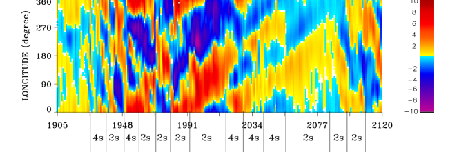
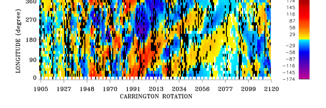
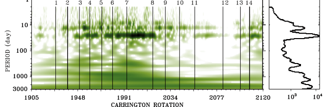
Figure 1.: (a) The longitudinal diagram of coronal magnetic field evolution resulting from the PFSS extrapolation at 2.5 solar radii. (b) The longitudinal diagram of the magnetic field of the Sun as a star. Yellow-red colors denote positive-polarity magnetic fields and blue-lilac - negative-polarity fields. Black marks the missing data. (c) Wavelet power spectrum of the mean solar magnetic field.londiag

Why the structures form and disappear and what controls the regularity in their evolution is not yet understood. Obviously, the observed distribution and redistribution of magnetic fields are the consequence of the processes occurring inside the Sun. Gilman (1969b, 1969a) was the first to propose that observed solar magnetic fields can be the result of Rossby waves in the Sun’s convection zone and photosphere.

The wavelet power spectrum of the daily MMF is shown in Figure londiagc. To obtain values of the periods (frequencies) of oscillations contained in the time series it is necessary to use any method of decomposition of this time series. Fourier analysis provides the values of the periods (frequencies) only. The wavelet technique allows obtaining not only values of periods contained in the analyzed time series, but it also shows the period’s location in time. Thus, we can see when certain periods appear and disappear. In our case it allows us to compare the evolutionary changes in the GMFS with periods of oscillations in the observed magnetic field of the Sun as a star. Morlet wavelet technique was used. We see oscillations with different periods during different solar cycle phases. The wave periods became shorter from $\sim$400 d to 50 d from the minimum to the maximum of cycle 23, and they grew to the minimum of cycle 24 again. The process was not a smooth one, but it had a form of individual steps. Each period remained quasi-constant until a new one appeared. The periods of $\sim$13 d and $\sim$27 d can be associated with the photospheric magnetic fields and ARs Bai (1990). The periods of waves that can be associated with the GMFS in Figures londiaga and londiagb lie in the range $\sim$50 d - 1000 d (Figures londiagc). The significant reconfigurations of the GMFS, observed in Figures londiaga and londiagb, are marked by thin vertical lines. We can see that the changes in the GMFS are accompanied by the changes in the periods of oscillations that each wave period coincides in time with a particular GMFS distribution. Periods from 40 to 600 days do not exist all the time, but they appear and disappear. They strengthen in the periods of $\sim 200\div 400$ d from CR 1938 (line 2) to CR 1959 (line 4) coinciding with the formation of the large GMFS. The appearance of periods $\sim 80\div 110$ d line 3 occur when a two-sector structure was changed to a four-sector structure, and these periods disappear at the time marked by the line 4 (CR 1959). The periods became shorter $\sim 50\div 90$ d and $\sim 100\div 200$ d and the GMFS changed from four-sector to two-sector. The first periods disappear before the line 5 and the second one at the time marked by line 6. It is interesting to note that the disappearance of the first periods coincide in time with the formation of the small negative-polarity feature inside the positive-polarity pattern at longitudes $\sim 40^{\circ}\div 80^{\circ}$. From CR 1970 (line 5) the periods of $\sim 50\div 90$ d disappeared and the waves with periods $\sim 80\div 120$ d appeared, and the GMFS reversed its polarity. Since CR 1980 (line 6), the periods of $\sim 50\div 100$ d and $\sim 120\div 200$ d appeared again and the GMFS also reversed its polarity to the previous state. Line 6 marks the moment when two-sector structure reverses it’s polarity. The periods of $\sim 50\div 70$ d appeared and their disappearance coincide with formation of extensions from the positive-polarity patterns at CR $\sim$1980 (line 6). From CR 1993 (line 7) the periods became longer stepwise and the large-scale two-sector drifting structure was observed. The drift in the GMFS means the changes in the differential rotation. The periods of $\sim 40\div 70$ d, appearing at the time marked by line 7, may coincide with the formation of an extension of large-scale positive-polarity pattern at longitudes $\sim 160^{\circ}\div 200^{\circ}$. The GMFS from CRs 1980 to 2020 was associated with the same periods as the GMFS of CRs $\sim 1949-1970$. Since CR 2017 (line 8), the GMFS became a four-sector drifting structure, and at the same time we can see step-like lowering periods, which can be associated with that structure in the wavelet spectrum. At the rising phase of cycle 24 the new periods appeared in the wavelet power spectrum, and at the same time the GMFS changed its drift direction. The intensity of the cycle 24 period was lower than that of cycle 23.

As well as being an interesting phenomenon in its own right, this behavior of the solar global magnetic field may shed new light on the observed regularity in CME formation and rate and parameter evolution during solar cycles. To quantify the changes in the GMFS, the CR average magnetic field strength of the positive-polarity and negative-polarity magnetic fields and their absolute value sum were calculated (Figure globkoefa) using the longitudinal diagram (Figure londiaga). In Figure londiagb the CR average magnetic field strength of the positive-polarity and negative-polarity magnetic fields and their absolute value sum for the magnetic fields of the Sun as a star is presented. It is seen that the behavior of magnetic fields in Figures londiaga and londiagb is identical. The intensity of the magnetic field was low at the minima of cycles 23 and 24. Toward the maxima, the magnetic field strength increased. The magnetic field strength decreased during the reorganizations of the GMFS (thin vertical lines in Figures globkoefa and globkoefb). In each pattern, the magnetic field strength did not grow gradually, but underwent abrupt changes, reflecting changes in activity within a pattern.

Figure 2.: (a) Magnetic field strength from the longitudinal diagram; (b) $K_{lon}$; (c) $K_{c}$; (d) $K_{u}$. Thin vertical lines mark the moments of change in the GMFS.globkoef

In order to describe the phenomenon of longitudinal structure changes quantitatively, a series of $K_{lon}$ coefficient was built Bilenko (2012). In the longitudinal diagram, magnetic field polarity in each CR was compared with the successive CR polarity. The number of points at which the polarity changed was summed up. Then it was normalized to the total number of longitudinal points in CR so that $K_{lon}$ takes value from 0 to 1 for each CR. Such normalization allows us to compare the GMFS change rate at different solar cycle phases.

$$K_{lon}=\frac{\sum\limits_{i=0}^{n}{L_{chi}}}{n}$$ (1)

where $L_{chi}$ is the number of longitudes where polarity was changed between two successive CRs, $n$ - the total number of longitude points in CR ($n=72$). Figure globkoefc presents the $K_{lon}$ coefficient evolution. The amplitude of $K_{lon}$ decreased up to 0 during the maximum and the decline phase of cycle 23 when the large quasi-stable structures were existing. The amplitude of $K_{lon}$ reaches $\sim 0.74$ during the periods of small structures and sharp changes in GMFS. The peaks in $K_{lon}$ denote the moments of the GMFS reorganization. Thin vertical lines are drawn through these peaks and the thin vertical lines in all Figures correspond to these peaks in $K_{lon}$.

To evaluate the total rate of the magnetic field polarity changes, the coefficient $K_{c}$ was calculated (Figure globkoefd) from the comparison of polarity in each point in successive source surface magnetic field maps (WSO). It was normalized to the total number of points in a map.

$$K_{c}=\frac{\sum\limits_{i=0}^{k}P_{i}}{k},$$ (2)

where $P_{i}$ is the number of map points where polarity was changed, $k$ - the total number of points in a map ($k=2160$). $K_{c}$ reflects the rate of a new magnetic flux emergence.

4 CME Evolution

seccme

White light coronagraphs LASCO have observed nearly 17859 CMEs from 1996 until 2011 (CRs 1905 - 2119). This period covers almost the whole solar cycle 23 and the beginning of cycle 24. This large amount of data can help us to improve our knowledge of CME properties during solar cycles.

Figure 3.: The time evolution of CME rate and parameters for CRs 1905-2119. (a) daily rate; (b) the latitudinal distribution of CMEs; (c) speed; (d) width; (e) acceleration; (f) mass; (g) energy. Dots correspond to each CME event. Thin lines represent CR averaged data and thick lines represent 7 CR averaged data.Thin vertical lines mark the moments of change in the GMFS.cme

Figure cme shows the evolution of CME parameters such as daily counts of CME events (N), CME latitudinal distribution, speed (V), width (W), acceleration (a), mass (m) and energy (e) as a function of time for CRs 1905 - 2119. The position angle (PA) of each CME was converted to projected heliographic latitude. Dots represent data for each CME and thin solid lines represent CR averaged data (the scales are shown on the right y-axis). In order to filter out high frequency variations in the CME data, CME parameters were smoothed with 7 CR (approximately half a year) running mean. The results are shown in Figure cme by thick lines. Their scales are also shown on the right y-axis. The significant reconfigurations of the GMFS are marked by thin vertical lines.

The CME occurrence rate and parameters have a clear dependence on the phase of a solar cycle. To verify whether CMEs distributed and occurred randomly in time and space or these variations are not statistically significant, the test of randomness (Wald and Wolfowitz, 1943) was applied.

$$U=\frac{\sqrt{720}\sum\limits_{i=1}^{n-1}\bigl{(}R_{i}-\frac{n+1}{2}\bigr{)}\bigl{(}R_{i+1}-\frac{n+1}{2}\bigr{)}}{\sqrt{n^{2}(n+1)(n-3)(5n+6)}},$$ (3)

where R is a time series rank, $n$ is the time series length. The calculations indicate that all CME, CR, and 7 CR averaged time series are non-random with $\alpha=0.95$ confidence level. It means that CME rate and parameter cycle evolution are the consequence of some regular physical processes.

During solar maxima CMEs erupt at all latitudes Hundhausen (1993). Figures cmeb shows that CMEs were distributed over all latitudes including the polar regions in the maxima of cycles 23 and 24. CME velocity 7 CR averaged amplitudes remained at the same level during the maximum of cycle 23. There were only a few outliers in CR averaged data. The period of oscillations was $\sim$10 CRs. Amplitude of CME width oscillations diminished from $\sim 80^{\circ}$ to $\sim 60^{\circ}$. The oscillation periods was $\sim 10\div 15$ CRs. Acceleration slightly oscillated with periods changing from $\sim$10 CRs to $\sim$20 CRs without showing an increase in the amplitude to the maximum of cycle 23. It can be seen that at the moments of the reorganization of the GMFS and the changes in MMF oscillations, described above in the Section secglobmag and marked by vertical lines, the CME rate increased, 7 CR averaged CME acceleration and velocity decreased. The strength of the magnetic field decreased that time.

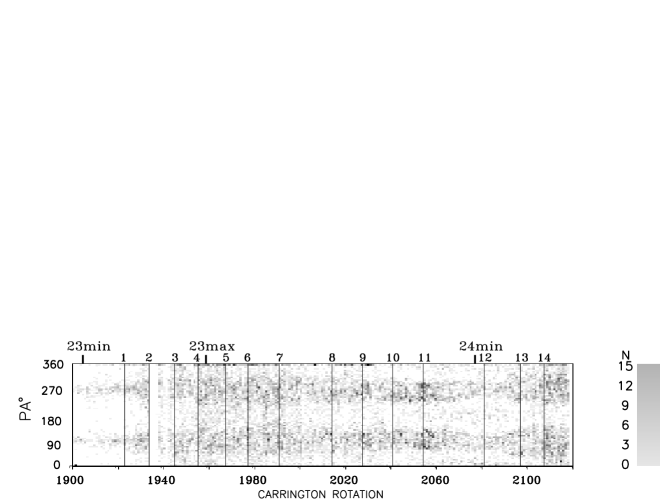
Figure 4.: The PA distribution of CME occurrence rate calculated for each CR in PA increments of $5^{\circ}$ for 1996 - 2011 (CRs 1905 - 2119). Thin vertical lines mark the moments of change in the GMFS.cmelat

From Figure cmeb we can see that there were periods when the CME latitudinal distribution was more uniform (CRs: 1958-1962, 1980, 1993, 2017, 2029, 2042, 2056, 2107). It is seen that points (each point represents an individual CME) show some concentration to the moments marked by these lines, the moments of the GMFS reorganization. To analyze the PA (latitudinal) distribution of CMEs, the occurrence rate was calculated for each CR in PA increments of $5^{\circ}$. In Figure cmelat the distribution for each CR versus PA is shown. In order to evaluate the homogeneity of CME latitudinal distribution, the coefficient of uniformity $K_{u}$ was calculated Frozini (1987) from the distribution in Figure cmelat.

$$K_{u}={\frac{1}{\sqrt{n}}\sum_{i=1}^{n}\Bigl{|}N_{i}-\frac{i-0.5}{n}\Bigr{|}},$$ (4)

where $N_{i}$ is the number of CMEs in each $5^{\circ}$ latitudinal step; $n$ is the number of steps in each CR. Coefficient $K_{u}$ describes the latitudinal uniformity of CME distribution on the solar disc for each CR. Figure globkoefe presents the $K_{u}$ coefficient evolution. To filter out high frequency variations, Ku were smoothed with 3 CRs. The growth in $K_{u}$ means an increase in the inhomogeneity of the latitudinal distribution of CMEs in a CR. With increasing uniformity in the CME latitudinal distribution the $K_{u}$ coefficient decreases. With the solar activity increase the CME distribution over latitude became more uniform. Thin vertical lines in Figure globkoef mark the moments of reconfigurations in the GMFS. The comparison of Figures londiaga, londiagb, and globkoefc and globkoefe shows that the moments of the changes in GMFS (peaks in $K_{lon}$) and $K_{u}$ decrease (which means the increase in the CME latitudinal (PA) homogeneity) marked by vertical lines coincide. This allows us to conclude that the uniformity of CME latitudinal distribution increases when the GMFS changes. In Figure cmelat thin vertical lines, marking the same moments, are shown. However, the coincidence is not completely accurate, because, as can be seen from Figures londiaga, and londiagb the reorganization of the GMFS requires at different longitudes 1-3 CRs. It should be also noted that CMEs are associated with different solar activity phenomena that can respond to the reorganization of the GMFS in different ways and time delay.

In Figure cmehu the dependencies of CR averaged CME rate and parameters on the global magnetic field parameters such as calculated source surface magnetic field strength $|H|$ and magnetic field of the Sun as a star $|H_{s}|$ and $K_{u}$ are summed up. Here, each point represents a CR averaged CME data. All CME data were divided according to the domination of the zonal or sectorial structure of the global magnetic field Bilenko (2012). Light blue indicates CMEs of the minimum of cycle 23, which corresponds to the zonal structure domination (CRs 1905-1930). Blue denotes CMEs of the maximum and the beginning of the decay phase of cycle 23, corresponding to the sector structure of the solar global magnetic field (CRs 1930-2007). Red denotes CMEs of the minimum of cycle 24, and the time of the zonal structure domination (CRs 2007-2087). Green represents the CMEs of the growing phase of cycle 24, and sector structure domination (CRs 2087-2119).

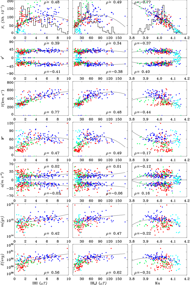
Figure 5.: Interrelations between CME parameters and $|H|$, $|H_{s}|$, and $K_{u}$.cmehu

Thin lines denote a second-order polynomial fit. All dependencies, shown in Figure cmehu are non-linear. Therefore Spearman Spearman (1904) rank correlation coefficient ($\rho$), which is a non-parametric measure of statistical dependence between two series, was calculated.

$$\rho=1-\frac{6\sum\limits_{i=1}^{n}(R_{1i}-R_{2i})^{2}}{n(n^{2}-1)}$$ (5)

where n is the length of time series, $R_{1i}$ and $R_{2i}$ - the ranks of the compared time series. Correlation coefficients are shown in each panel. The significance level for these time series is equal to 0.155. For the most dependencies the correlation found can be of physical significance with the exception of acceleration.

In the first row, the histograms are shown. The dependencies of CME parameters from $|H|$ (the first column) show that they consist of three groups. The first group includes the majority of CMEs of the minimum of cycle 23 and the minimum and rising phases of cycle 24. This group is associated with low magnetic field strength $|H|<3\,\mu T$. The CMEs of the first group are located near the solar equator, they have low speed from $200\,km\,s^{-1}$ to $400\,km\,s^{-1}$, width from $15^{\circ}$ to $90^{\circ}$, low mass, and energy. The acceleration varies widely $\sim\pm 70\,km\,s^{-2}$. The second group is associated with the magnetic field strength from $3\,\mu T$ to $5.5\,\mu T$. CMEs have speeds from $250\,km\,s^{-1}$ to $600\,km\,s^{-1}$, width from $40^{\circ}$ to $90^{\circ}$, they have moderate acceleration, mass, and energy. And the third group is associated with magnetic field strength greater than $5.5\,\mu T$. These CMEs have high speed, acceleration, mass, and energy, but moderate width. The dependencies of CME parameters from $|H_{s}|$ are presented in the second column. They are also consist of several groups and have similar distributions and correlations.

The dependencies of CME parameters from $K_{u}$ are shown in the third column. The histogtam is peaked around $K_{u}=4.03$. It is seen, that the maximum uniformity is achieved when the sector structure of the global magnetic field is dominated (blue and green, $K_{u}$ is low). CMEs associated with the zonal global magnetic field structure distributed less uniformly (light blue and red, $K_{u}$ is high).

Figure 6.: (a) CME position angle; (b) AR projected angle; (c) AR longitude distribution; (d) the longitude distribution of ARs with the area greater than 300 m.v.h.; (e) CME occurrence rate; (f) AR occurrence rate; (g) AR area (m.v.h.); (h) Spot number in each AR. Thin lines, in (e-h), denote CR averaged data and thick lines correspond to 7 CR averaged data. Thin vertical lines mark the moments of change in the GMFS.arlatlon

As a rule, most articles on CMEs consider their relation to the AR local magnetic fields. CMEs occur more commonly where magnetic fields are stronger, more complex and vary more rapidly (Hildner1976). But the size of ARs seems to not play an important role in CME eruptions as sometimes very small ARs are able to produce CMEs Schmieder (2006). The fastest CMEs are known to originate from an instability of AR strong complex magnetic fields with shear and twist (Falconer2002; Gao2011). Figure arlatlon displays the CME rate and PA distribution together with the AR distribution and parameters. Figure arlatlona shows the PA for all CMEs. For comparison with CME distribution, the latitude of each AR were converted to projected angle (Figure arlatlonb). In Figure arlatlonc, the longitudinal distribution of all ARs, and in Figure arlatlond, for those with area greater than 300 millions of visible hemisphere (m.v.h.), are presented. CR averaged CME occurrence rate ($N_{CME}$) is shown in Figure arlatlone. CR averaged AR rate ($N_{AR}$) is shown in Figure arlatlonf, and the CR averaged area of ARs ($S_{AR}$) is shown in Figure arlatlong. The evolution of the number of spots in each AR ($P_{AR}$) is presented in Figure arlatlonh. Thin lines in Figures arlatlone -arlatlonh denote CR averaged data, and thick lines denote 7 CR averaged data. The timing of the changes in the structure of GMFS are marked by thin vertical lines.

From Figures globkoef, cmea, and arlatlone it is seen that the increase in CME number was not smooth and gradual during the rising phases, but it had the form of individual bursts (lines 1, 2, 3, and 13, 14). $K_{lon}$ impulses were rather high, reflecting the reorganizations of the GMFS in a wide range of longitudes. The impulses in $K_{lon}$ coincided with the growth in $K_{c}$ and an increase in AR number and area. The simultaneous increase in AR number and area indicates that a new magnetic fields is formed, in general, by the emergence of a new magnetic flux forming new ARs Ballester, Oliver, and Baudin (1999). The coincidence of CME and AR impulses suggests that the increase in CME activity was associated with ARs at that time.

The latitude distribution of CMEs changes during solar cycles (Hundhausen1984; Hundhausen1993; Yashiro2004; Lara2005; Lara2008; Robbrecht2009a). Hundhausen1993 noted that in the beginning of a solar cycle the latitude distribution of CMEs and ARs is different. The ARs of a new cycle emerged at latitudes about $\pm 30^{\circ}$, and CMEs are concentrated to the equator. But at the beginning of cycle 24 CMEs were widely spread over the solar latitude.

From Figures arlatlone and arlatlonf it can be inferred that just like the AR, the CME occurrence rate rose during the growing phase and decayed after solar maximum. The decay was not a smooth exponentially decaying process, but it had a number of peaks that were comparable in magnitude to the values of CME parameters at the maximum of cycle 23. In Figures cmeb, arlatlona the general latitudinal drift of low-latitude CMEs towards the equator during the declining phase is clearly distinguished. It most likely reflects the changes in the latitudinal distribution of the CMEs associated with ARs. But the decay rate of CMEs was lower than that of ARs. Robbrecht2009a have proposed that some CMEs originated from non-sunspot regions at that time. According to Obridko2012 the CMEs can be associated with the giant cells and coronal holes.

It is well known that there are two peaks in Wolf number separated by Gnevychev gap (the dip in the solar activity). Secondary solar activity peak occurred two to three years after the main maximum (Gnevyshev1963, 1967). In cycle 23 the first peak was in April 2000 (CR 1962, $W=120.8$) and the second peak occurred in November 2001 (CR 1983, $W=115.5$). CME rate, Figures cmea and arlatlone, also shows two peaks and the gap. The gap in CME evolution was also retrieved in the CACTus data Robbrecht, Berghmans, and Van der Linden (2009). According to Robbrecht2009a and Ramesh2010, the CME second peak shows a delay of 6 to 12 months with respect to the sunspot index. Our result shows the delay for the second peak was equal to 10 CRs.

From Figures cme and arlatlon we can see that during each peak, the growth of CME and AR number was in the form of individual impulses. But the rate of CMEs closely followed the ARs only during the rising phase and the first peak. They were differed greatly during the second peak and the declining phase. Comparison with Figure londiag shows that the first peak occurred when the large two-sector structure appeared. From Figures londiaga and londiagb, it is seen that the Gnevychev gap coincides with the change in GMFS and the periods of oscillations. The periods of $\sim 40\div 80$ d and $\sim 100\div 200$ d weakened and disappeared and the periods of of $\sim 40\div 80$ appeared. A quasi-stable two-sector structure existed from CR 1970 to CR 1980 (lines 5, 6). The structure coincided with the gap in CME rate. The number of CMEs diminished, they had on average higher velocity, lower acceleration and rather narrow width. Since CR 1980 (line 6) the periodicities with periods of $\sim 50\div 100$ d appeared again, the periods of $\sim 100\div 200$ d began to grow and the GMFS reversed the polarity. The CME second peak (line 7, CR 1993) coincided with the changes in GMFS at longitudes $90^{\circ}-180^{\circ}$ with the disappearance of periods of $\sim 150\div 200$ d and appearance of periods $\sim 100\div 120$ d and $\sim 40\div 80$ d. There was no large new magnetic flux emergence ($K_{c}\sim 0.1$). The uniformity of CME latitudinal distribution was very high. The rate of CMEs during the second peak was higher than that during the first peak. The scale of the rearrangement of the GMFS was practically the same. Moreover, the positive-polarity and negative-polarity magnetic fields of the new structure appeared at the same longitudes as those of the structure existing at the time of the first peak, and the periods of oscillations were the same. The GMFS reorganization during the second CME peak covered a larger longitudinal interval compared to the first one ($K_{lon}$ was equal to $\sim$0.5). The magnetic field strength was also higher. The uniformity of CME latitudinal distribution increased (Figure londiage). In the longitudinal distribution of ARs (Figure arlatlonc, arlatlond) it is seen that the majority of ARs were observed from CR 1940 to 2000, when the long-lived two-sector structures with a high magnetic field strength were existing. The comparison of CME and AR PA distributions, Figure arlatlona and arlatlonb, shows that they are similar for CME population concentrated to the AR latitudes. But equatorial CMEs spread over a much wider region than ARs. Some of such CMEs can be the result of eruption of cross-equatorial arcs connecting ARs located in the North and in the South hemispheres Lara (2008). Some CME source regions may be close to one of the ARs from cross-equatorial arcs and suffer a strong deflection toward the equator Lara (2008). Some high-latitude CMEs could be the projections of processes at the latitudes of ARs, or may be the result of non-radial propagation of erupted filaments caused by the global magnetic field configuration Filippov, Gopalswamy, and Lozhechkin (2002).

During the declining phase, the sharp extensions in AR area were seen in Figure arlatlong. But the number of ARs did not increase. According to Ballester1999, if the increase in the area of AR is not accompanied by an increase in the number of ARs, it means, that there is a new magnetic flux emerging in already existing ARs. In Figure arlatlonh the increase in spot numbers in each AR, coinciding with the AR area impulses, is observed. Therefore, the complexity of ARs increased. Such ARs are known to be the sources of flares and, obviously, eruptive events. This may explains the increase in high velocity CMEs during the decay phase. High velocity, narrow CMEs with high acceleration were probably the consequence of the processes occurring in ARs (CME parameters between the lines 8-11). The comparison of Figures cme and arlatlon shows that the oscillations in CME parameters, observed during the declining phase, were the result of the alternation of two processes. The first one was the emergence of a new magnetic flux coinciding with the AR area and it’s complicity growth. The CMEs associated with that process (between vertical lines 8-11) had, on average, higher velocity, lower width and higher acceleration. The flux emergence in ARs could be the source of solar flares. CMEs associated with flares have higher V. The second process was associated with the GMFS reorganizations. The CMEs associated with the GMFS reorganization, marked by vertical lines (8-11), were characterized by low velocity, low acceleration, yet higher width.

Figure 7.: (a) dashed line the number of CMEs with $V>600\,km\,s^{-1}$ and solid line those with $V\leq 600\,km\,s^{-1}$; (b) dashed line the number of CMEs with $W>50^{\circ}$ and solid line those with $W\leq 50^{\circ}$; (c) dashed line the number of CMEs with $a>\pm 20\,m\,s^{-2}$ and solid line those with $a\leq\pm 20\,m\,s^{-2}$; (d) dashed line the number of CMEs with $m>1.710^{15}\,g$ and solid line those with $m\leq 1.710^{15}\,g$; (e) dashed line the number of CMEs with $e>2.10^{30}\,erg$ and solid line those with $e\leq 2.10^{30}\,erg$. thin lines the difference between the number of CMEs with lower and higher than a corresponding limit for each parameter. Thin vertical lines mark the moments of change in the GMFS.cmeparam

As has been shown above, the number of CMEs during the CRs of the GMFS reorganization increased and the parameters of the CMEs were different from those during the periods of quasi-stable GMFS. In Figure cmeparam the number of CMEs, depending on their parameters, is shown. The changes in the structure of the GMFS are marked by thin vertical lines.

At the times of the GMFS reorganizations, market by vertical lines, the relative number of weak, low-speed, low-accelerated CMEs with low mass and energy, increase greatly compared to power events, except the lines 1, 2, 5, and 12. Line 1 corresponds to the beginning of cycle 23. At that time, no significant events were observed. Line 5 corresponds to the maximum of cycle 23. But, during solar maxima the number of small, faint events is underestimated due to the occulting effect of power CMEs. Line 12 corresponds to the deep minimum of activity, when there are very few events related to the CMEs. The difference (thin lines) in the number of CMEs with parameters lower the limits and that greater the limits increased during the GMFS reorganizations. It suggests that, in general, fast variations in GMFS make the conditions favorable for weak, low-mass, low-energy highly accelerated CMEs. The number of CMEs with $V>600$ shows local increases between the lines (between the GMFS reorganizations). The number of CMEs with the width greater than $50^{\circ}$ and that of CMEs with the width less than $50^{\circ}$ was almost the same during the maximum. The decrease in both of them coincided with the Gnevishev gap and they peaked when large-scale structures were existing. But they were very different in the decay phase. The number of CMEs with $W<50^{\circ}$ and the difference between the number of CMEs $W<50^{\circ}$ and that $W>50^{\circ}$ increased greatly at the moments of the GMFS reorganizations during the decay phase (line 11).

5 On the possible relation of Rossby waves and CMEs

secrosbywave

Gilman proposed that observed solar magnetic fields can be the result of Rossby waves generated around the thin magnetized layer at the bottom of the convection zone (Gilman1969a; 1969a; 1999). Rossby waves belong to a subset of global waves that can exist in a fluid layer on the surface of a rotating sphere. On the Sun Rossby waves are strong during the maxima phases and have periods greater than solar sideral rotation period (Lou2000; Zaqarashvili2010a; Zaqarashvili2010b). In Tikhomolov (1995, 1996) Rossby vortices were considered to explain the observed GMFS. It was proposed that Rossby vortices were excited within a thin layer beneath the convection zone. They are a result of heating from the solar interior and the deformation of the convection zone lower boundary. According to Zaqarashvili et al., (2010a, 2010b) the periodicity of 155-160 days and $\sim$2 years, observed in different solar activity indices, can be connected to the dynamics of magnetic Rossby waves in the solar tachocline, since in the layer they are unstable due to the joint effect of the toroidal magnetic field strength and latitudinal differential rotation. It was also proposed that equatorially trapped Rossby-type waves might modulate solar flares, ARs Lou (2000) and CME Lou et al. (2003) activity. But in GALLEX (GALLium Experiment) data the periodicities of 52 d, 78, d and 154 d were also revealed (Sturrock1997; 1999). The analysis has shown that the solar neutrino flux exhibits a periodic variation that may be attributed to rotational modulation occurring deep in the solar interior, either in the tachocline or in the radiative zone Sturrock, Walther, and Wheatland (1997). These periodicities probably result from Rossby-type waves occurring in the solar interior. It means that Rossby waves are generated deep in the solar interior such as the base of the convection zone, rather than at the photosphere. In Kuhn et al. 2000 the observation evidence, confirming the existence of Rossby waves in the photospheric magnetic field, using observations of the Michelson Doppler Imager (SOHO), is presented.

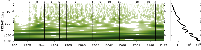
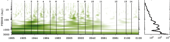
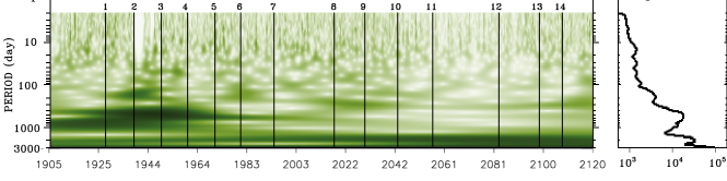
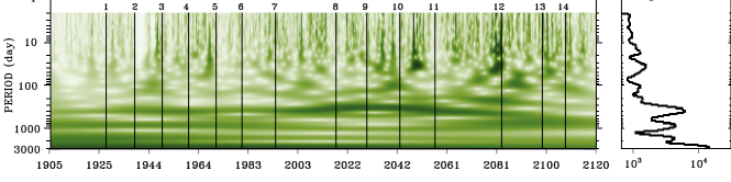
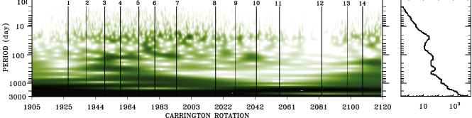
Figure 8.: The wavelet power spectra of (a) CME daily rate; (b) CME velocity; (c) CME angular width; (d) CME positive acceleration; (e) AR. Thin vertical lines mark the moments of change in the GMFS.cmewave

Figure 9.: (a) and (b) periods from the wavelet decomposition of MF. (c) and (d) periods from the wavelet decomposition of CME number. In (a) and (c) solid line P=50-70d; dash dot line P=90-100d; long dashes P=100-120d. In (b) and (d) solid line P=200-220d; dash dot line P=300-400d; long dashes P=600-700d. Thin vertical lines mark the moments of change in the GMFS.waveper

From Figure cme it is seen that the oscillations in CME rate and parameters did not coincide for different CME parameters and were different at different solar cycle phases. The strongest oscillations were observed during the decay phase. The amplitude of oscillations was about $400\,km\,s^{-1}$ for individual CME velocity and $\sim 200\,km\,s^{-1}$ for 7 CR averaged data (Figure cme). The intense spike (CR 2009) in the CR averaged CME velocity and width was due to the Halloween 2003 storm Gopalswamy (2005). The oscillations were most pronounced in the CME acceleration. The positive and negative accelerated CMEs had almost the same amplitudes and they varied synchronously (Figure cmee). The CME parameters and daily rates have been analyzed using a Morlet wavelet technique to look for the presence of the periods and the temporal evolution of these periods (Figures cmewavea-d) and Figure waveper). Wavelet power spectrum of AR daily rate is also shown in Figure cmewavee. Wavelet spectra for periods greater than $\sim 3000$ d are not reliable, as these periods are not much less than the total data length of 5475 d (edge effects). The strong peaks around $\sim 27$ d were defined in the MMF (Figure londiagc) and in AR spectra, but they do not present neither in CME rate nor in CME parameter wavelet spectra (Figure cmewavea-d). The first peak was around $\sim 30-40$ d in CME spectra. In CME wavelet spectra periods greater than 100 d dominate. Periods of $300\div 400$ d were present in MMF and in CME. They were absent in AR since CR 2017. There is also a match around a periodicity of $\sim 100-150$ d in both MMF and CME during CRs 1993 - 2017 (lines 7-8). These periodicities were also not present in AR. MMF and CME have also comparable lowering frequency oscillations from CR 2017 to CR 2056. This may be interpreted as large-scale magnetic field driven periodicities in CME data. It can be seen that there is a temporal coincidence between the periods corresponding to MMF and CME spectra and again when the periodicity appeared/disappeared in MMF they also appeared/disappeared in CME (Figures cmewavea-d) and Figure waveper). Comparison of Figure cme with Figure londiag and cmewave shows that the peaks in CME number coincided with the formation of new periods and the GMFS reorganizations. This comparison makes a strong case for a relationship between the appearance of the periodicity in CMEs and the changes in the GMFS. A time and frequency coincidence between both periodicities suggests the existence of a casual link between them. The time coincidence in the waves appearing/disappearing is thought to be very important and seems to confirm the existence of a casual link between them. Some periods in CME spectrum are associated with ARs, especially during the maxima of cycle 23. The periods of $50\div 100$ d coincided in CME and AR from CR 1970 to CR 1993. The fluctuations in CME rate and velocity during the maximum and the declining phase of cycle 23 were also noticed by Ivanov and Obridko Ivanov and Obridko (2001), Lou et al. Lou et al. (2003), Gerontidou et al. Gerontidou et al. (2010). In Lou2003 it was proposed that oscillations with periods 51, 76, 128, and 153 days in CME daily rate would be consistent with the presence of large-scale equatorially trapped Rossby-type waves.

At the beginning of cycle 23, since CR 1949 (line 3) a long-lived two-sector structure with high magnetic field strength was created. The structure was the result of the large amount of a new magnetic flux emergence in a wide longitudinal range (Figures globkoefc, globkoefd). This could be a consequence of the appearance of the oscillation within the period from 100 d to 200 d (Figures londiagc, cmewave). The changes of the periods resulted in the changes in the GMFS and in CME rate growth. Between CRs 1949 - 1959 (between lines 3 and 4) a short-lived unstable structure appeared at longitudes $\sim 120^{\circ}-250^{\circ}$ and, simultaneously, the oscillations with period of $\sim 50-90$ d was observed. The configuration of the GMFS changed from a two-sector to a four-sector and the rate of CMEs diminished. The CMEs associated with that short-lived four-sector structure were, on average, wide and had low acceleration (Figure cme).

Lines 8 - 11 (CRs 2017, 2029, 2042, 2056) were associated with impulses in $K_{lon}$ (GMFS reorganization), but $K_{c}$ (new magnetic field emergence) was low. From, the line 8 four-sector structure was formed and large-scale drifting structures were observed. The step-like decrease in the wave periods was observed in MMF and CME (Figure londiagc, cmewave). The decrease was in the form of separate steps and transition to the each next step was accompanied by the increase in CME number with low speed, width and acceleration. Line 8 (CR 2017) also corresponds to the appearance of a new GMFS at longitudes $0^{\circ}-80^{\circ}$. GMFS changes were not accompanied by a substantial new magnetic flux emergence. The strength of the magnetic field was also low. Since line 9 (CR 2029) the two-sector structure became the four-sector one. The rate of CMEs increased at that moment. On average, the CMEs were faint. During CRs 2035-2045 (line 10) the two-sector structure was restored for a short time. That moment was also characterized by an increase in CMEs with low parameters. The sharp decrease in the rate of CMEs since 2003 ($\sim$ CR 2000) coincided with the decrease of the sector structure contribution Bilenko (2012). A significant reduction in CME number was also observed from that time. On average, the CMEs associated with those periodicities had low speed and acceleration, but they were rather wide.

Since CR 2056 (line 11) the waves at the range from $\sim 40\div 300$ d disappeared (Figure londiagc). The GMFS changed from four-sector to two-sector. Magnetic fields changed their polarity from positive to negative in the longitudes $180^{\circ}-330^{\circ}$ during one CR. But, as it happened during the decay phase, there were no large powerful ARs at that time (Figure arlatlon). There were only very weak new magnetic flux emergence impulses (Figure globkoefd). The intensity of the magnetic field was also low. The rate of CMEs was equal to that of the solar maximum peaks, but the CMEs were faint. They had low speed, small width and low acceleration. Figure globkoefe shows that the uniformity of CME latitude distribution increased greatly at that time.

6 Discussion

secdiscus

According to the previous studies for cycles 21, 22, and 23, CMEs are concentrated to the solar equator in the range $\pm 30^{\circ}$ during solar minima, and their distribution is almost normal. This is consistent with our findings for cycle 23, however, the behavior of CMEs at the minimum of cycle 24 was very different. They were observed at all latitudes. The difference in CME latitudinal distribution may be explained if we take into consideration the difference of the GMFS in the minima of cycles 23 and 24. Near cycle 23 minimum, CRs 1900 - 1930, the coronal field was dipolar, the magnetic field strength was low (Figure globkoefa), the HCS was flat and was located near the solar equator $\sim\pm 25^{\circ}$, the GMFS was fragmented and sharply changed (Figures londiaga, londiagb). But during the minimum of cycle 24, the large-scale two-sector GMFS existed. Sector structure with large-scale interchanging positive-polarity and negative-polarity magnetic fields extending to latitudes of $\pm 40^{\circ}$ on the both sides of the heliomagnetic equator was observed. CMEs are known to be related to the heliomagnetic equator and identified with a belt of coronal helmet streamers (Kahler1987; Hundhausen1984; Hundhausen1993; Mendoza1993). Arcs, connecting opposite-polarity magnetic fields, separated by the HCS, can be the sources of some CMEs. Because the HCS was extended to high latitudes, the CMEs associated with the arcs, were also observed at higher latitudes than that at the minimum of cycle 23. Such CMEs were faint CMEs. They had, on average, low speed, width and mass, but rather high acceleration (Figure cme). Furthermore, the filaments/prominences are known to locate above the magnetic polarity inversion line, hence the eruptions of filaments/prominences will also occur more frequently at higher latitudes.

Figure cmea shows that the occurrence rate of CMEs were higher during the minimum of cycle 24 than that during the minimum of cycle 23. The daily rate of CMEs was $\sim 3-6$ events at the minimum of cycle 24 and only $\sim 2-3$ events at the minimum of cycle 23. A sharp increase in the number of CMEs and their parameters was observed at the beginning of cycles 23 and 24. The daily CME rate rose faster at the beginning of cycle 24 than that of cycle 23 (Figures cmea, arlatlone). For cycle 23, using CACTus CME catalog, Robbrecht2009a found that the daily CME rate, averaged per year, increased roughly with a factor of 4 from the solar minimum to maximum, approximately from 2 events during the minimum, to 8 events during the maximum. In Petrie 2013 based on three independent solar eruption automated catalogs (not CDAW) CACTus (Computer Aided CME Tracking project), SEEDS (Solar Eruptive Event Detection System) and Nobeyama Radioheliograph prominence eruption data, it has been shown that CME rates and prominence eruptions are both higher for years 2003-2012 than for 1997-2002. It was concluded that the result is connected with the weakness of the late cycle 23 polar field and such an increase was explained by the influence of the polar field weakening in the late cycle 23 and the beginning of cycle 24 on the global coronal field structure. Vourlidas et al. 2010; 2011 showed that the CME mass and mass density in 2009 were close to their 1996 values but the kinetic energy was a factor of 1.8 lower and CME velocities were 32% less than in 1996. Robbrecht2009a compared two catalogs CACTus and CDAW. In Figure 3 of that article it is shown that the percentage of narrow CMEs (with the width smaller than $20^{\circ}$), compared to the total number of CMEs, increases in both the CACTus (red) and CDAW (blue) data. Thus, these investigations, using independent data catalogues and methods, provide additional evidence for the increase in CME numbers and especially in small, faint events. CME velocities (Figure cmec) increased for individual CMEs, however, when averaged over CR the growth was not so noticeable. It means that low-velocity CMEs were dominated at the beginning of cycle 24. From Figure cmed it is seen that CME widths have also increased but at the beginning of cycle 24 it increased much slower than at the beginning of cycle 23, and the averaged values were also lower. It means that the majority of CMEs were narrow-width CMEs at the beginning of cycle 24. The average acceleration of CMEs (Figure cmee) changed little from the minimum to the maximum in cycle 23, and it even diminished in cycle 24.

The increase in CME number may have several explanations. SOHO/LASCO have observed more narrow CMEs since 2003 by improving the sensitivity of the instruments. Except that, after 2006, faint CMEs become easier to identify as overall activity decreases Wang and Colaninno (2014). An increase in LASCO telemetry in 2010 resulted in increase of C2 recorded images from 60 to 104 per day, and consequently in increase in the detected CMEs Wang and Colaninno (2014). But in their detailed study based on CME mass estimates it was shown that cycle 24 is not only producing fewer CMEs than cycle 23, but that these CMEs tend to be slower and less massive than those of cycle 23.

It should be noted that in Petrie 2013 not only CME data from the LASCO catalogs were used, but also the Nobeyama Radioheliograph prominence eruption data were analyzed, which are not associated with the changes of LASCO modes and methods. The study showed that the number of faint CMEs increased.

Using ARTEMIS-II, CDAW, SEEDS, and CACTus catalogs, Lamy et al. (2014) found that all four catalogs agree on the fact that the CME rate has been increasing faster than the activity index (SSN and F10.7) during the rising phase of solar cycle 24. They found also that the difference between the cycles 23 and 24 minima is conspicuous and characterized by a broader and fainter equatorial belt in cycle 24 Lamy et al. (2014).

Hudson et al. (2014) studding the annual averages of active region flare productivity, on the base of NOAA ”events” database, have found that ARs in 2004-2005 (CRs 2012-2038) had flare productivity about twice as large as those at other times. This increase coincide with the peaks in CME number and GMFS changes (lines 8, 9). It means that some of these CMEs are the result of that flares. They noted also that the RHESSI flare counts show an increase in flare productivity at the C-class level, beginning from October 2003 Hudson, Fletcher, and McTiernan (2014). According to Hudson and Li (2010), the flare/CME ratio diminished by almost an order of magnitude in the cycle 24 minimum. They suggest that the cycle 24 minimum corona was relatively easy to disrupt. It was also found that the global radiance of the K corona was 24% fainter during the minimum of solar cycle 24 than during the minimum of solar cycle 23 Lamy et al. (2014).

Thus, the increase in the number of weak CMEs is determined not only by changing of the monitoring regime and CME detection method, but also by a real increase in the weak events that are the result of the reducing of the solar global magnetic field strength.

According to our results, CMEs do not effect the GMFS to a great degree. Some changes were observed in the border of the structure only. There were a lot of CMEs during the maximum and the beginning of the decline phase of cycle 23, but the total GMFS remained quasi-stable during the rather long time of $\sim 1-5$ years. There were 2 large GMFS reorganizations only (in CRs 1970 and 1980) leading to the global redistribution of the positive-polarity and negative-polarity magnetic fields. Moreover, during the reorganizations the number of weak, low-energy CMEs increased (Figure cmeparam). Therefore, CMEs are the consequence of the GMFS reorganization and not the cause. In Lio (Figure 2 in Liu2009) it is observed, as described in the article, that the CME event caused the local changes in the shape of the border of the GMFS. But we can see that the general distribution of positive-polarity and negative-polarity magnetic fields remained unchanged. Some small short-lived changes in the GMFS may be caused by some powerful CMEs. Such changes in the GMFS shape observed during the declining phase, visible in Figure londiaga, londiaga, CRs $\sim 2034\div 2082$ d, as extensions from the main large-scale structure, may be the results of some CMEs. But these changes are short in time $\sim 1-3$ CRs. CMEs can have influence on the shape of the GMFS and change the local shape of the structure only. They do not change the total distribution of magnetic fields.

It is interesting to note, that during the declining phase, when the oscillations in CME parameters are more pronounced, the increase in CME number coincide with the decrease in AR parameters, such as area, extension and the number of spots in each AR (Figure arlatlon). The timing of the GMFS reorganizations are marked by thin vertical lines. The strength of the magnetic field diminished during these times (Figuresglobkoefa, globkoefa). AR parameters increase between vertical lines, i.e. between the moments of the GMFS reorganizations. But CME number increases in times marked by vertical lines (the times of the GMFS reorganizations). It means that at least CMEs associated with that ARs are not the cause of the GMFS reorganizations.

The GMFS is not the cause of CMEs itself, but the structure of the global magnetic field determines the conditions favorable for CMEs. Nevertheless, all the CMEs are caused by loss of equilibrium of the pre-existing magnetic structure. When the GMFS changes the magnetic field strength both of the magnetic field calculated at source surface and that measured on the Sun as a star diminished (Figures globkoefa, globkoef2b). But the strength of the external magnetic field is known to play an important stabilizing effect on CME eruptions Schmieder (2006). Even small instability may lead to an eruption and CMEs became more frequent when the magnetic ”frame” is disrupted. But these CMEs are faint CMEs. There is no time to accumulate large energy because even a small instability can cause an eruption. They do not need to be energetic event to disrupt the overlying magnetic field structure. The strength of the global magnetic field is low. When GMFS remains quasi-stable during a long time period, large long-lived ARs and filaments/prominences can be formed and large amounts of energy can be accumulated, which is need to disrupt the existing magnetic configuration in the solar corona, because the magnetic field of the global magnetic field is high. At the solar cycle maximum, large long-lived two-sector magnetic structures were observed. The more stable and larger the structure and higher the magnetic field strength, the larger and more complex the ARs that can be formed. Large, long-lived ARs of complex magnetic field produce intense CMEs. During the solar activity maximum the increase in CME acceleration was accompanied by increases in velocity, width, mass and energy. The evolution of the global magnetic field, both the magnetic field strength and GMFS, controls the general situation in the Sun’s atmosphere as well as directs the conditions for CME occurrence rate and parameters.

The large structures and redistributions of the GMFS during the cycle 23 maxima and the beginning of the declining phase coincide with two peaks in ARs and CMEs activity. It seems that the second CME peak was developed independently from the AR second peak, and at the same longitudes and with the same distribution of GMFS as the first CME peak. According to Robbrecht2009a and Ramesh2010 the CME second peak shows a delay of 6 to 12 months with respect to the sunspot index. Our result shows the delay for the second peak was equal to 10 CRs. Robbrecht2009a have proposed that the observed time delay gives an idea of the time needed to build up the necessary conditions for CME activity. According to Du2012, a double peak suggests that there are two sources or two decay time scales. The presence of two peaks may indicate the existence of two waves of activity, each related to one another, but differing appreciably in their characteristics Antalova and Gnevyshev (1965). In Benevolenskaya, (1998, 2003), the double peak-structure of the AR solar cycle was explained as a consequence of the impulsive nature of the solar activity, or a manifestation of the double magnetic cycle of two dynamo sources separated in space. It was proposed that a low-frequency component is generated at the bottom of the convection zone and produces the 22 year magnetic cycle. The impulses of solar activity with the period of $1.5-2.5$ years are formed near the top of the convection zone by reappearing long-lived complexes of activity, and that these impulses can be explained by the high-frequency component of the toroidal magnetic field. The hypothesis of time-space organization of sunspot activity, like impulses, was considered in Gnevyshev (1963, 1966, 1967, 1977), Zolotova2012. Therefore, the two-peak structure is a result of the global magnetic cycle evolution.

The observed periodicities in CMEs could be attributed to a Rossby-type-wave induced variation of the solar global magnetic field. We suggest that GMFS and the GMFS reorganizations, as described above, are a consequence of the changes in the source of excitation of Rossby waves of different periods in the solar tachocline. It is proposed that the reconfigurations of the GMFS are associated with the Rossby wave period changes. Each change in the oscillation period is associated with the GMFS change, which result in the destruction of the existing coronal magnetic structure, and consequently, in the increase in the number of CMEs and in the changes of their parameter. Therefore, the CMEs of the time of the quasi-stable GMFS and that of the time of the changes in wave periods and consequently the reorganization of the GMFS, have, on average, different parameters.

Thus, the changes in the wave periods and structural reorganizations in the global magnetic field can result in the formation of weak CMEs. This may be the explanation of the formation of CMEs that are not accompanied by any solar activity phenomena (flares, filament eruptions, arcs, etc.), for example, such as, the CME event observed on 2008 June 2 and described in Robbrecht2009b. The event originated along a neutral line over the quiet Sun. There were no any ARs. The CME was wide and had low speed ($<300\,km\,s^{-1}$). The photospheric fields were weak ($<3G$). The event was classified as streamer-blowout CME. The probable source region of the CME was from $30^{\circ}$ to $100^{\circ}$ in CR longitude. According to our investigation, these features are the characteristic of a CME associated with GMFS reorganization. From Figure londiag we can see that there was an abrupt change in the shape of the large two-sector structure in the longitudinal range $0^{\circ}\div 100^{\circ}$ at that time (CR 2071). The changes could lead to instability in the solar corona and CME. Ma2010 have found that the velocities of the CMEs without distinct low corona signatures generally range between $100\,km\,s^{-1}$ and $300\,km\,s^{-1}$. They noticed that some faint changes of the coronal structures could be observed over the solar limb during such a CME.

7 Conclusion

seccon

The detailed comparison of CME and GMFS cycle evolution shows that CME activity is not chaotic but it is regulated by evolutionary changes in the solar global magnetic field. The evolution of the global magnetic field, both the magnetic field strength and GMFS, control the general situation in the Sun’s atmosphere and direct the conditions for CME occurrence rate and parameters. The likelihood of a CME increases rapidly at the moments of GMFS reorganizations. CMEs do not greatly effect the large-scale long-lived GMFS. Only some changes in the border of the structure can be caused by a CME. There is a good relationship between CR averaged CME number, position angle, speeds, width, mass, and energy and global magnetic field strength. Spearman correlation coefficients are 0.48, 0.40, 0.77, 0.47, 0.42, 0.56 respectively (the significance level is equal to 0.155).

CME activity has an impulse-like character. During the rising phases of cycles 23 and 24 the impulses in CMEs coincided with the impulses in AR and their area. They also coincided with the reorganizations of the GMFS in a wide range of longitudes, and with the growth in the new flux emerging. New magnetic fields are formed, in general, by the emergence of a new magnetic flux forming new ARs. The coincidence of CME and AR impulses suggests that the increase in CME activity was associated with ARs. During the declining phase a new magnetic flux emerged in already existing ARs. The oscillations in CME parameters, observed during the declining phase, were the result of the alternation of two processes. The first one was the emergence of a new magnetic flux coinciding with the AR area and complicity increase. The CMEs associated with that process had, on average, higher velocity, lower width and higher acceleration. The second process was the structural change in the global magnetic field. The CMEs associated with the GMFS reorganization were characterized by low velocity, low acceleration, but higher width. The rate of CMEs exceeded that of ARs indicating that CMEs were associated with some other phenomena such as streamers, arcs or filament/prominence eruptions not associated with ARs. Because the HCS was extended to the high latitudes during the declining phase of the cycle 23, the CMEs were also located at higher latitudes.

Our result shows the delay for the second CME peak relative to the second AR peak was equal to 10 CRs. During each peak, the growth in CME and AR rate was in the form of individual impulses. The rate of CMEs closely followed that of ARs only during the rising phase and the first peak, however, they were very different during the second peak. The second CME peak was higher than the first one. Moreover, the new GMFS, associated with the second peak, appeared in the same longitudes as those of the structure existing at the time of the first peak, and the periods of oscillations were the same. The GMFS reorganization during the second CME peak covered a larger longitudinal interval compared to the first one.

It is suggested that Rossby waves generated in the solar tachocline result in the observed GMFS. The changes in the periods of the magnetic Rossby waves result in the reorganizations of the GMFS which lead to the destruction of the existing coronal magnetic field structure and consequently the increase of faint CMEs at the right range of latitudes. The periods of Rossby waves that can be associated with the GMFS lie in the range $\sim 50\div 1000$ d. The wave periods became shorter from $\sim 400\div 50$ d from the minimum to the maximum of cycle 23, and they grew to the minimum of cycle 24 again. The process was not a smooth one, but it had a form of individual steps. Each period remained quasi-constant until a new one appeared. The observed GMFS seems to be a consequence of the excitation of Rossby waves of different periods. Each Rossby wave period favors a particular GMFS. The changes in wave periods coincide with the GMFS reorganization and in the CME location, occurrence rate and parameter changes. The CME rate and parameters depend on the sharpness of the GMFS changes, the strength of the global magnetic field and the phase of a cycle.

These results are important for understanding the global magnetic field evolution over a solar cycle as well as the complete picture of CME occurrence rate and parameter changes. Further investigative research is required to uncover the physical mechanisms behind the wave generation, and consequently the GMFS formation and reconfiguration and its influence on CMEs. This research is of great importance, especially in the context of solar-terrestrial interaction.

Acknowledgements

This CME catalog is generated and maintained at the CDAW Data Center by NASA and The Catholic University of America in cooperation with the Naval Research Laboratory. SOHO is a project of international cooperation between ESA and NASA.

Wilcox Solar Observatory data used in this study was obtained via the web site $http://wso.stanford.edu\,at\,2013:10:19\,06:34:02$ PDT courtesy of J.T. Hoeksema. The Wilcox Solar Observatory is currently supported by NASA.

Information from the Space Weather Prediction Center, Boulder, CO, National Oceanic and Atmospheric Administration (NOAA), US Dept. of Commerce were used.

References

- Alexander et al. (1996) Alexander, D., Harvey, K.L., Hudson, H.S., Hoeksema, J.T., Zhao, X.: 1996, In: AIP Conf. Proc. Solar Wind Eight, Amer. Inst. of Phys., New York, v. 382. ed. Winterhalter, D. et al., 84.
- Altschuler and Newkirk (1969) Altschuler, M.D., Newkirk, G.: 1969, Solar Phys. 9, 131. doi:10.1007/BF00145734.
- Altschuler et al. (1975) Altschuler, M.D., Trotter, D.E., Newkirk, G.J., Howard, R.: 1975, Solar Phys. 41, 225. doi:10.1007/BF00152968.
- Altschuler et al. (1977) Altschuler, M.D., Levine, R.H., Stix, M., Harvey, J.: 1977, Solar Phys. 51, 345. doi:10.1007/BF00216372.
- Antalova and Gnevyshev (1965) Antalova, A., Gnevyshev, M.N.: 1965, Sov. Astronomy 9, 198.
- Bai (1990) Bai, T.: 1990, Astrophys. J. 364, L17. doi:10.1086/185864.
- Ballester, Oliver, and Baudin (1999) Ballester, J.L., Oliver, R., Baudin, F.: 1999, Astrophys. J. 522, L153.
- Bemporad et al. (2005) Bemporad, A., Sterling, A.S., Moore, R.L., Poletto, G.: 2005, Astrophys. J. 635, L189. doi:10.1086/499625.
- Benevolenskaya (1998) Benevolenskaya, E.E.: 1998, Astrophys. J. 509, L49.
- Benevolenskaya (2003) Benevolenskaya, E.E.: 2003, Solar Phys. 216, 325.
- Bilenko (2004) Bilenko, I.A.: 2004, Solar Phys. 221, 261. doi:10.1023/B:SOLA.0000035067.88819.40.
- Bilenko (2009) Bilenko, I.A.: 2009, Geomagnetism and Aeronomy 49, 1114.
- Bilenko (2012) Bilenko, I.A.: 2012, Geomagnetism and Aeronomy 52, 1005.
- Bravo, Blanco-Cano, and Nikiforova (1998) Bravo, S., Blanco-Cano, X., Nikiforova, E.: 1998, Solar Phys. 180, 461.
- Brueckner et al. (1995) Brueckner, G.E., Howard, R.A., Koomen, M.J., Korendyke, C.M., Michels, D.J., Moses, J.D., Socker, D.G., Dere, P.L. K. P.and Lamy, Llebaria, A., Bout, M.V., Schwenn, R., Simnett, G.M., Bedford, D.K., Eyles, C.J.: 1995, Solar Phys. 162, 357. doi:10.1007/BF00733434.
- Bumba and Howard (1969) Bumba, V., Howard, R.: 1969, Solar Phys. 7, 28. doi:10.1007/BF00148402.
- Chen and Shibata (2000) Chen, P.F., Shibata, K.: 2000, Astrophys. J. 545, 524. doi:10.1086/317803.
- Choudhary et al. (2014) Choudhary, D.P., Lawrence, J.K., Norris, M., Cadavid, A.C.: 2014, Solar Phys. 289, 649 656. doi:10.1007/s11207-013-0392-7.
- Cremades and Cyr (2007) Cremades, H., Cyr, O.C.S.: 2007, Adv. Space Res. 40, 1042. doi:10.1016/j.asr.2007.01.088.
- Du (2012) Du, Z.L.: 2012, Solar Phys. 278, 203. doi:10.1007/s11207-011-9925-0.
- Fainshtein and Ivanov (2010) Fainshtein, V.G., Ivanov, E.V.: 2010, Sun and Geosphere 5, 28.
- Falconer, Moore, and Gary (2002) Falconer, D.A., Moore, R.L., Gary, G.A.: 2002, Astrophys. J. 569, 1016. doi:10.1086/339161.
- Filippov, Gopalswamy, and Lozhechkin (2002) Filippov, B.P., Gopalswamy, N., Lozhechkin, A.V.: 2002, Astronomy Reports 46, 417.
- Floyd, Lamy, and Llebaria (2014) Floyd, O., Lamy, P., Llebaria, A.: 2014, Solar Phys. 289, 1313. doi:10.1007/s11207-013-0379-4.
- Forbes (2000) Forbes, T.G.: 2000, J. Geophys. Res. 105, 23153.
- Forbes et al. (2006) Forbes, T.G., Linker, J.A., Chen, J., Cid, C., Kóta, J., Lee, M.A., Mann, G., Mikić, Z., Potgieter, M.S., Schmidt, J.M., Siscoe, G.L., Vainio, R., Antiochos, S.K., Riley, P.: 2006, Space Science Reviews 123, 251. doi:10.1007/s11214-006-9019-8.
- Frozini (1987) Frozini, B.V.: 1987, In: ”Goodness-of-fit”, Amsterdam-Oxford-New York: North-Holland. Publ. Comp. eds. Revesz, P., Sarkadi, K., and Sen, P. K., 133.
- Gao, Li, and Xu (2011) Gao, P.X., Li, K.J., Xu, J.C.: 2011, Solar Phys. 273, 117. doi:10.1007/s11207-011-9853-z.
- Gerontidou et al. (2010) Gerontidou, M., Mavromichalaki, H., Asvestari, E., Belov, A., Kurt, V.: 2010, In: Proceedings of the 9th International Conference of the Hellenic Astronomical Society, held 20-24 September 2009 in Athens, Greece. San Francisco: Astronomical Society of the Pacific. eds. Tsinganos, K., Hatzidimitriou, D., and Matsakos, T., 37.
- Gilman (1969a) Gilman, P.A.: 1969a, Solar Phys. 9, 3.
- Gilman (1969b) Gilman, P.A.: 1969b, Solar Phys. 8, 316.
- Gilman and Fox (1999) Gilman, P.A., Fox, P.A.: 1999, Astrophys. J. 522, 1167.
- Gnevyshev (1963) Gnevyshev, M.N.: 1963, Sov. Astron. 7, 311.
- Gnevyshev (1966) Gnevyshev, M.N.: 1966, Sov. Phys. Usp. 9, 752.
- Gnevyshev (1967) Gnevyshev, M.N.: 1967, Solar Phys. 1, 107. doi:10.1007/BF00150306.
- Gnevyshev (1977) Gnevyshev, M.N.: 1977, Solar Phys. 51, 175.
- Gopalswamy (2005) Gopalswamy, N.: 2005, J. Geophys. Res. 110, A09S15.
- Gopalswamy (2006) Gopalswamy, N.: 2006, J. Astrophys. Astron. 27, 243. doi:10.1007/BF02702527.
- Gopalswamy et al. (2009) Gopalswamy, N., Yashiro, S., Michalek, G., Stenborg, G., Vourlidas, A., Freeland, S., Howard, R.: 2009, Earth, Moon, and Planets 104, 295. doi:10.1007/s11038-008-9282-7.
- Harrison et al. (1990) Harrison, R.A., Hildner, E., Hundhausen, A.J., Sime, D.G., Simnett, G.M.: 1990, J. Geophys. Res. 95, 917. doi:10.1029/JA095iA02p00917.
- Harrison et al. (2010) Harrison, R.A., Davis, C.J., Bewsher, D., Davies, J.A., Eyles, C.J., Crothers, S.R.: 2010, Adv. Space Res 45, 1. doi:10.1016/j.asr.2009.09.013.
- Hewish and Bravo (1986) Hewish, A., Bravo, S.: 1986, Solar Phys. 106, 185. doi:10.1007/BF00161362.
- Hiei, Hundhausen, and Sime (1993) Hiei, E., Hundhausen, A.J., Sime, D.G.: 1993, Geophysical Research Letters 20, 2785. doi:10.1029/93GL01449.
- Hildner et al. (1976) Hildner, E., Gosling, J.T., MacQueen, R.M., Munro, R.H., Poland, A.I., Ross, C.L.: 1976, Solar Phys. 48, 127. doi:10.1007/BF00153339.
- Hoeksema (1991) Hoeksema, J.T.: 1991, Adv. Space Res. 11, 15.
- Hoeksema and Scherrer (1986) Hoeksema, J.T., Scherrer, P.H.: 1986, Solar Phys. 105, 205. doi:10.1007/BF00156388.
- Hoeksema and Scherrer (1988) Hoeksema, J.T., Scherrer, P.H.: 1988, Adv. Space Res. 8, 177.
- Howard et al. (1985) Howard, R.A., Sheeley, N.R.J., Michels, D.J., Koomen, M.J.: 1985, J. Geophys. Res. 90, 8173. doi:10.1029/JA090iA09p08173.
- Howard, Nandy, and Koepke (2008) Howard, T.A., Nandy, D., Koepke, A.C.: 2008, J. Geophys. Res. 113, A01104. doi:10.1029/2007JA012500.
- Hudson, Fletcher, and McTiernan (2014) Hudson, H., Fletcher, L., McTiernan, J.: 2014, Solar Phys 289, 1341 1347. doi:10.1007/s11207-013-0384-7.
- Hudson and Li (2010) Hudson, H.S., Li, Y.: 2010, In: SOHO-23: Understanding a Peculiar Solar Minimum; ASP Conference Series, Vol. 428, Steven R. Cranmer, J. Todd Hoeksema, and John L. Kohl, eds., 153.
- Hundhausen (1993) Hundhausen, A.J.: 1993, J. Geophys. Res. 98, 13177.
- Hundhausen, Burkepile, and Cyr (1994) Hundhausen, A.J., Burkepile, J.T., Cyr, O.C.S.: 1994, J. Geophys. Res. 99, 6543.
- Hundhausen et al. (1984) Hundhausen, A.J., Sawyer, C.B., House, L., Illing, R.M.E., Wagner, W.J.: 1984, J. Geophys. Res. 89, 2639. doi:10.1029/JA089iA05p02639.
- Illing and Hundhausen (1986) Illing, R.M.E., Hundhausen, A.J.: 1986, J. Geophys. Res. 91, 10951. doi:10.1029/JA091iA10p10951.
- Ivanov and Obridko (2001) Ivanov, E.V., Obridko, V.N.: 2001, Solar Phys. 198, 179.
- Ivanov, Obridko, and Shelting (1997) Ivanov, E.V., Obridko, V.N., Shelting, B.D.: 1997, Astron. Zh. 74, 273.
- Ivanov et al. (1999) Ivanov, E.V., Obridko, V.N., Nepomnyashchaya, E.V., Kutilina, N.V.: 1999, Solar Phys. 184, 369.
- Kahler (1987) Kahler, S.: 1987, Reviews of Geophysics 25, 663. doi:10.1029/RG025i003p00663.
- Khan and Hudson (2000) Khan, J.I., Hudson, H.S.: 2000, Geophys. Res. Lett. 27, 1083.
- Kotov (1994) Kotov, V.A.: 1994, Izv. Krimsk. Astrofis. Obs. 91, 124.
- Kovalenko (1988) Kovalenko, V.A.: 1988, Planetary and Space Science Planet. Space Sci. 36, 1343. doi:10.1016/0032-0633(88)90004-9.
- Kuhn et al. (2000) Kuhn, J.R., Armstrong, J.D., Bush, R.I., Scherrer, P.: 2000, Nature 405, 544.
- Lamy et al. (2014) Lamy, P., Barlyaeva, T., Llebaria, A., Floyd, O.: 2014, J. Geophys. Res. Space Physics 119, 47 58. doi:10.1002/2013JA019468.
- Lara (2008) Lara, A.: 2008, Astrophys. J. 688, 647.
- Lara et al. (2005) Lara, A., Gopalswamy, N., Caballero-López, R.A., Yashiro, S., Xie, H., Valdés-Galicia, J.F.: 2005, Astrophys. J. 625, 441.
- Levine (1979) Levine, R.H.: 1979, Solar Phys. 62, 277.
- Li et al. (2009) Li, K.J., Gao, P.X., Li, Q.X., Mu, J., Su, T.W.: 2009, Solar Phys. 257, 149. doi:10.1007/s11207-009-9333-x.
- Liu et al. (2009) Liu, Y., Luhmann, J.G., Lin, R.P., Bale, S.D., Vourlidas, A., Petrie, G.J.D.: 2009, Astrophys. J. 698, L51.
- Lou (2000) Lou, Y.-Q.: 2000, Astrophys. J. 540, 1102.
- Lou et al. (2003) Lou, Y.-Q., Wang, Y.-M., Fan, Z., Wang, S., Wang, J.X.: 2003, MNRAS 345, 809.
- Low (1996) Low, B.C.: 1996, Solar Phys. 167, 217.
- Low (2001) Low, B.C.: 2001, J. Geophys. Res. 106, 25141. doi:10.1029/2000JA004015.
- Luhmann et al. (1998) Luhmann, J.G., Gosling, J.T., Hoeksema, J.T., Zhao, X.: 1998, J. Geophys. Res. 103, 6585.
- Luhmann et al. (2003) Luhmann, J.G., Li, Y., Zhao, X., Yashiro, S.: 2003, Solar Phys. 213, 367.
- Ma et al. (2010) Ma, S., Attrill, G.D.R., Golub, L., Lin, J.: 2010, Astrophys. J. 722, 289. doi:10.1088/0004-637X/722/1/289.
- McAllister et al. (1996) McAllister, A.H., Kurokawa, H., Shibata, K., Nitta, N.: 1996, Solar Phys. 169, 123. doi:10.1007/BF00153837.
- Mendoza and Pérez-Enriquez (1996) Mendoza, B., Pérez-Enriquez, R.: 1996, Solar Phys. 169, 123. doi:10.1007/BF00153837.
- Munro et al. (1979) Munro, R.H., Gosling, J.T., Hildner, E., MacQueen, R.M., Poland, A.I., Ross, C.L.: 1979, Solar Phys. 61, 201. doi:10.1007/BF00155456.
- Obridko et al. (2012) Obridko, V.N., Ivanov, E.V., Özgüç, A., Kilcik, A., Yurchyshyn, V.B.: 2012, Solar Phys. 281, 779. doi:10.1007/s11207-012-0096-4.
- Petrie (2013) Petrie, G.J.D.: 2013, Astrophys. J. 768, 162. doi:10.1088/0004-637X/768/2/162.
- Ramesh (2010) Ramesh, K.B.: 2010, Astrophys. J. Letters 712, L77. doi:10.1088/2041-8205/712/1/L77.
- Robbrecht, Berghmans, and Van der Linden (2009) Robbrecht, E., Berghmans, D., Van der Linden, R.A.M.: 2009, Astrophys. J. 691, 1222. doi:10.1088/0004-637X/691/2/1222.
- Robbrecht, Patsourakos, and Vourlidas (2009) Robbrecht, E., Patsourakos, S., Vourlidas, A.: 2009, Astrophys. J. 701, 283.
- Schatten, Wilcox, and Ness (1969) Schatten, K.H., Wilcox, J.M., Ness, N.F.: 1969, Solar Phys. 6, 442. doi:10.1007/BF00146478.
- Schmieder (2006) Schmieder, B.: 2006, J. Astrophys. Astr. 27, 139.
- Schwenn (2006) Schwenn, R.: 2006, Living Rev. Sol. Phys. 3, 2.
- Sime (1989) Sime, D.G.: 1989, J. Geophys. Res. 94, 151. doi:10.1029/JA094iA01p00151.
- Spearman (1904) Spearman, C.: 1904, Amer. J. Psychol. 15, 72.
- St. Cyr et al. (2000) St. Cyr, O.C., Plunkett, S.P., Michels, D.J., Paswaters, S.E., Koomen, M.J., Simnett, G.M., Thompson, B.J., Gurman, J.B., Schwenn, R., Webb, D.F., Hildner, E., Lamy, P.L.: 2000, J. Geophys. Res. 105, 18169. doi:10.1029/1999JA000381.
- Steinolfson and Hundhausen (1988) Steinolfson, R.S., Hundhausen, A.J.: 1988, J. Geophys. Res. 93, 14269. doi:10.1029/JA093iA12p14269.
- Sterling et al. (2000) Sterling, A.C., Hudson, H.S., Thompson, B.J., Zarro, D.M.: 2000, Astrophys. J. 532, 628.
- Sturrock, Walther, and Wheatland (1997) Sturrock, P.A., Walther, G., Wheatland, M.S.: 1997, Astrophy. J. 491, 409.
- Subramanian et al. (1999) Subramanian, P., Dere, K.P., Rich, N.B., Howard, R.A.: 1999, J. Geophys. Res. 104, 22321. doi:10.1029/1999JA900252.
- Tikhomolov (1995) Tikhomolov, E.: 1995, Solar Phys. 156, 205.
- Tikhomolov and Mordvinov (1996) Tikhomolov, E.M., Mordvinov, V.I.: 1996, Astrophys. J. 472, 389.
- Vourlidas et al. (2010) Vourlidas, A., Howard, R.A., Esfandiari, E., Patsourakos, S., Yashiro, S., Michalek, G.: 2010, Astrophys. J. 722, 1522. doi:10.1088/0004-637X/722/2/1522.
- Vourlidas et al. (2011) Vourlidas, A., Howard, R.A., Esfandiari, E., Patsourakos, S., Yashiro, S., Michalek, G.: 2011, Astrophys. J. 730, 59. doi:10.1088/0004-637X/730/1/59.
- Wald and Wolfowitz (1943) Wald, A., Wolfowitz, J.: 1943, AMS 14, 378.
- Wang and Colaninno (2014) Wang, Y.-M., Colaninno, R.: 2014, Astrophys. J. Letters 784, 27. doi:10.1088/2041-8205/784/2/L27.
- Wang and Sheeley (1992) Wang, Y.-M., Sheeley, J. N. R.: 1992, Astrophys. J. 392, 310. doi:10.1086/171430.
- Webb (1991) Webb, D.F.: 1991, Adv. Space Res. 11, 37. doi:10.1016/0273-1177(91)90086-Y.
- Webb and Howard (1994) Webb, D.F., Howard, R.A.: 1994, J. Geophys. Res. 99, 4201. doi:10.1029/93JA02742.
- Wen et al. (2006) Wen, Y., Wang, J., Maia, D.J.F., Zhang, Y., Zhao, H., Zhou, G.: 2006, Solar Phys. 239, 257. doi:10.1007/s11207-006-0181-7.
- Wilcox and Howard (1968) Wilcox, J.M., Howard, R.: 1968, Solar Phys. 5, 564. doi:10.1007/BF00147021.
- Yashiro et al. (2004) Yashiro, S., Gopalswamy, N., Michalek, G., Cyr, O.C.S., Plunkett, S.P., Rich, N.B., Howard, R.A.: 2004, J. Geophys. Res. 109, AO07105. doi:10.1029/2003JA010282.
- Yashiro et al. (2008) Yashiro, S., Michalek, G., Akiyama, S., Gopalswamy, N., Howard, R.A.: 2008, Astrophys. J. 673, 1174. doi:10.1086/524927.
- Zaqarashvili et al. (2010a) Zaqarashvili, T.V., Carbonell, M., Oliver, R., Ballester, J.L.: 2010a, Astrophys. J. 709, 749. doi:10.1088/0004-637X/709/2749.
- Zaqarashvili et al. (2010b) Zaqarashvili, T.V., Carbonell, M., Oliver, R., Ballester, J.L.: 2010b, Astrophys. J. Letters 724, L95. doi:10.1088/2041-8205/724/1/L95.
- Zhao and Hoeksema (1996) Zhao, X., Hoeksema, J.T.: 1996, J. Geophys. Res. 101, 4825. doi:10.1029/95JA03568.
- Zhou, Wang, and Zhang (2006) Zhou, G.P., Wang, J.X., Zhang, J.: 2006, Astron. Astrophys 445, 1133. doi:10.1051/0004-6361:20053536.
- Zolotova and Ponyavin (2012) Zolotova, N.V., Ponyavin, D.I.: 2012, Astronomy Reports 56, 250. doi:10.1134/S1063772912030080.