Atmospheric physics and Atmospheres of Solar-System bodies

Abstract

The physical principles governing the planetary atmospheres are briefly introduced in the first part of this chapter, moving from the examples of Solar System bodies. Namely, the concepts of collisional regime, balance equations, hydrostatic equilibrium and energy transport are outlined. Further discussion is also provided on the main drivers governing the origin and evolution of atmospheres as well as on chemical and physical changes occurring in these systems, such as photochemistry, aerosol condensation and diffusion. In the second part, an overview about the Solar System atmospheres is provided, mostly focussing on tropospheres. Namely, phenomena related to aerosol occurrence, global circulation, meteorology and thermal structure are described for rocky planets (Venus and Mars), gaseous and icy giants and the smaller icy bodies of the outer Solar System.

1 Introduction

1.1 Definitions

The term ‘atmosphere’ is used to indicate the outermost gaseous parts of a celestial body (planets, moons and minor bodies, in the case of our own Solar System) and retained bounded by its gravity. As such, the term encompasses a large variety of structures, ranging from the massive envelopes that form the visible parts of giant planets, to the near-vacuum conditions found close to the surfaces of Mercury and of the Moon.

From a physical perspective, several aspects shall be considered for characterizing the conditions of an atmosphere. The list below describes, qualitatively, the most relevant ones:

• Collisional regime: the collisions between the different atoms of a gas ensure the distribution of energy and momentum between the individual components. When density becomes so low that individual atoms and molecules simply behave as quasi-collisionless ballistic projectiles, we are dealing with an exosphere. In these conditions, the dynamic of atmospheric components can no longer be described with usual hydrodynamic equations and a more complex treatment is required.
  

• Ionization: the individual atoms/molecules composing an atmosphere may become ionized by the action of UV solar radiation or – in lesser extent – by the impinging of energetic particles of external origin. In conditions of low absolute density, the recombination of ionization products is slower than the production rate and ions may accumulate. In this case we have a ionosphere, whose ionic components are affected by magnetic fields, either generated from the parent body or of external origin (such as the magnetic field transported by the solar wind).
  

• Local thermodynamical equilibrium: statistical mechanics predicts that a distribution of molecules, over the possible quantum roto-vibrational states for a given species, follows the Boltzmann distribution, and is therefore driven exclusively by the gas temperature. When particles become more rarefied, collisions are less effective in distributing energy by collisions among individual particles and other factors (namely, absorption of Solar infrared and visible radiation) may create substantial deviations in energy distribution. The on-set of non-LTE conditions has not an immediate impact on dynamical behaviour of gases, but may influence substantially the overall energy balance of the atmosphere.
  

• Turbulent regime: the turbulence in the lowest parts of the atmosphere is ensured by mixing a uniform composition along altitude (homosphere). Above the turbopause, diffusion phenomena becomes dominant and substantial fractionation of species, due to different molecular weight, may occur.
  

• Energy transport: planetary atmospheres can be seen as systems that perform a net transport of energy from their lowest parts toward space, where energy is eventually dispersed mostly as electromagnetic radiation. Ultimate sources of energy in the deep atmospheres are the absorption of solar radiation (notably, by solid surfaces) or heat from deep interiors, accumulated either by conversion of kinetic energy (dissipated during accretion or by gravitational differentiation) or by decay of radioactive elements. In the lowest parts of the atmospheres energy is usually transported by convection, while in the upper parts radiative processes become dominant.
  

• Absorption of solar radiation: it is particularly important in the ultraviolet and in the Near Infrared spectral range, where a number of common atmospheric components are optically active and the Sun spectrum retains a significant flux. Moving downward from the top of the atmosphere, the progressive increase of atmospheric densities makes the overall heating, by absorption of Solar Flux, effective in rising the air temperature above the values expected by simple transport from deeper levels. However, moving further downward, a progressively lesser amount of radiation reaches the deepest levels and the energy deposition becomes less and less effective. The region below the peak efficiency of the process is often characterized by a decrease of temperature moving downward and is called stratosphere. The name is justified by the limited vertical motions observed in this regions, inhibited by the gravitationally stable temperature structure (cold dense layers below, warm lighter layers above). Albeit rather common, the existence of a stratosphere requires the presence of gases optically active in the UV and is therefore absent on Mars and Venus.
  

• Aerosol condensation: the decrease of air temperatures with altitude, typical of the lowest parts of the atmosphere, determines the ubiquitous occurrence of aerosols observed in the Solar System atmospheres. The aerosols makes atmospheric motions immediately observable in the so-called troposphere. If a stratosphere exists above, the local air temperature minimum is usually designated as tropopause.

1.2 Collisional and non-collisional regimes

Most of the studies on atmosphere physics make an implicit assumption on the validity of fluid dynamics. In the perspective of the extension of these concepts to the atmospheres of exoplanets - where the most exotic conditions can not be ruled out a priori - it is useful to consider the basis of this assumption. Fluid dynamics is derived from the continuum hypothesis, which states that mass of the fluid is distributed continuously in the space. This hypothesis essentially requires that the phenomena of our interest occurs at spatial scales greater than those related to the spacings of individual components (molecules or atoms) of the fluid. Since momentum exchange between particles takes essentially the form of collisions, it is convenient to introduce the so-called Knudsen number, defined as the ratio between the mean free path of gas molecules $\lambda$ and the typical scale length $L$ of the considered phenomena:

$$K_{\rm n}=\frac{\lambda}{L}\,.$$ (1)

When $K_{\rm n}<<1$, collisions are so frequent that continuum hypothesis is satisfied and fluid dynamics can be applied. When $K_{\rm n}$ is in the order of 1 or above, the collisions among particles are no longer enough frequent to ensure the validity of the continuum assumption and a more general approach is required.

In order to describe, in the most general terms, the behaviour of a gas, let us consider – for simplicity – a system formed by $N$ identical particles. Considering $dx\,dv$ as the infinitesimal element in the phase space (where coordinates are the spatial positions and the speeds along the three dimensions), we can define a distribution function $f$ such that

$$\int_{R^{3}}\int_{R^{3}}f\left(x,v;t\right)dx\,dv=N\,.$$ (2)

The behaviour of the system is described by the temporal evolution of the distribution function $f$. The Boltzmann equation states that

$$\frac{df}{dt}=\left(\frac{\partial f}{\partial{t}}\right)+\overrightarrow{v\vphantom{\nabla}}\cdot\,\overrightarrow{\nabla}_{x}f=\left(\frac{\partial f}{\partial{t}}\right)_{\rm force}+\left(\frac{\partial f}{\partial{t}}\right)_{\rm collision}\,.$$ (3)

In the first passage, we made explicit the diffusion coefficient, i.e. variations of distribution functions due to the undisturbed motion of particles. The two terms on the right-hand side describe the results of the external forces acting on the particles of the system (such as gravity) and the collisions occurring among the particles of the system, respectively.

This leads to

$$\left(\frac{\partial f}{\partial{t}}\right)=-\overrightarrow{v\vphantom{\nabla}}\cdot\,\overrightarrow{\nabla}_{x}f-\frac{1}{m}\overrightarrow{F\vphantom{\nabla}}\cdot\overrightarrow{\nabla}_{v}f+\left(\frac{\partial f}{\partial{t}}\right)_{\rm collision}\,,$$ (4)

being $m$ the mass of individual particles and $\overrightarrow{F}$ the force acting on individual particles.

The collisional term can be expressed as:

$$\left(\frac{\partial f}{\partial{t}}\right)_{\rm collision}=\int_{R^{3}}\int_{R^{3}}\int_{S^{2}}B\left(g,\Omega\right)\left[f\left(v^{\prime}_{\rm A},t\right)f\left(v^{\prime}_{\rm B},t\right)-f\left(v_{\rm A},t\right)f\left(v_{\rm B},t\right)\right]d\omega\,dv_{\rm A}\,dv_{\rm B}\,,$$ (5)

where the apex (or its absence) indicates the particle after (or before) the collision,

$$g\equiv|v_{\rm A}-v_{\rm B}|=|v^{\prime}_{\rm A}-v^{\prime}_{\rm B}|$$ (6)

is the magnitude of relative speed, $\Omega$ indicates the angular change in relative speeds after collision, and $B\left(g,\Omega\right)$ is a collision kernel providing the cross section of the collision. A detailed introduction on these subjects is provided by pareschi:2009.

Albeit simplifications have been proposed for the modelling of the collisional term, in matter of fact numerical methods – such as the Direct Simulation Monte Carlo (DSMC: bird:1970) – are usually adopted for the treatment of rarefied gases. Namely, the DSMC method has been applied successfully to the modelling of planetary exospheres (e.g. Shematovich et al., 2005).

1.3 Balance equations for mass, momentum and energy

When $K_{\rm n}<<1$, the fluid behaviour can be modelled according the principles of fluid dynamics. In this approach, the fluid is considered as composed of a set of deformable volumes and properties such as density and temperature are considered as continuous fields, defined at infinitesimal scale, completely neglecting the actual molecular nature of the fluid. In considering the behaviour of the fluid, two possible approaches can be adopted. In the Eulerian perspective, the volumes are defined by their position in a fixed (not time-variable) spatial reference frame, and the fluid is observed while flowing across this ideal grid. In the Lagrangian perspective, the individual fluid volumes retain their identity while moving in the space and possibly being deformed during the motion. The two approaches are related through the definition of the material derivative. For any given scalar field $a$ being a function of spatial coordinates $\overrightarrow{x}$ and time $t$, and being $\overrightarrow{u}$ the fluid speed, the material derivative (i.e. the time derivative as seen by a Lagrangian observer) is given by:

$$\frac{Da}{Dt}=\frac{\partial a}{\partial t}+\overrightarrow{u\vphantom{\nabla}}\cdot\overrightarrow{\nabla}a\,.$$ (7)

The Lagrangian approach is often adopted in introducing the principles of fluid dynamics since they can be derived from the general principles of conservation of momentum and mass as applied to the infinitesimal volumes.

Being $\rho$ the density, the conservation of mass is described by

$$\frac{D\rho}{Dt}+\rho\,\overrightarrow{\nabla}\cdot\overrightarrow{u\vphantom{\nabla}}=0\,.$$ (8)

This equation simply states that variations of density are related to net flow of mass to/from the reference volume.

The general form of momentum balance (known as the Naiver-Stokes equation) can be considerably simplified for the gas case as follows

$$\rho\frac{D\overrightarrow{u}}{Dt}=\rho\,\overrightarrow{g\vphantom{\nabla}}-\overrightarrow{\nabla}P+\overrightarrow{\nabla}\cdot\left(\mu\,\nabla^{2}\overrightarrow{u\vphantom{\nabla}}\right)\,,$$ (9)

where $P$ is the pressure, $\overrightarrow{g}$ the acceleration induced by gravity (and any other force field acting on the entire fluid) and $\mu$ is the coefficient of viscosity of the fluid. The equation states that variation of momentum for the reference volumes can be induced by an external force, a net gradient of pressure and frictional drag.

The energy balance is derived directly from the first law of thermodynamic and is expressed by

$$\rho\,c_{\rm p}\frac{DT}{Dt}=-P\overrightarrow{\nabla}\cdot\overrightarrow{u\vphantom{\nabla}}-\overrightarrow{\nabla}\cdot\overrightarrow{F\vphantom{\nabla}}+k\nabla^{2}T+\rho\dot{q}$$ (10)

where here $\overrightarrow{F}$ is now the radiative flux, $T$ is the temperature, $k$ the thermal conductivity, $\dot{q}$ the internal heating rate, and $c_{\rm p}$ the specific heat at constant pressure. The energy varies therefore because of the performed mechanical work, thermal diffusion, net radiative balance and internal sources of heating (notably, release/absorption of latent heat associated to phase changes).

pareschi:2009 provides hints on the formal derivation of Eq.(8)–(10) as limit case of the Boltzmann equation. An introduction more focused on atmospheric dynamic is given by Salby (1996, chapter 10).

1.4 Turbulence

The balance equations described in the previous section allow one to describe the motion of air masses in a large variety of conditions. A major complication is represented by the onset of turbulence. This conditions holds when the relative motion of fluid particles can no longer be represented as a laminar flow, where parcels moves along quasi-parellel layers with limited relative mixing. The turbulent flow is characterized by the on set of eddies (areas where a fluid tends to rotate around a preferential axis) at different spatial scales, that allows the energy and momentum related to the fluid motion to be effectively distributed also along the directions orthogonal to the original motion. Another typical behaviour of the turbulent motion is represented by the chaotic variations of fields such as pressure and air speed both in time as well as along the spatial coordinates. Albeit air parcels with sizes smaller than typical eddies still follows the balance equations, it becomes impossible to predict exactly the detailed behaviour of the overall system. A useful parameter to describe the behaviour of a fluid with respect to the turbulence is the Reynolds number

$$R_{\rm n}=\frac{\rho\,u\,L}{\mu}\,,$$ (11)

being $L$ a characteristic length of the considered phenomenon. For $R_{\rm n}<2000$ the motions are typically laminar since the viscous shear can effectively distribute the energy among contiguous layers. For $R_{\rm n}>5000$ the motions are typically turbulent and eddies tend to develop.

Albeit a complete mathematical treatment of turbulence is still missing, existing theory allows to infer some key properties. Eddies in turbulence are organized along different spatial scale, with a cascade transfer of energy toward smaller structures. At scales below the Kolmogorov scale length, the viscous dissipation eventually convert the kinetic energy into heat. In the case of atmospheres, the eddies related to turbulence may reach sizes of several kilometres up to hundreds of kilometres in the giant planets. Conversely, the Kolmogorv scale length is several orders of magnitude smaller, typically on millimetre scale.

1.5 Overall structure of the atmosphere

The simplest possible treatment of the structure of the planetary atmospheres starts from the assumption of stationary conditions, with no atmospheric motions. In this case, only considering the vertical direction along $z$, the momentum balance, Eq. (9), states that increments in pressure are due to variations in the overlying atmospheric column

$$dP=n(z)\,g(z)\,\mu_{\rm a}(z)\,u\,dz\,,$$ (12)

being $n$ the molecular number density, $\mu_{\rm a}$ the mean molecular weight, $g$ the gravity acceleration (all these quantities being a function of altitude $z$) and $u$ the unified atomic mass unit. This condition, called hydrostatic equilibrium, is usually assumed to hold in the Solar System atmospheres and interiors. Pressure deviations associated to the actual vertical motions are typically extremely small and even in the case of motions involving large masses of air (such as Hadley circulation, see Sect. 3.2), hydrostatic equilibrium can be safely assumed.

The perfect gas law

$$P=n\,k_{\rm b}\,T\,,$$ (13)

where $k_{\rm b}$ is the Boltzmann constant, holds in a large range of conditions found in the atmospheres of Solar System for low Knudsen numbers. Its differentiation leads to

$$dn=-n(z)\left(\frac{1}{T(z)}\frac{dT}{dz}+\frac{\mu_{\rm a}(z)\,g(z)\,u}{k_{\rm b}\,T(z)}\right)\,dz\equiv-n(z)\frac{1}{H(z)}\,dz\,.$$ (14)

This equation defines the atmospheric scale height $H$, as the quantity that locally governs the variation of density with altitude. Once one considers that both $\mu_{\rm a}$ and $g$ are rather slow functions of altitude, it becomes evident how the overall density structure of atmospheres is essentially driven by its temperature structure.

In assessing the overall energy budget of an atmosphere, several factors must be taken into account.

Inputs:

• Direct absorption of incoming radiation. Absorption of UV solar radiation is the main responsible for heating in the upper atmospheres of planet, being usually associated to the occurrence of stratosphere. Absorption of infrared solar photons – albeit associated to intrinsically low fluxes – can be important in the most opaques spectral regions in centres of main bands of IR active species.
  

• Solar heating of the surface: solar visible radiation is effectively absorbed by planetary surfaces, that are therefore an indirect source of heating for overlying atmospheres.
  

• Heat from interior: is the main source of energy for the atmospheres of giant planets. It is caused by the still ongoing cooling of the interior from the heat accumulated during the accretion phase (kinetic energy of impactors was converted into heat). A secondary source is represented, for Jupiter and possibly Saturn, by the precipitation of helium and argon toward the centre through the metallic hydrogen mantle.

Other mechanisms may become important in the upper atmospheric layers, like:

• Precipitation of charged energetic particles: planets with substantial intrinsic magnetic fields are subject to precipitation of charged particles having been accelerated in the magnetosphere. Precipitation is often made evident by the occurrence of auroras.
  

• Joule heating: associated to the electric current systems developing in the ionospheres of planets with an intrinsic magnetic field.

Outputs:

• Emission of infrared radiation: given the typical temperatures found in in the Solar-System atmospheres, the corresponding thermal emissions peak in the infrared domain. Infrared emission is by far the most important mechanism of net loss of energy from the atmospheres and is governed by the presence of IR-active molecules, most important ones being methane, carbon dioxide and water.

Transport between different parts of the atmosphere:

• Radiative transfer: it consists in the net transfer of energy from warm layers to colder ones by means of IR photons. Efficiency of transfer is inhibited by high total opacities between involved layers. Absorption is important in most dense parts of the atmospheres, given the higher number of active molecules per unit of optical path length. Here, in presence of IR active species, radiation thermally emitted by the surface (upon absorption of Solar visible radiation) or by lower atmospheric layers is promptly absorbed and represent the basis of the so-called greenhouse effect.
  

• Convection: air parcels warmed in the deepest parts of atmospheres become buoyant with respect to the surrounding environment and move upward. Their vertical motion represent an efficient mechanism for vertical transport of energy and minor atmospheric components. Horizontal displacements of air masses related to global circulation (see Sect. 3.2, ultimately driven by convection) are the main transport mechanism of energy between different latitudes.
  

• Conduction: is the main exchange mechanism between atmosphere and surface. In other parts of the atmosphere is usually less important than radiative transfer and convection, but becomes again important in the thermosphere.
  

• Phase changes: latent heat of vaporization/condensation associated to aerosols may become a dominant term in energy budget of tropospheres. A particularly important effect is the enhancement of convection associated to cloud formation.

1.6 Equilibrium temperature of planetary surfaces

Solar radiation is the main source of energy driving the phenomena occurring in the atmospheres of rocky planets, satellites and minor bodies of the solar system. In order to discuss these aspects in more detail, some further nomenclature shall be introduced. An excellent introduction to the role of radiation in planetary atmospheres can be found in hanel:2003.

The radiation intensity $I_{\nu}$ is defined considering the amount of energy transported by radiation propagating at angle $\theta$ over a surface of area $ds$ in time $dt$ within the solid angle $d\omega$ and the frequency interval $d\nu$

$$I_{\nu}=\frac{dE}{dt\,d\omega\,ds\,\cos{\theta}\,d\nu}\,.$$ (15)

A particularly important case of radiation intensity is the one describing the thermal emission by a black body, an ideal system capable to adsorb completely any incoming radiation.

$$B_{\nu}=\frac{2\,h\,\nu^{3}}{c^{2}}\frac{1}{e^{\frac{h\,\nu}{k_{\rm B}\,T}}-1}\,,$$ (16)

where $h$ is the Planck constant and $c$ the light speed.

The integration of Eq. (16) over frequencies leads to

$$\int_{0}^{\infty}B_{\nu}\,d\nu=\frac{2\,\pi^{5}\,k_{\rm B}^{4}}{15\,h^{3}\,c^{2}}T^{4}\stackrel{{\scriptstyle\mathclap{\mbox{{\tiny def}}}}}{{=}}\sigma\,T^{4}\,.$$ (17)

where $\sigma$ is referred as the Stefan-Boltzmann constant. The actual thermal radiation emitted from a planetary surface is often described in terms of emissivity $\epsilon$, defined such as

$$I_{\nu}=\epsilon_{\nu}\,B_{\nu}(T)\,.$$ (18)

The radiative net flux $F_{\nu}$ along a given direction is defined considering the direction as $\theta=0$ and then integrating intensity over all solid angles

$$F_{\nu}=\int I_{\nu}\cos{\theta}\,d\omega\,.$$ (19)

This quantity represent the net amount of energy transported by radiation over the surface $ds$ orthogonal to the direction $\theta=0$. The total radiative flux $F$ is just the integration of $F_{\nu}$ over the entire spectrum.

A first rough estimate of surface equilibrium temperatures $T_{\rm eq}$ for bodies with a solid surface can be performed equating the total flux absorbed from Solar radiation to thermally-emitted infrared radiation. Neglecting the temperature variations induced by planetary rotation and latitude, this requirement becomes

$$\frac{F}{a^{2}}\left(1-A\right)\pi\,r^{2}=\sigma\,\epsilon\,T_{\rm eq}^{4}\,4\,\pi\,r^{2}\,\Rightarrow T_{\rm eq}=\left(\frac{F}{a^{2}}\frac{(1-A)}{4\,\sigma\,\epsilon}\right)^{\frac{1}{4}}\,,$$ (20)

where $F$ is the total solar flux at 1 astronomical unit (au), $a$ is the planet-Sun distance, $A$ and $\epsilon$ the spectrally averaged albedo (reflectance) and emissivity, respectively.

Table 1: Comparison between the expected and observed surface temperatures of the Solar-System rocky planets, the Moon and Titan.

	$A$	$a$ (au)	$T_{\rm eq}$ (K)	$T_{\rm surf}$ (K)
Mercury	0.11	0.387	440	100-700
Venus	0.72	0.723	230	740
Moon	0.07	1	270	100-400
Earth	0.36	1	256	290
Mars	0.25	1.52	218	223
Titan	0.22	9.6	85	93

Table 1.6 compares the expected and observed surface temperatures of the Solar-System rocky planets, the Moon and Titan. It is evident how the Earth and Venus present surface temperatures much higher than the expected ones. This is mostly due to the effective trapping of energy due to the absorption by the atmosphere of the radiation thermally emitted by the surface.

1.7 Mechanisms for energy transfer in the atmospheres

Convection is a fundamental phenomenon occurring in planetary atmospheres when an air parcel adsorbs energy at its lower boundary and, upon expansion, becomes less dense and buoyant with respect to the surrounding environment. The consequent vertical rise can, in a large range of conditions, be considered as an adiabatic process, where energy is exchanged with the surrounding environment only in the form of mechanical work.

In the assumption of a negligible role from latent heat (dry convection), we can infer the expected vertical temperature profile for a convective layer of the atmosphere. Let us consider the first law of thermodynamic

$$dQ=dU+P\,dV\,,$$ (21)

where $dQ$ is the heat exchange with the environment, $P\,dV$ the mechanical work and $dU$ the variation of internal energy. By definition we have an adiabatic process whenever $dQ=0$. Taking into account the definitions of the of specific heat at fixed volume and pressure $C_{\rm V}$ and $C_{\rm P}$, we can demonstrate that the adiabatic conditions implies

$$C_{\rm P}\,dT=\frac{dP}{\rho}\,.$$ (22)

Considering furthermore the condition of hydrostatic equilibrium, Eq. (12), we infer

$$\frac{dT}{dz}=-\frac{g}{C_{\rm P}}\,.$$ (23)

On the Earth atmosphere, the (dry) adiabatic lapse rate is about 9.5 K km^-1. The adiabatic lapse rate represent a maximum limit to the vertical temperature gradient. Every local increase of vertical gradient above this limit usually prompt a quick onset of convection, that allows an efficient way to transport excess heat in higher parts of the atmosphere. Probe observations demonstrated how temperature profiles in the deep ($P>>1$ bar) atmospheres of Venus and Jupiter lie very close to local values of adiabatic lapse rate.

The other fundamental mechanism for energy transport in planetary atmospheres is given by radiation. An atmosphere is said to be in radiative equilibrium when

$$\frac{dF}{dz}=0\,.$$ (24)

To derive the corresponding atmospheric temperature profile, we will assume that radiative equilibrium holds for every frequency and that atmosphere is optically thick, implying that locally the radiation intensity follows the Planck distribution. Under these conditions it can be demonstrated that

$$F(z)\propto\frac{1}{\rho}\frac{\partial{T}}{\partial{z}}\int_{0}^{\infty}\frac{1}{\alpha_{\nu}}\frac{\partial{B_{\nu}}}{\partial{T}}d\nu\,,$$ (25)

where ${\alpha_{\nu}}$ is the extinction coefficient per mass unit. Considering now a mean extinction coefficient ${\alpha_{\rm mean}}$, we have

$$\frac{dT}{dz}\propto\frac{\alpha_{\rm mean}\,\rho\,F}{\sigma\,T^{3}}\,.$$ (26)

The thermal gradient becomes therefore steeper with increasing mean opacity, which makes the transport of energy through the atmosphere less and less effective. In planetary atmospheres, transfer by radiative mechanisms occurs typically at the intermediate opacity regimes seen in stratospheres: at lower levels, the higher infrared opacity makes convection more efficient (i.e.: has a lower lapse rate); at higher levels, low density allows greater free paths for molecules and direct thermal conduction becomes more effective due to effectively high thermal conductivity.

Details of these derivations can be found, together with an extensive introduction to planetary atmospheres, in depater:2010.

1.8 Typical temperature profiles for the atmospheres of Solar-System planets

Despite the large temporal and spatial variabilities on different scales observed within individual planetary atmospheres, it is possible to determine some significant mean temperatures profiles. Figure 1 presents typical cases from thick Solar-System atmospheres.

Figure 1: Mean air temperature vs. pressure profiles for several Solar-System atmospheres. Reprinted by permission from Macmillan Publishers Ltd: Nature, Robinson & Catling (2014), copyright 2013.

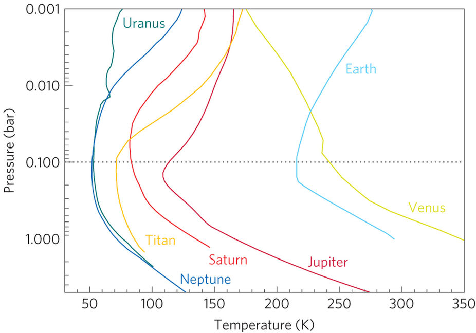
As discussed above, the deepest parts of atmospheres are dominated by the infrared opacities, that makes the radiation transport poorly effective. In the case of giant planets, main source of infrared opacity is represented by the collision-induced absorption (CIA) of molecular hydrogen. For other cases, infrared opacity is largely dominated by a minor constituent of the atmosphere (methane for Titan, carbon dioxide for the Earth), that turns out therefore to have a major impact on the overall thermal structure of the planet. At the approximate pressure level of 1 bar, mean IR opacity of the Solar-System atmospheres is still in the range between 2 and 9. Only at lower pressures, when opacity becomes in the order of unity, radiation can be effectively emitted toward deep space. This is the approximate level where the boundary between convective and radiative region is located.

At higher altitudes, opacity at shorter wavelengths (UV) become dominant over IR opacity. The latter is indeed critically dependent upon pressure, given the dependence of CIA and line broadening upon pressure. Opacity at shorter wavelengths is due to a number of minor components (notably methane and ozone) that experience photo dissociation, with a net deposition of energy from the Sun directly into the atmosphere, with an increase in air temperature that creates the observed stratosphere (as defined by the positive lapse rate). Robinson & Catling (2014) demonstrated that in the case of upper atmospheres with a short-wave optical depth much greater than infrared optical depth, the stratopause develops - for a large range of conditions - at the approximate level of 0.1 bar. The same study indicates that stratopause develops always well inside the radiative region of the atmosphere.

2 Physical and chemical changes in planetary atmospheres

2.1 Origin of planetary atmospheres

Table LABEL:tab:4_tab_02 summarizes the mean composition of planetary atmospheres of the Solar System, at the respective surfaces or at the approximate 1 bar level for the giant planets.

Table 2: Mean troposphere composition (volume percentages) and surface pressure of atmospheres of the Solar System. Updated from NASA Planetary Fact Sheets (https://nssdc.gsfc.nasa.gov/planetary/factsheet/)

Atmospheres of rocky planets are believed to be largely “secondary”, i.e.: formed by out gassing of planetary interior after that the original gaseous envelope, accreted during the planet formation, was removed by the action of solar radiation and wind in the early life of the Sun or by impacts. While the weak gravity fields of rocky planets could possibly justify the gravitational escape of lighter elements such as Hydrogen and Helium, this would leave behind substantial (albeit not intact) amount of heavier noble gases, in amounts well above the trace levels currently observed. Later contributions to the secondary atmospheres from impacts (notably, comets) may also have been important. Given the large variety of present-day conditions observed in rocky planets, subsequent evolution – directly or indirectly driven by the distance from the Sun – has also been fundamental.

Figure 2: Elemental enrichment with respect to the Solar composition in the atmospheres of giant planets. Courtesy PSL/ Univ. of Michigan (http://clasp-research.engin.umich.edu/psl/research.html). For an updated version, see Figure 2.1 in atreya:2018.

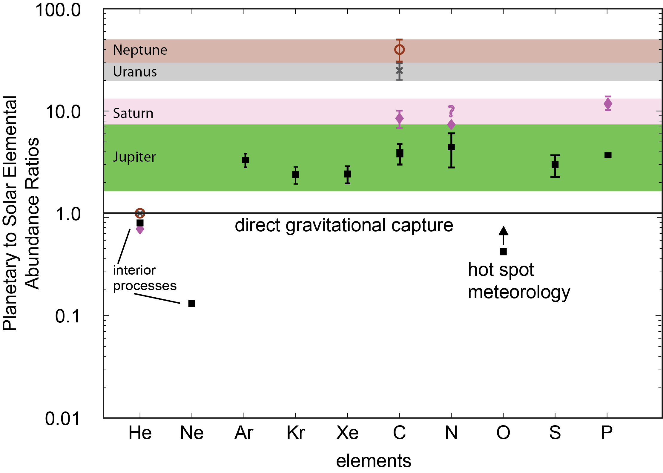
For giant planets, the comparison of elemental abundances observed in atmosphere against the ones inferred for the Sun may provide key constraints on the formation scenarios (Figure 2). Best experimental evidence is currently available for Jupiter, where a direct sample was performed by the Galileo Entry Probe during its descent on Dec 7^th, 1995. Overall, heavy elements appear to be enriched consistently by a factor 3 with respect to the mean solar composition, that would been contrarily expected in the case of a direct capture of material from the proto-solar nebula by direct gravitational accretion. The observed enrichment suggests therefore that a central core of the proto-Jupiter must have formed firstly. Only in subsequent phases, its gravitational attraction shall have been sufficient to attract planetoids rich in volatile elements (in forms of “ices”) but lacking the hydrogen envelop due to their very low masses. Composition data are much more fragmentary for Saturn, where an enrichment of a factor 10 can be inferred from a limited number of infrared active molecules and for Uranus and Neptune, where an enrichment of about 30 is assumed on the solely basis of the estimate of carbon (in the form of methane). An extensive discussion on these aspects is provided by (atreya:2018). Ices are expected to have contributed in much larger extent to the formation of Uranus and Neptune (“icy giants”) with respect to Jupiter and Saturn cases (“gas giants”). Indeed, albeit most external layers of icy giants are still formed mostly of Hydrogen and Helium, heavier elements are thought to represent a substantial fraction of planetary interiors, as demonstrated by their mean densities, with values of 1.27 and 1.63 g cm³ , similar to the Jupiter value (1.32 g  cm³), despite the much lower degree of internal compression.

For the cases of rocky planets, extensive volcanism is expected to have occurred at the beginning of the Solar-System existence, as a result of the dissipation of the internal heat, which was accumulated by impacts during the accretion phase and by decay of radioactive materials. Inference of the composition of the secondary atmospheres from the measurements on current volcanic gas releases on Earth volcanoes is however prone to substantial uncertainties. Most of volcanic activity on present-day Earth is associated to subsidence of oceanic crust and presents therefore substantial enhancement in water and carbon content associated to reprocessing of ocean floors. Possibly more representative are outgassing from “hot-spot” volcanoes away from plate boundaries, assuming that they originated at the core-mantle interface. In these cases, an enrichment in sulphur (a supposed component of the core) shall be expected. Despite large variability among different samples, hot-spot outgassing consist primarily of carbon dioxide (up to 50%), water (up to 40%) and sulphur dioxide (Symonds et al., 1994). Role and timing of post-formation impacts to the overall inventory of volatiles in the atmospheres of rocky planets is still matter of debate. The value observed for the hydrogen isotopic ratio D/H in the water of Earth oceans is about one third of that determined to exist in comet 67P (altwegg:2015), albeit substantial uncertainties exist on the overall significance of available cometary estimates with respect to the overall population of these objects. Conversely, the D/H ratio in carbon-rich chondroid meteorites matches quite well the Earth’s values, pointing to a possible role of these reservoirs in forming the atmospheres of rocky planets (morbidelli:2000).

2.2 Loss mechanisms for planetary atmospheres

A substantial fraction of the atmospheric mass of a planet can be removed during its evolution by several different mechanisms:

• Jeans thermal escape: in regions where Knudsen number approaches one, there is a tail in the Maxwellian distribution of air particles speeds that exceeds escape velocity. Corresponding air particles can be lost in space since further collisions are rare and they behave as ideal projectiles. The fraction of air particles with speed modules between $v$ and $v+dv$ is given by

  $$f(v)dv=const\,N\left(\frac{m}{k_{\rm B}T}\right)^{\frac{3}{2}}\,v^{2}\,e^{-\frac{m\,v^{2}}{2\,k_{\rm B}\,T}}dv\,,$$ (27)

  where $m$ is the mass of the molecule ($m=\mu_{\rm a}u$). The efficiency of loss depends therefore both on atmosphere temperature as well as on air particle mass. This may eventually result in variations of isotopic ratios of a given species with respect to their original values (isotopic fractionation), the effect being more evident in lighter species.

Hydrodynamic escape: it occurs when heavier atoms, which are not expected to be efficiently removed on the basis of the Jeans escape, are subject to a high number of collisions from escaping lighter atoms. Heavier species are therefore effectively dragged away from planet atmosphere by momentum transfer. The mechanism requires a very high rate of Jeans escape over lighter species, a condition not currently seen in Solar System atmospheres. It is expected to become important in the very hot atmospheres of exoplanets and having been significant in the earliest phases of rocky planets evolution. • Impact erosion: the impact of large bodies (with sizes of the order of atmospheric scale height) may eject ballistically a seizable fraction of the atmosphere. Air molecules/atoms with speeds exceeding the escape velocity are lost in space. This mechanism is not expected to produce substantial isotopic fractionation. • Sputtering: individual air particles may achieve speeds exceeding the escape velocity upon collision with energetic neutral particles (ENA) or ions originating outside the atmosphere. • Solar wind sweeping: atmospheric particles previously ionized by UV radiation or by the impinging of energetic particles are trapped in the magnetic-field lines of the Solar wind moving in the vicinity of upper ionosphere. The mechanism is important for planets not protected by a significant intrinsic magnetic field, such as Venus and Mars. The mechanisms listed above remove permanently the atmospheric mass from the planet. However, the atmosphere can also be substantially depleted by a variety of other mechanisms that fix – permanently on temporary – a specific component of the atmosphere to the surface of the planet. Most important are condensation (notable examples are the water on the Earth to form oceans or the seasonal cycle of condensation/sublimation of carbon dioxide at the Mars poles) and chemical fixation (such as formation of carbonate or iron oxide deposits).

2.3 Evolution of the atmospheres of rocky planets

Evolution of the Earth atmosphere

A key factor on the evolution of Earth climate has been represented by the occurrence of large bodies of liquid water at the surface. This is due to the suitable orbital position of the planet, since closer distance to the Sun would have implied higher atmospheric temperatures and would have let the water in the form of steam. The presence of water was functional in removing substantial amounts of carbon from the atmosphere of the early Earth. The solution of carbon dioxide in water and subsequent reaction with silicate rocks are key steps leading eventually to the trapping of carbon in seabeds in the form of carbonates. An example can be the following

$${\rm CO}_{2}(aq)+{\rm H}_{2}{\rm O}\rightarrow{\rm H}_{2}{\rm CO}_{3}(aq)$$

$${\rm Ca}{\rm Si}{\rm O}_{3}(s)+2{\rm H}_{2}{\rm CO}_{3}(aq)\rightarrow{\rm Ca}^{2+}(aq)+2{\rm HCO}^{-}_{3}(aq)+{\rm H}_{2}{\rm SiO}_{3}(aq)$$

$$2{\rm HCO}^{-}_{3}(aq)\rightarrow{\rm CO}_{3}^{2-}(aq)+{\rm H}_{2}{\rm O}+{\rm CO}_{2}(aq)$$ (28)

$${\rm Ca}^{2+}(aq)+{\rm CO}_{3}^{2-}(aq)\rightarrow{\rm Ca}{\rm CO}_{3}(s)$$

Current estimates on carbon pools expect the total amount trapped as carbonates to exceed by a factor about $5\times 10^{4}$ the present day atmospheric content (falkowski:2000). If released in the atmosphere as carbon dioxide, this would create a CO₂ dominated atmosphere with a surface pressure exceeding the one observed in Venus.

Another key step in the evolution of Earth atmosphere was the release of large amounts of molecular oxygen in the atmosphere. This was strictly linked to development of early life forms that evolved biological cycles producing free-oxygen as discard product. An example is the current form of photosynthesis, presented here in a strongly simplified form, that is

$$6{\rm CO}_{2}+6{\rm H}_{2}{\rm O}\rightarrow{\rm C}_{6}{\rm H}_{12}{\rm O}_{6}+6{\rm O}_{2}\,.$$ (29)

The molecular oxygen was initially fixed in rocks, oxidizing exposed iron-bearing minerals and forming the so called “red-bed formations” found worldwide. Once the geological sinks became saturated, the molecular oxygen begun to accumulate in the atmosphere. Availability of molecular oxygen lead to the creation of the ozone layer and to the oxidation of residual amounts of methane still present in the Earth atmosphere.

Evolution of the Venus atmosphere

Albeit it is reasonable to assume that evolution of Venus started from conditions rather similar to those on the Earth, a substantial difference has been represented by the proximity to the Sun. It is generally assumed that liquid water may have existed on the surface during the earliest phases of Venus history (until 2 Gy ago). Nevertheless, the capture of carbonates has not been so effective as on the Earth since solubility of CO₂ decreases with increasing liquid temperature. The persistence of carbon dioxide in the atmosphere would have progressively risen the temperature and make the ocean evaporation more effective. The process has a positive feedback, being water vapour a greenhouse gas as well. This eventually resulted in a progressively faster rise of temperatures until the oceans completely evaporated (“runaway greenhouse”). If kept in the atmosphere, water vapour is more easily dissociated by UV radiation in the uppermost tropospheric levels. Given the low mass of hydrogen atoms, they are easily lost to space due to Jeans escape (ingersoll:1969). Moreover, given the lack of substantial magnetosphere at Venus, ionized hydrogen atoms are more easily swept away by the Solar wind. A substantial loss of water in the Venus atmosphere is demonstrated by the D/H ratio measured in the very small amounts of water still present in the atmosphere, being this value about 150 times higher than the one observed on the Earth. This observation is consistent with the preferential loss of light species associated to the Jeans escape. Moreover, direct measurements of ion loss from Venus demonstrated that still today H⁺ and O⁺ are lost in space in stoichiometric ratios corresponding to those of water (fedorov:2011).

Evolution of the Mars atmosphere

Surface of Mars bears clear evidence of the occurrence of liquid water in the geological past, but actual size of possible large water bodies on the surface is still matter of debate. Albeit gamma ray spectrometry has revealed that substantial amounts of war ice must exist in form of permafrost ice beneath the Mars surface (boynton:2002), the current surface pressure of the planet does not allow to sustain the occurrence of liquid water; consequently, long term climate changes shall have occurred along Mars history. Estimates based on argon isotopes confirm that the planet atmosphere shall have experienced a minimum loss of about $70\%$ in mass (jakosky:2017). The low mass of the planet shall have played a role in such a massive loss, enhancing Jeans escape. Impact erosion by large bodies was another factor. Recent measurements by the MAVEN satellite suggest however that erosion by solar wind represented the single most important factor in the evolution of Mars, another object that lacks intrinsic magnetic field. MAVEN data detected spikes in the atmospheric escape during energetic plasma coronal mass ejections from the Sun. These events are believed to have occurred much more frequently in the early life of the Sun and may have therefore represented a major cause of atmospheric loss for Mars (curry:2017).

2.4 Photochemistry

The photo dissociation of atmospheric molecules by UV solar radiation represents a key factor in shaping the chemical cycles occurring in planetary atmospheres. In oxidative environments, such as the ones of rocky planets, the most important species is atomic oxygen, due to its high electro negativity. In reducing environments, such as the one found in giant planets, the dissociation of carbon and nitrogen bearing species (methane and ammonia respectively) and lack of strong oxidants allow the development of complex chemical patter and the production of a variety of heavier molecules. An extensive discussion on the subject is provided by Yung & de More (1999).

Venus and Mars

The photodissociation involves the main atmospheric component

$${\rm CO}_{2}+h\nu\rightarrow{\rm CO}+{\rm O}\hskip 28.45274pt\lambda<2050\,{\rm\AA}\,.$$ (30)

In the thin Martian atmosphere, the reactions occur efficiently down to the surface. On the thicker atmosphere of Venus, the maximum production rate is expected at about 60 km above the surface. The direct inverse reaction is extremely slow, since it requires a third molecule M to be involved, that is

$${\rm CO}+{\rm O}+{\rm M}\rightarrow{\rm CO}_{2}$$ (31)

Despite the very different rates of these reactions, the carbon dioxide mixing ratios remains much above the expected levels in the atmospheres of both planets, pointing toward the existence of other mechanisms to replenish the CO₂ content. In both cases, catalytic cycles involving minor components have been identified.

In the Martian environment, odd oxygen produced from the trace amounts of water vapour (again by photodissociation reactions) is involved in the reaction

$${\rm CO}+{\rm OH}\rightarrow{\rm CO}_{2}+{\rm H}\,.$$ (32)

Notably, the overall cycle balance is such that no net loss of water vapour occurs at the end of the cycle, where water acts therefore as a catalyst.

In the Venus environment, the recombination involves chlorine, a trace component confined in the lower troposphere because of the efficient condensation of chloride acid (the main Cl-bearing species) in the lower clouds:

$${\rm Cl}+{\rm CO}+{\rm M}\rightarrow{\rm ClCO}+{\rm M}$$

$${\rm ClCO}+{\rm O}_{2}+{\rm M}\rightarrow{\rm ClC(O)O}_{2}+{\rm M}$$ (33)

$${\rm ClC(O)O}_{2}+{\rm Cl}\rightarrow{\rm CO}_{2}+{\rm ClO}+{\rm Cl}$$

Venus Express measurements confirmed global scale patterns in the distribution of CO consistent with a creation at high latitude, equatorial locations and subsequent transport and destruction at lower altitudes, poleward positions.

Giant Planets

Methane is dissociated by photons with $\lambda<1625$ Å. In the typical Jupiter conditions the photodissociation occurs at pressure levels with $p<10^{-3}$ bar. Despite the low densities found there, the tendency of carbon to catenation results in a wide range of organic molecules being produced, most abundant being C₂H₆ (ethane) and C₂H₂ (acetylene). In Jupiter, despite air temperatures warm enough to forbid the methane condensation, a substantial depletion of methane occurs between the $10^{-7}$ and $10^{-8}$ bar levels, where concentration of photodissociation products is expected to peak. In the atmosphere of the icy giants, condensation of methane is expected to occur at levels much deeper that those affected by photodissociation. Therefore, the detection of organic molecules in the stratosphere of both Uranus and Neptune has been interpreted as a possible evidence of the occurrence of vertical motion transporting methane to its own dissociation levels.

Ammonia is also effectively photo dissociated by photons with $\lambda<2300$ Å. In this case, an important product is represented by hydrazine

$${\rm NH}_{3}+h\nu\rightarrow{\rm NH}_{2}+{\rm H}$$ (34)

$${\rm NH}_{2}+{\rm NH}_{2}\rightarrow{\rm NH}_{4}$$

Since hydrazine is expected to experience prompt condensation in the conditions met in the upper atmospheres of giant planets, it is invoked as a key component of high altitude hazes observed in these environments (see also Sect. LABEL:4_sec:4.3).

In the Jupiter atmosphere, the above reaction (Eq. 34) is expected to occur at much deeper levels ($200-300$ mbar) than the one affecting methane. This is due to the deeper penetration of the less energetic photons affecting ammonia as well as the substantial condensation experienced by ammonia in the upper troposphere. Nonetheless, occasional rises of ammonia caused by large storms at levels enriched (by downward diffusion) in acetylene are invoked as a scenario to create compounds containing nitrile ($-$CN), isonitrile ($-$NC), or diazide ($-$CNN) groups, possibly responsible of the colours observed for features such as the Great Red Spot (carlson:2016).

2.5 Aerosols

Without any exception, all atmospheres of the solar system in collisional regime ($R_{\rm n}<<1$) contain – at least occasionally – aerosols. In the great majority of cases, these aerosols are formed by the condensation of atmospheric gaseous species, being often minor components.

The condensation of gases can occur when the partial pressure $P_{\rm p}$ of a gas exceeds the equilibrium pressure between the gaseous and the liquid/solid phase. The equilibrium pressure is usually approximated by the Clausius–Clapeyron relation

$$\ln{P_{\rm eq}}=-\frac{L}{R_{\rm gas}T}+C\,,$$ (35)

being $R_{\rm gas}$ the gas constant, $T$ the air temperature, $L$ the specific latent heat of vaporization/sublimation and $C$ a constant. Both $L$ and $C$ are characteristic parameters of a gas. This formula immediately demonstrates how the condensation critically depends upon air temperature and partial pressure of the involved species, both factors being - at least at local scale - sensitive to an high number of different dynamical factors. The approximation in Eq. (35) is valid for temperatures well below the critical temperature of the considered species.

Albeit Eq. (35) describes the possibility for condensation to occur, more extensive treatment is needed to characterize the growth of the dimensions of aerosol particles. For liquid aerosols, homogeneous nucleation occurs when vapor directly condense to form droplets. On the basis of considerations upon Gibbs free energy (Salby, 1996), it is possible to demonstrate that molecules tend to re-evaporate until the droplet reaches a critical radius $r_{\rm c}$

$$r_{\rm c}\propto\frac{2\,\sigma}{k_{\rm B}\,T\,\ln{\frac{P_{\rm p}}{P_{\rm eq}}}}\,,$$ (36)

being $\sigma$ the surface tension. Only when the critical radius has been exceeded, the droplets tend to increase by diffusion of vapour through the droplet boundary.

In heterogeneous nucleation, the vapour molecules condensates initially over other type of aerosols, reaching therefore much more easily the critical radius required to overcome the surface tension. The heterogeneous nucleation represents therefore the key mechanism to initiate aerosol condensation in actual atmospheres. Ionization induced by magnetospheric precipitation or cosmic rays can induce droplet charging and enhance substantially the condensation processes in the upper atmospheres. In matter of fact, above the critical radius, growth of droplets is substantially modified by the reciprocal collisions, that becomes the dominant factor in later stages of droplet growth.

Beside condensation products, other types of aerosols are typically found in planetary atmospheres. They include: volcanic ashes, the products of surface erosions (dust clouds on Mars and Earth), the hydrodynamic emissions along gases from surface (geysers on Enceladus and Triton) and meteoric dust.

The role of aerosols in the atmosphere physics can hardly be overestimated:

• their capability to reflect incoming solar radiation and to adsorb IR radiation may alter substantially the overall energetic balance of an atmosphere;

the absorption/release of latent heat may alter the energetic balance at local level; • the condensation and gravitational precipitation of aerosol modify substantially the vertical distribution of minor species; • aerosol can act as effective catalytic sites for a number of atmospheric chemical reactions. Moreover, emerging radiation field is modified substantially by aerosol scattering, with major implications on remote sensing methods.

3 Fundamentals of atmospheric dynamics

3.1 Main drivers

Planetary atmospheres experience large scale motion of air masses. In the small bodies (rocky planets, Titan, Pluto, Triton), the main driver for motions is represented by the differential heating of surface and atmosphere induced by different latitudinal exposure to Solar irradiation. In the giant planets, the effects due to the dissipation of internal heat become more and more important toward the interior.

The wind patterns caused by pressure differences are however substantially modified by the planet rotation and more specifically by the need for air parcels to preserve their angular momentum. Other factors to take into account in assessing the global circulation of a body are:

• differential heating of surface induced by the contrast between land and oceans (on the Earth) or between high and low albedo areas (e.g. Mars);

mass flow on condensible species (CO₂ on Mars, N₂ and CH₄ on Pluto and Triton); • seasonal cycles, with particular attention to axial tilt and orbital eccentricity. The discussion in this section largely follows the introduction provided by depater:2010. Further details are can be found in Salby (1996, chapter 12).

3.2 Global circulation patterns

Figure 3: General scheme of the General circulation on Earth troposphere. Courtesy NASA/Wikimedia Commons.

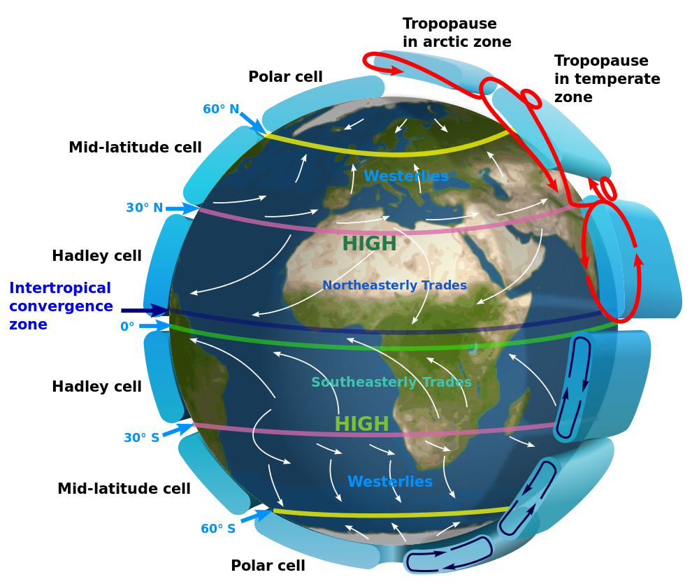
A common feature of atmospheric circulation in planetary atmospheres is the so-called Hadley circulation (Figure 3). In the case of rocky planets, the heating of the surface at the subsolar latitudes leads to an expansion of air parcels, that become buoyant and rises in altitude, cooling during expansion and reaching levels where IR cooling become effective. During the rise, air tends to lose the condensible component to form aerosols: the release of latent heat further enhances the circulation. Once in altitude, the air parcels are subject to a net pressure gradient that leads them poleward. During this latitudinal motion, air parcels must preserve their angular momentum despite a lesser distance from planet rotation axis and therefore accelerates along parallels in the same direction of planet rotation. On the Earth this eventually leads to the formation of subtropical jets. At higher latitudes, air parcels (strongly depleted in condensible species) eventually sinks again toward the surface, heating by adiabatic compression. At low altitudes the air parcels are subject to a reverse pressure gradient (created by the ascending branch of the cell) and flows toward the sub solar regions. This surface flow must still preserve angular momentum and is therefore accelerated along parallels in the direction opposed to planet rotation.

The longitudinal extension of the cell is dependent upon temperature gradients at the surface as well as on the rotation speed. The very slow rotation of Venus and negligible axial tilt allow the Hadley circulation to develop in two symmetric, hemisphere-wide cells. A similar condition is found on Mars around equinoxes. On the Earth, the proper Hadley cell is extended approximatively up to latitudes of $30^{\circ}$. Another conceptually similar cell (polar cell) exist beyond $60^{\circ}$, similarly driven by surface temperature gradients. At intermediate temperate latitudes, the weak Ferret cell with an opposite circulation pattern can be found. This structure is essentially driven by the dragging of Hadley and polar cells at its boundaries, being its behavior (it transfers heat toward equator) thermodynamically adversed. Gaseous giants display similarly a large number of cells in both hemispheres, marked by strong jets at their boundaries. Structure of icy-giant circulation is known in a lesser degree, but is apparently characterized by a two larges cell in each hemisphere. It shall be stressed that meridional (i.e.: along meridians) and vertical motions associated to Hadley circulation are by far weaker than those associated to zonal (i.e.: along parallels) winds. On the Earth at the approximative level of 0.5 bar, vertical motions are usually well below the 1 cm s^-1 value, to be compared to mean zonal winds up to 25 m s^-1 at mid-latitudes.

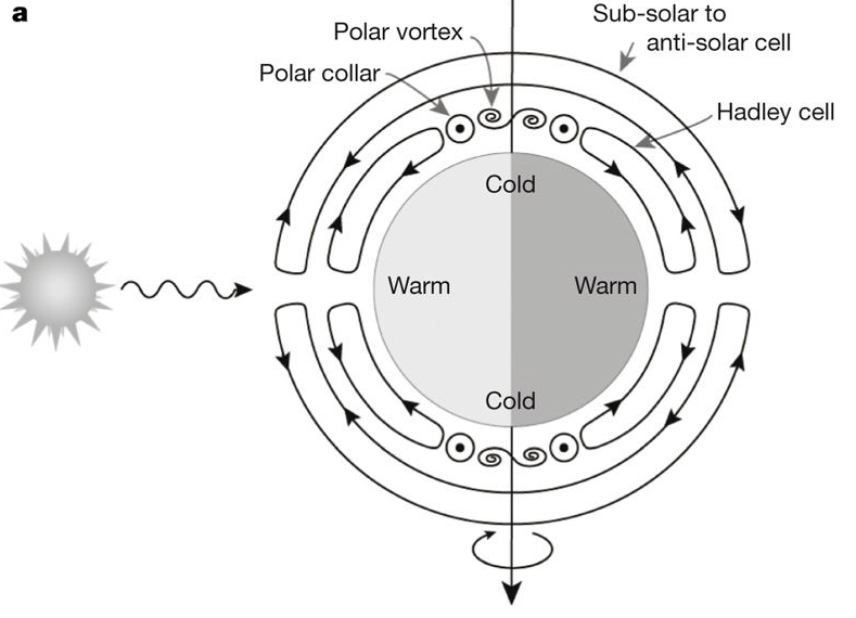
Another type of global circulation, driven solely by solar irradiation, is the transfer of air from the warm sub-solar point to the anti-solar point on the night side, with a mechanism conceptually similar to the Hadley cell. This kind of circulation occurs in the upper atmosphere, where drag and irradiation from surface become negligible and UV solar radiation can induce a substantial deposition of heat. In the Venus case (Figure 4), infrared observations has allowed to map directly the downwelling of UV dissociation products.

Figure 4: General scheme of the Solar/Antisolar circulation observed in the Venus’ upper atmosphere. Hadley circulation occurs simultaneously at altitude below $\approx 100$ km. Reprinted by permission from Macmillan Publishers Ltd: Nature, Svedhem et al. (2007), copyright 2007.

Another important feature related to global circulation is the dissipation of energy. In addition to the IR cooling mentioned earlier, an important role is played by the friction occurring in vicinity of surface in the planetary boundary layer. Here, turbulence may play an important role in transferring the energy from large scale eddies with scales comparable to the roughness of surface down to Kolmogorv scale length where molecular diffusion can dissipate it efficiently.

3.3 Wind equations

To describe numerically the winds, we start from the Navier-Stokes equation, Eq. (9), considering the rotating reference frame represented by planet surface. We denote the speed in this reference frame $\overrightarrow{u^{\prime}}$. In this case

$$\rho\frac{D\overrightarrow{u^{\prime}}}{Dt}=-2\,\rho\,\overrightarrow{\omega\vphantom{\nabla}}_{\rm rot}\times\overrightarrow{u^{\prime}\vphantom{\nabla}}+\rho\,\overrightarrow{g^{\prime}\vphantom{\nabla}}-\overrightarrow{\nabla}p-\overrightarrow{\nabla}\cdot\left(\mu\overrightarrow{\nabla}u^{\prime}\right)$$ (37)

being $\overrightarrow{\omega}_{\rm rot}$ the rotation angular speed of the planet. Naming as $u$, $v$ and $w$ the wind components along the meridians, parallels and the vertical direction, respectively, and neglecting viscosity we get:

$$\frac{Du}{Dt}=2\,\omega_{\rm rot}(v\,\sin{\theta}-w\,\cos{\theta})-\frac{1}{\rho}\frac{\partial P}{\partial x}$$

$$\frac{Dv}{Dt}=2\,\omega_{\rm rot}\,u\,\sin{\theta}-\frac{1}{\rho}\frac{\partial P}{\partial y}$$ (38)

$$\frac{Dw}{Dt}=2\,\omega_{\rm rot}\,u\,\cos{\theta}-g-\frac{1}{\rho}\frac{\partial P}{\partial z}\approx 2\,\omega_{\rm rot}\,u\,\cos{\theta}$$

where $\theta$ is the latitude and where, in the last formula, we have introduced the assumption of hydrostatic equilibrium, Eq. (12). In the so-called shallow atmosphere approximation, motions along the vertical directions are considered negligible on the basis of dimensional analysis (Salby 1996, Sect. 11.4.2) and, considering only the horizontal plane, we get

$$\frac{Dv}{Dt}=f_{\rm C}\overrightarrow{v}\times\hat{z}-\frac{1}{\rho}\overrightarrow{\nabla}P\,,$$ (39)

where $\overrightarrow{v}$ is the speed vector on the horizontal plane, as seen in the rotating reference frame, $f_{\rm C}\equiv 2\,\omega_{\rm rot}\,\sin{\theta}$ is the Coriolis parameter and $\hat{z}$ the unit vector normal to the surface. Heuristically, the Coriolis term expresses the conservation of angular momentum of air parcels as they move between different latitudes.

A further important approximation can be made considering a balanced flow, where the Coriolis and pressure gradient terms compensate each other leading to a steady flow $(Dv/Dt=0)$ in the geostrophic approximation. In these circumstances,

$$v=\frac{1}{\rho f_{\rm C}}\left(\hat{n}\times\overrightarrow{\nabla}P\right)\,,$$ (40)

being $\hat{n}$ the unit vector normal to speed, implying that flow occurs along isobars. The jets forming at the descending branches of Hadley cells are the important examples of geostrophic balance.

If we introduce the geopotential $\Phi_{\rm g}$

$$\Phi_{\rm g}=\int_{0}^{Z}gdz=-\int_{P_{0}}^{P}\frac{dP}{\rho}\,,$$ (41)

we can reformulate the previous discussion referring to isobaric surfaces and to restate Eq. (40) as

$$v=\frac{1}{f_{\rm C}}\hat{n}\times\overrightarrow{\nabla}_{{\rm P}}\Phi_{\rm g}\,,$$ (42)

where index $P$ indicates the gradient as computed over isobaric surfaces. Upon differentiation of Eq. (40) with respect to pressure and inserting Eq. (13) leads to

$$\frac{-\partial v}{\partial\ln{P}}=\frac{R_{\rm gas}}{f_{\rm C}}\hat{n}\times\overrightarrow{\nabla}_{{\rm P}}T\,.$$ (43)

Namely, this thermal wind balance relates the latitudinal variation of temperatures with the vertical variations of zonal winds. Heuristically, in presence of a longitudinal temperature gradient, vertical spacing between isobaric surfaces tends to increase toward warmer areas, in a greater amount at greater altitudes. The net effect is an increased slope of isobaric surfaces with increasing altitude. At a fixed altitude, this implies an increased pressure gradient and the need of stronger winds to compensate the pressure difference. Thermal wind balance represents a common method to estimate winds (gradients) from maps of air temperature as a function of latitude and altitude away from equatorial regions when no direct wind measurements are available. Thermal wind is also the main driver of mid-latitude jets observed on the Earth (as explained above, sub-tropical jets are mostly driven by conservation of angular momentum at the descending branch of the Hadley cell).

Eq. (39) can be separated in the normal and tangential components of the motion to achieve the following:

$$\frac{dv}{dt}=-\frac{1}{\rho}\frac{d\rho}{ds}$$ (44)

$$\frac{v^{2}}{r}=-f_{\rm C}v-\frac{1}{\rho}\frac{dP}{dn}\,,$$

being $s$ the curvilinear coordinate along the motion and $v$ the speed magnitude. This formulation allows one to consider balanced flow also in the cases where $f_{\rm C}$ is very small, such as in the vicinity of equator or in slow rotating planets. Namely, this cyclostrophic balance occurs when the pressure gradient along the direction normal to the flow is balanced by the centrifugal term. Important examples are the atmospheric super rotations observed in the atmosphere of Venus and Titan.

We can define the relative vorticity of a velocity field as

$$\omega_{v}=\overrightarrow{\nabla}\times\overrightarrow{u\vphantom{\nabla}}\,,$$ (45)

The vorticity field expresses a measure of the tendency of the fluid to rotate around the point of interest. For an air parcel at rest with respect to the planet surface, it holds $|\omega_{v}|=2\omega_{\rm rot}$. Vorticity is particularly important in the description of eddies. Namely, common features of planetary atmospheres are represented by large vortices, where air tends to rotate around a local maxim/minimum of pressure. Cyclones are the vortices developing around a pressure minimum, while anticyclones are the vortices develop around a pressure maximum. The region where air is actively forced to rotate behaves approximatively like a rigid body, with tangential speeds proportional to distance from the center. Here vorticity has a non-zero value. On the outer parts, essentially dragged by the vortex core, the tangential speed tends to decrease as $1/r$, being $r$ the distance from center. Here vorticity becomes zero. In cyclonic circulation, the Rossby number allows one to estimate if either geostrophic or cyclostrophic balance holds. It is defined as

$$R_{0}=\frac{v}{L\,f_{\rm C}}\,,$$ (46)

where $v$ is the magnitude of the wind speed and $L$ a characteristic scale of the phenomenon (such as vortex diameter). With $R_{0}<<1$, the geostrophic approximations can be considered valid and pressure gradient is essentially balanced by the Coriolis acceleration. Small-scale systems (small $L$) or those developing at low latitudes are more easily dominated by centrifugal effects. With considerable simplifications, we can define the Rossby potential vorticity as

$$\omega_{pv}=\frac{\omega_{v}+f_{\rm C}}{l}\,,$$ (47)

being $l$ a quantity proportional to the thickness of the layer involved in the motion. Potential vorticity gives a measure of the angular momentum of fluid around the vertical axis. Once the turbulent dissipation occurring at planetary boundary layer is neglected, it can be demonstrated that potential vorticity of an air parcel must be preserved. A consequence of this requirement is that variations of latitudes (and hence of the Coriolis parameter) implies a variation of vorticity. The conservation of potential vorticity is also responsible for other phenomena such as the expansion of cyclones upon passing over topographic heights or their prevailing trajectories over Atlantic Ocean.

3.4 Atmospheric waves

The overall global circulation patterns described in previous sections are rarely found in these basic forms in actual planetary environments. Conversely, these shall be considered as idealized dynamical schemes that emerges once highly-variable temporary features are removed by averaging over time. Atmospheres actually hosts a variety of wave features (periodic variations of the physical parameters of the atmosphere in time and space), that can often be treated mathematically as infinitesimal perturbations of the steady flow regimes. Here we briefly describe only a few types.

Thermal tides

The thermal waves are created by the natural modulation imposed on solar input by the rotation of the planet (or by the possible super rotation of the atmosphere). Sun-radiation flux represents the effective forcing acting on the atmosphere. At a fixed location, its value versus time becomes abruptly null after the sunset (with a discontinuity in its first derivative). As typical of step-like functions, corresponding Fourier transform contains significant contributions from several harmonics of the fundamental period (in this case, the actual day length). More frequent periods are those associated to one day and half days. Most common tides appear as variations of air temperatures and altitudes of isobaric surfaces, being the variation phases approximatively fixed with respect to the sub-solar position and therefore seen as migrating by an observer on the surface. These includes, for example, the periodic variations of surface pressure clearly seen on Mars and air temperature minima/maxima locked at fixed local time positions on Venus.

Rossby waves

Development of weather systems on the Earth mid-latitudes is often dominated by the so-called Rossby waves. Considering the Earth north hemisphere case, an air parcel, involved in the strong polar estward jet, can experience small longitudinal variations. Preservation of potential vorticity will modify its relative vorticity, representing an actual restoration factor: an initial displacement northward (decrease of Coriolis factor) will reduce relative vorticity, until it becomes negative and the air parcels effectively move back southward. Upon overshooting, the same potential vorticity conservation principle initially increases the potential vorticity, until it surpasses the initial value of Coriolis parameters and is deviated toward north. An observer moving westward would see the air to spin clockwise while moving north and clockwise while moving south. This mechanism creates the meander-like wind flow patterns often observed at mid-latitudes.

Gravity waves

Gravity waves are vertical perturbations of the atmosphere where gravitation and buoyancy plays the role of restoration forces. Considering the case of an infinitesimal vertical displacement of the atmosphere, this can result in periodic oscillations at Brunt-Väisälä frequency

$$\nu_{\rm BV}=\sqrt{-\frac{g}{\rho_{0}}\frac{\partial\rho(z)}{\partial z}}\,,$$ (48)

being $\rho_{0}$ the air density at the initial level in the unperturbed atmosphere.

Eq. (48) leads to a real value of the Brunt-Väisälä frequency – i.e. to periodic oscillations – only when density decreases with altitude. In the opposite case, perturbations of the system are amplified exponentially – i.e. the atmosphere is gravitationally unstable. Gravity waves are typically induced by a flow upon a topographic discontinuity, and as such has been observed on the Earth, Mars and – unexpectedly – Venus. They can however develop also in absence of topographic discontinuity (notably in giant planets) in a large range of instabilities in the stratification of the atmospheres.

3.5 Diffusion

In Sect. 3.2 we briefly described the motion of air parcels. The turbulence, usually found at the lowest atmospheric levels, ensures that atmosphere remains well mixed, i.e. with an uniform composition over altitude. At low Reynolds numbers $R_{\rm e}$, Eq. (11), however, molecular diffusion, driven by the random motion of individual molecules, can create substantial deviations from the well-mixed conditions.

Namely, the motion of the molecules of a given chemical species is such to remove any gradient in its density as well in the temperature field. Moreover, given the dependence of Eq. (14) on molecular mass, lighter species tends to exhibits higher values of scale height $H_{i}$ and to be more uniformly distributed in altitude with respect to heavier ones. At the same time, the eddy diffusion by turbulence tends to remove any compositional gradient. Quantitatively, the flux $\Phi_{i}$ of the molecules of the generic chemical species $i$ across a horizontal surface is given by

$$\Phi{i}=-N_{i}D_{i}\left(\frac{1}{N_{i}}\frac{\partial N_{i}}{\partial z}+\frac{1}{H_{i}}+\frac{\alpha_{i}}{T(z)}\frac{\partial T(z)}{\partial z}\right)-N\,K\frac{\partial(N_{i}/N)}{\partial z}\,,$$ (49)

being $N$ the total molecular number density, $N_{i}$ the molecular number density of the species $i$. $D_{i}$ is the molecular diffusion coefficient for $i$ (in turn, inversely proportional to $N$) while $K$ is the eddy diffusion coefficient (roughly proportional to $R_{\rm e}$). This latter term is such to remove any gradient in the mixing ratio of the species.

4 Atmospheres of individual Solar System bodies

Our review of atmospheres of the Solar System considers the bodies that own significant parts of their atmosphere in collisional regime

4.1 Rocky planets

Rocky planets are characterized by solid surfaces composed mostly of silicates. Interaction with the overlying atmospheres takes place mostly in the form of release of volcanic gases (Earth and likely Venus), molecular diffusion trough the soil and deposition/sublimation of polar caps (Earth and Mars). Moreover, surfaces represent the lower boundary of atmospheric circulation and the site of important chemical reactions involving atmospheric components. Table LABEL:tab:4_tab_03 summarizes the key properties of the atmosphere of rocky planets in the Solar system.

Table 3: Properties of the Solar-system rocky planets that are more relevant for the discussion on their atmospheres. Taken from the NASA Planetary Fact Sheets (https://nssdc.gsfc.nasa.gov/planetary/factsheet/).

Available at http://helper.ipam.ucla.edu/publications/kttut/kttut_8441.pdf

Piccialli A., Tellmann S., Titov D. V., Limaye S. S., Khatuntsev I. V., Pätzold M., Häusler B., 2012, Icarus, 217, 669

Piccioni G., Drossart P., Sanchez-Lavega A., et al., 2007, Nature, 450, 637

Plainaki C., Milillo A., Mura A., Orsini S., Massetti S., Cassidy, T., 2012, Icarus, 218, 956

Robinson T. D., & Catling D. 5C., 2014, Nature Geoscience, 7, 12

Salby M. L., 1996, Fundamentals of atmospheric physics (Academic Press)

Sayanagi K. M., Dyudina U. A., Ewald S. P., et al., 2013, Icarus, 223, 460

Sayanagi K. M., Dyudina U. A., Ewald S. P., et al., 2014, Icarus, 229, 170

Shematovich V. I., Johnson R. E., Cooper J. F., Wong M. C., 2005, Icarus, 173, 2

Showman A. P., & Dowling T. E., 2000, Science, 289, 1737

Smith M. D., 2004, Icarus, 167, 148

Smith, M. D., Lapedes A. S., de Jong J. C., et al., 2004, Science, 306, 371

Sromovsky L. A., de Pater I., Fry P. M., Hammel H. B., Marcus P., 2015, Icarus, 258, 192

Svedhem H., Titov D. V., Taylor F. W., Witasse O., 2007, Nature, 450, 629

Symonds R. B., Rose W. I., Bluth G. J. S., Gerlach M., 1994, Reviews in Mineralogy and Geochemistry, 30, 1

Titov D. V., Taylor F. W., Svedhem H., et al., 2008, Nature, 456, 620

Titov D. V., et al., 2016, in Venus III, ed. by B. Bezard, (Cambridge University Press)

Turrini D., Politi R., Peron R., et al., 2014, 104, 93

Webster C. R., Mahaffy P. R., Atreya S. K., et al., 2015, Science, 347, 415

Yung Y. L., & de More W. B., 1999, Photochemistry of Planetary Atmospheres (Oxford University Press)