Automated detection of very Low Surface Brightness galaxies in the Virgo Cluster

Abstract

We report the automatic detection of a new sample of very low surface brightness (LSB) galaxies, likely members of the Virgo cluster. We introduce our new software, DeepScan, that has been designed specifically to detect extended LSB features automatically using the DBSCAN algorithm. We demonstrate the technique by applying it over a 5 degree² portion of the Next-Generation Virgo Survey (NGVS) data to reveal 53 low surface brightness galaxies that are candidate cluster members based on their sizes and colours. 30 of these sources are new detections despite the region being searched specifically for LSB galaxies previously. Our final sample contains galaxies with $26.0\leq\langle\mu_{e}\rangle\leq 28.5$ and $19\leq m_{g}\leq 21$, making them some of the faintest known in Virgo. The majority of them have colours consistent with the red sequence, and have a mean stellar mass of $10^{6.3\pm 0.5}M_{\odot}$ assuming cluster membership. After using ProFit to fit Sérsic profiles to our detections, none of the new sources have effective radii larger than 1.5 Kpc and do not meet the criteria for ultra-diffuse galaxy (UDG) classification, so we classify them as ultra-faint dwarfs.

1 Introduction

The low surface brightness (LSB) universe is one that can be easily overlooked due to observational biases (Disney, 1976), yet remains an important test-bed for the enduring paradigm of the $\Lambda$CDM universe. It is theorised that a significant portion of the missing baryon budget (Shull et al., 2012) may be hidden in diffuse sources such as intra-cluster light (ICL) (Mihos et al., 2017), tidal streams (Cooper et al., 2010; Mowla et al., 2017) and LSB galaxies (LSBGs), an idea supported by the surprising abundance of ultra-diffuse galaxies (UDGs) originally detected in the Coma cluster (van Dokkum et al., 2015; Koda et al., 2015).

A great deal of effort has been devoted to searching for diffuse sources in other cluster environments, including the Virgo cluster (Davies et al., 2016; Mihos et al., 2005; Mihos et al., 2015); the Fornax cluster (Kambas et al., 2000; Muñoz et al., 2015) and others (e.g. Janssens et al., 2017; Román & Trujillo, 2017), as well as in the vicinities of massive galaxies (Javanmardi et al., 2016; Müller et al., 2017). LSB galaxies are also expected to form and exist in the field (McGaugh, 1996; Di Cintio et al., 2017; Amorisco & Loeb, 2016) along with an ultra-diffuse intra-group baryonic component (Driver et al., 2016).

Of particular contemporary interest is the origin of the UDG. It is a matter of ongoing debate whether they can be described as “failed L* galaxies” (van Dokkum et al., 2017), tidally puffed-up dwarfs (Collins et al., 2013) or the natural expectation of high spin dwarfs predicted from $\Lambda$CDM cosmology (Amorisco & Loeb, 2016). Whatever the case, the issue has prompted several authors to search for LSB galaxies in a multitude of environments (van der Burg et al., 2016; van der Burg et al., 2017; Román & Trujillo, 2017). One promising explanation has emerged indicating that UDGs may originate from dwarf galaxies that were quenched early on (Beasley & Trujillo, 2016), but statistical significance has been hampered by the inability to reliably detect very LSB objects other than by visual inspection (Muñoz et al., 2015; Venhola et al., 2017).

Modern deep imaging surveys such as the Next Generation Virgo Survey (NGVS) (Ferrarese et al., 2012), Next Generation Fornax Survey (NGFS) (Muñoz et al., 2015), KiDS (de Jong et al., 2015), and HSC-SPP (Aihara et al., 2017) provide deep multi-wavelength data sets capable of probing the LSB Universe. Such data sets may offer a treasure trove of LSB objects, but it seems that current methodology has limited the ability for them to be fully exploited. While by-eye extraction of LSB sources currently has the very desirable advantage of minimal contamination from artefacts in the data, the sheer size of modern data means that only very small regions can be analysed this way. Upcoming surveys such as Euclid and LSST make this approach completely infeasible for the future.

One of the main issues for LSB science is the quality of the data and its reduction. Slater et al. (2009) have made progress in removing artefacts caused by internal reflections of bright stars by modelling the point spread function (PSF) to high accuracy and out to wide radii. Further progress has been made in constructing very deep image stacks with special attention to preserving LSB features (Blanton et al., 2011; Fliri & Trujillo, 2015; Mihos et al., 2017). Despite these advances, many efforts to identify LSB features automatically have relied on methods that are sub-optimal for the extraction of low signal-to-noise ratio (SNR) sources. The most common of these is SExtractor (Bertin & Arnouts, 1996), which at its core identifies objects as contiguous regions above the sky distribution at some confidence level. Davies et al. (2016) have shown that it tends to systematically miss or fragment large, diffuse objects even with settings optimised to the detection of LSB objects.

Despite its popularity, there are alternatives to SExtractor. Some examples include Clumpfind (Williams et al., 1994), FellWalker (Berry, 2015) and others, but again these are not optimised to detect LSB objects and suffer from similar issues to SExtractor. This has motivated several authors to create their own algorithms such as Oddity (Butler-Yeoman et al., 2016, and references within), MTObjects (Teeninga et al., 2016) and NoiseChisel (Akhlaghi & Ichikawa, 2015). An increasingly popular approach (e.g. Zheng et al., 2015) is to detect objects via a watershed segmentation algorithm, whereby detections can grow larger and larger until they reach a saddle point in intensity. This approach is also used by the ProFound software (Robotham et al., 2018).

The above alternatives (with the exception of ProFound, which is new) have not yet been widely used in the literature. Given the current abundance of research into the LSB Universe, we have been prompted to develop another detection package, called DeepScan. This has been developed to meet the following criteria:

• The software should supersede SExtractor in its ability to detect extended LSB structure.

• Detection limits should be quantifiable so that the completeness of samples can be estimated.

• The algorithm should adapt to the various shapes of LSB sources e.g. LSBGs and ICL.

• The software should be intuitive and simple to use in a modern scripting language.

• The inputs and outputs of DeepScan should be compatible with those of other software.

• The algorithm should be as efficient as possible and be written to take advantage of parallel processing methods.

Our software implementation has been developed to run as efficiently as possible in order to cope with present and futuristic big-data challenges. The public availability of deep, wide-area survey data such as that of KiDS and VIKING (Edge et al., 2013) (each covering thousands of square degrees with sub-arcsecond pixels) means that DeepScan can be used immediately. Such survey data will make good testing grounds for the software, which we hope to apply to even larger surveys such as Euclid and LSST.

This paper is intended to inform the reader of the methodology behind DeepScan. We will endeavour to provide an up-to-date user’s manual where the code is hosted publicly at https://github.com/danjampro/DeepScan with a GPLv3 license. The paper is organised in the following way: In section 2, we give an overview of the algorithm at the core of the detection method. In section 3 we give a brief overview of the DeepScan software, with the full documentation made available online. We note that during the development of DeepScan, Greco et al. (2017) have also developed a pipeline aiming to detect low surface brightness features using SExtractor. While this work is quite similar in its objectives and methods, some of the differences between the two pieces of software are discussed in section 4. In section 5 we give an example of its application to the publicly available NGVS data to reveal a sample of exceptionally faint galaxies. The sample retrieved from this analysis can provide a training-set for comparisons with other methods like ProFound. Finally we discuss plans to increase the area of sky we have explored in this work.

While in this paper we primarily discuss the identification of LSB galaxies, the detection method employed by DeepScan makes no assumptions about the underlying morphologies of its detections. It can therefore be used to detect other extended LSB sources such as tidal streams or intra-cluster light.

2 DBSCAN in astronomy

DBSCAN (Density-based spatial clustering of applications with noise, Ester et al., 1996), is a two-parameter algorithm that is designed to identify regions of high density within an $n$-dimensional data set. The algorithm has found recent use in astronomy through the classification of eclipsing binaries (Kochoska et al., 2017) and the morphological analysis of open clusters (Bhattacharya et al., 2017). Broadly speaking, our application of DBSCAN operates in a similar way to SExtractor in that it builds detections by clustering together nearby pixels above some brightness threshold. In both cases, the detections are statistically unlikely to occur due to fluctuations in the background.

The fundamental difference between our use of DBSCAN and SExtractor is that a DBSCAN detection is based on the density of pixels above a SNR threshold within its $\epsilon$ radius, whereas SExtractor builds its detections by identifying contiguous regions of pixels with significant flux, possibly on a smoothed image. (We note that SExtractor can amalgamate non-contiguous sources in its “cleaning” stage, which attempts to remove noise peaks that have been detected in the halos of brighter objects).

The first parameter of DBSCAN is a clustering scale length ($\epsilon$) and the second ($\eta$) is the minimum number of data points required within an $\epsilon$ radius for a cluster to form. The algorithm iterates over every input data point. If the number of points $\varphi$ within a circular radius of length $\epsilon$ meets the condition $\varphi\geq\eta$, the point is marked as a core point; this is the basic building block of a cluster. Then, each point enclosed within $\epsilon$ (known as secondary points) is checked to see if they also meet the condition to be core points, and if so then they are added to the same cluster. Thus, a cluster can contain more than one core point. This process repeats until there are no more core points to add to the cluster and it is complete. The algorithm then repeats the process to identify separate clusters within the dataset, if they exist. The clustering process is illustrated in figure 1.

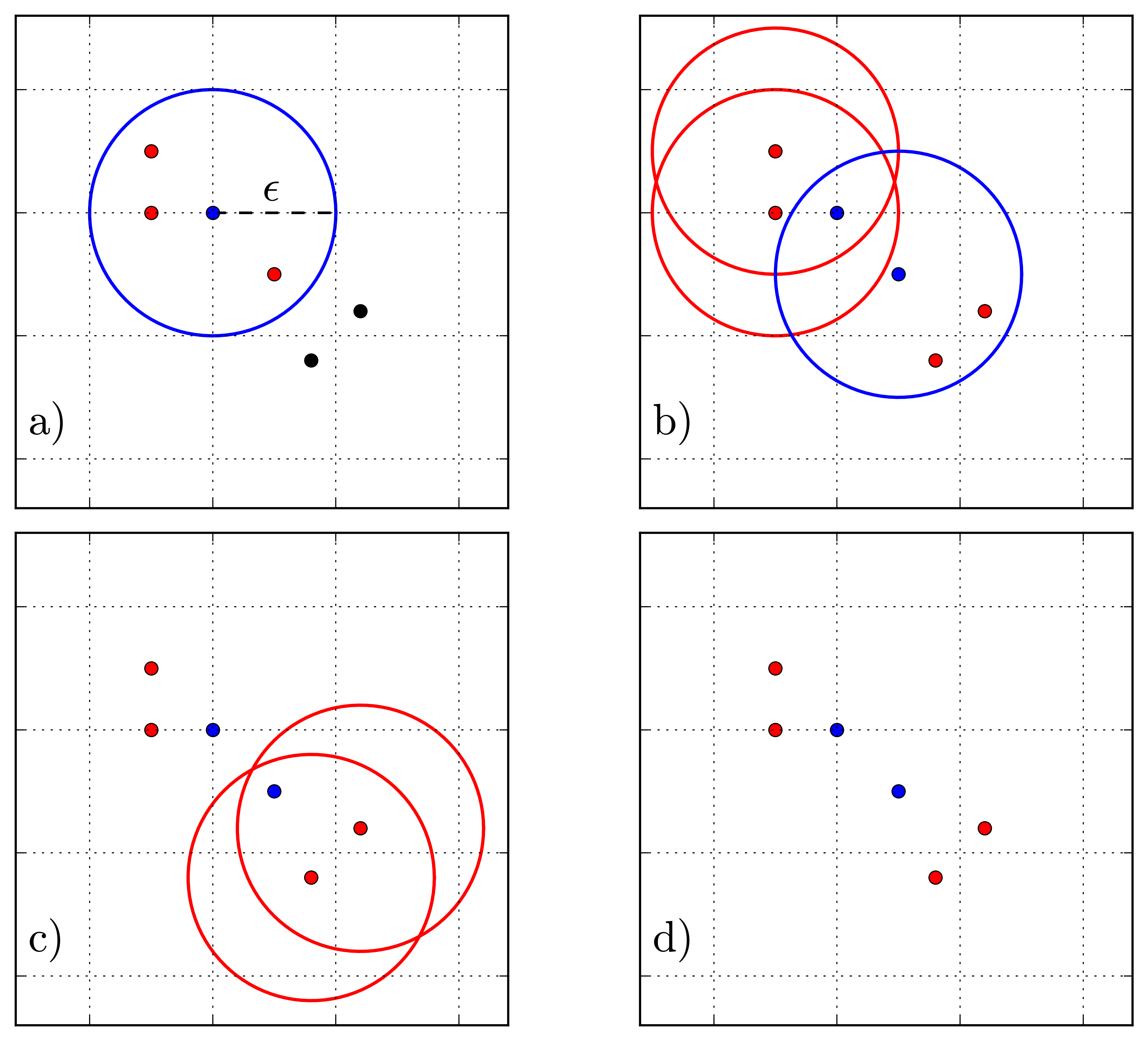
Figure 1: A visualisation of the DSBSCAN algorithm with $\eta$=3. In a), the algorithm proceeds to identify a core point (blue). Then in b) it checks each of the secondary points (red) to see if they meet the criteria to be a core point - this is true of one of the secondary points, which is also shown in blue. The secondary points of the new core point are checked in c), and the final cluster, consisting of two core points, is shown in d).

Our approach is to use the spatial coordinates of pixels above a brightness threshold as inputs to DBSCAN, essentially identifying sources as over-densities of these pixels. This is analogous to how resolved LSB galaxies are detected through over-densities of their stars against the background. While we have not implemented usage of the upper detection threshold $I_{max}$ in DeepScan, we include it in the modelling for completeness.

The circular nature of the search aperture used in DBSCAN means that the algorithm has a “resolution” determined by $\epsilon$. This limitation does not rule out the detection of elongated structures if they are significant over scales similar to or larger than $\epsilon$. The algorithm therefore performs poorly in identifying objects significantly smaller than the detection circle and in separating sources closer together than 2$\epsilon$. While the former point is addressed by allowing the sensitivity of the algorithm to be set by the user, the latter could be remedied with a de-blending or segmentation routine. We have not implemented such a routine as instead we rely on the low spatial density of LSB objects and a high quality source mask to mitigate source confusion (see $\S$3.3).

The sensitivity of DBSCAN is set by $\eta$. To derive a value for $\eta$, a value of $\epsilon$ is assumed that remains a hyper-parameter of the algorithm (i.e. a parameter that is set by the user). $\eta$ is estimated with the assumption that the noise brightness distribution is a zero-mean Gaussian of standard deviation $\sigma_{n}$, i.e.:

$$P(I_{n})=P(I_{n},\mu=0,\sigma=\sigma_{n})$$ (1)

for noise intensity $I_{n}$, mean $\mu$ and standard deviation $\sigma$. If a brightness threshold is applied with lower and upper boundaries $I_{min}$ and $I_{max}$ ($\mu_{min}$ and $\mu_{max}$ in magnitudes per square arcsecond) respectively, the pixel-to-pixel noise distribution can be used to predict the probability $P_{thresh}$ of a background pixel with a true brightness of $I_{b}$ lying within the threshold:

$$P_{thresh}=P(I_{min}\leq I\leq I_{max})=\int_{I_{min}-I_{b}}^{I_{max}-I_{b}}P(I_{n}^{\prime})dI^{\prime}$$ (2)

Thus, an accurate model of the background is also assumed. As the amount of noise per pixel is modelled as an independent random variable, the binomial distribution can be used to calculate the number of pixels expected to lie within the brightness threshold within a circular region of radius $\epsilon$. In the hunt for LSB objects, $\epsilon$ should be large so that it encapsulates a high number of pixels. Therefore the binomial distribution can be approximately represented by another Gaussian,

$$P(\varphi)=P(\varphi,\mu_{\varphi},\sigma_{\varphi})$$ (3)

with

$$\mu_{\varphi}=P_{thresh}N_{pix}$$ (4)

$$\sigma_{\varphi}=(P_{thresh}(1-P_{thresh})N_{pix})^{\frac{1}{2}}$$ (5)

where $N_{pix}$ is the number of pixels enclosed by a circle of radius $\epsilon$, and $\varphi$ is the number of those pixels within the threshold. Equation 3 can be integrated between $\varphi^{\prime}$ and $N_{pix}$ to find the probability $P_{0}$ of $\varphi^{\prime}$ or more pixels in the circle lying within the threshold:

$$P_{0}=\frac{1}{2}\left[\operatorname{erf}\left(\frac{N_{pix}-\mu_{\varphi}}{\sigma_{\varphi}\sqrt{2}}\right)-\operatorname{erf}\left(\frac{\varphi^{\prime}-\mu_{\varphi}}{\sigma_{\varphi}\sqrt{2}}\right)\right]$$ (6)

Setting $\varphi^{\prime}$=$\eta$ and rearranging for $\eta$, we obtain

$$\eta=\sigma_{\varphi}\sqrt{2}\operatorname{erf}^{-1}\left[\operatorname{erf}\left(\frac{N_{pix}-\mu_{\varphi}}{\sigma_{\varphi}\sqrt{2}}\right)-2P_{0}\right]+\mu_{\varphi}$$ (7)

We can replace the hyper-parameter $\eta$ with a new parameter $\kappa$ , defined as the number of standard deviations (equation 5) above the expected number of points enclosed within $\epsilon$. We can therefore write the somewhat simpler expression,

$$\eta=\mu_{\varphi}+\kappa\sigma_{\varphi}$$ (8)

where $\kappa$ is in one-to-one correspondence with the probability $P_{0}$.
Equation 7 describes the number of pixels lying within the brightness threshold, within a circle of radius $\epsilon$ embedded within pure Gaussian noise. It is useful as it expresses $\eta$ as a function of the probability of that many pixels occurring due to noise, a probability that can be set arbitrarily low by increasing $\kappa$. It also allows the prediction of what should be detected by the algorithm. For example, In the context of galaxy detection the detectable region on the central surface brightness (CSB), magnitude plane can be calculated. The brightness profiles of galaxies are often described by the Sérsic profile (Graham & Driver, 2005), which can be expressed as:

$$I(r)=I_{0}\exp{\left(\frac{-r}{h}\right)^{\frac{1}{n}}}+I_{b}$$ (9)

for radius $r$, CSB $I_{0}$ ($\mu_{0}$ in magnitudes per square arcsecond), scale size $h$ and Sérsic index $n$. $I_{b}$ is the background brightness. In analogy to equation 2, the probability of finding a pixel within the brightness threshold is:

$$P_{thresh}(I(r))=\int_{\Delta I_{min}}^{\Delta I_{max}}P(I_{n}^{\prime})dI^{\prime}$$ (10)

with

$$\Delta I_{\begin{subarray}{c}min\\ max\end{subarray}}=I_{\begin{subarray}{c}min\\ max\end{subarray}}-I(r)$$ (11)

Equation 10 can be integrated over a circular region to obtain

$$\varphi_{s}=\pi\int_{0}^{\epsilon}{r\left[\operatorname{erf}\left(\frac{\Delta I_{max}}{\sigma_{n}\sqrt{2}}\right)-\operatorname{erf}\left(\frac{\Delta I_{min}}{\sigma_{n}\sqrt{2}}\right)\right]dr}$$ (12)

The condition for the galaxy to be detected is then simply:

$$\varphi_{s}\geq\eta$$ (13)

Numerical approximations to this condition are shown for a variety of values of $\epsilon$ in figure 2. We show similar plots for $\kappa$ and the Sérsic index $n$ in the appendix.

The effects of the PSF have not been modelled here. While the PSF is in general non-analytical and varies between datasets (and even in the same dataset), we probe the effects of a typical seeing PSF for ground based wide-area surveys in $\S$2.1 and have found the effect to be negligible for our target sources.

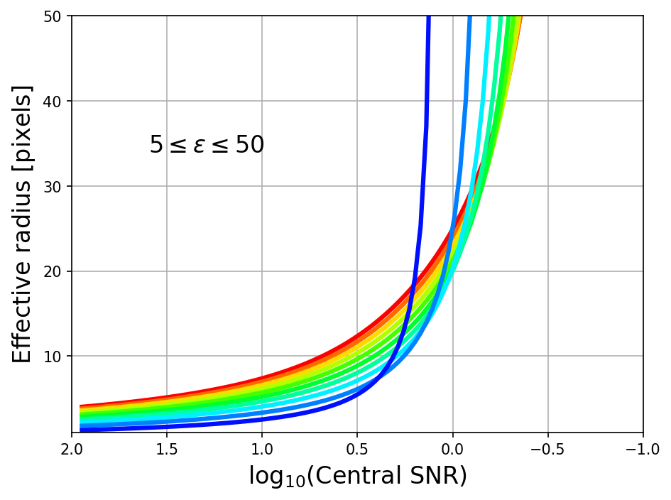
Figure 2: Variation of the limits of detection with $\epsilon$, ranging between 5 (blue) and 50 pixels (red), with a colour gradient showing intermediate linearly-spaced values of $\epsilon$ increasing with redness. These results were obtained with $\kappa$=10, $I_{min}$=$\sigma_{n}$. The PSF and the effects of photon noise are not considered in this plot.

.

2.1 Testing DBSCAN

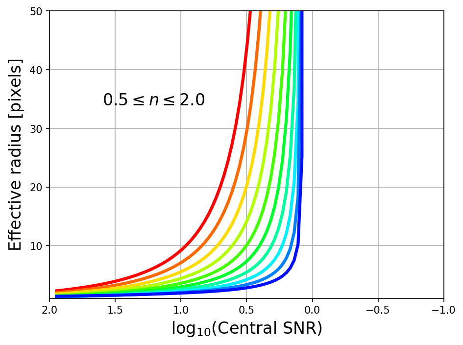
Figure 13: Variation of the limits of detection with $n$, ranging between 0.5 (blue) and 2 (red), with a colour gradient showing intermediate linearly-spaced values of $n$ increasing with redness. These results were obtained with $\kappa$=10, $I_{m}in$=$\sigma_{n}$, $\epsilon$=5 pixels

In order to demonstrate the validity of the statistical modelling presented in section $\S$2 we have performed artificial galaxy experiments, wherein sets of randomly generated circular Sérsic profiles ($n$=1) were generated using ProFit (Robotham et al., 2017) and hidden in random noise of RMS=$\sigma_{n}$. $n$=1 was used because it is a fiducial value for dwarf galaxies (e.g. Koda et al., 2015) (but also see figure 13). We also include the effects of photon noise in the experiments and assume a gain of 1. A large grid of profiles was produced and embedded into random noise, using central surface brightnesses defined by their signal-to-noise (SNR) ratio (SNR logarithmically drawn between 0.1 and 100). The profiles have effective (half-light) radii between 1 and 15 pixels, where we have converted between Sérsic quantities using the prescriptions of Graham & Driver (2005).

Individual profiles were spaced by eight times the maximum effective radius of the sample, and were each truncated at 4 times this radius. This was to ensure that extended profiles could not contribute to their neighbour’s detections.

Our new DBSCAN implementation (see $\S$3.1) was then applied to the synthetic image, and any synthetic source that had an object located (by the mean coordinate of the core points) within twice its effective radius was regarded as detected. No two DBSCAN detections could be assigned to the same source and it was asserted that there were no DBSCAN detections that did not have matches. This check was to ensure that large portions of the image had not been detected as one. Results from matching the detections with their profiles are shown in figure 3 for $\kappa$=10, $\epsilon$=5 pixels and a lower detection threshold of 1$\sigma_{n}$. Also on the plot is shown a numerical approximation (using the Nelder-Mead minimisation algorithm to the condition in equation 13). Importantly, the detection boundary predicted through the modelling is in good agreement with the observation of the synthetic data.

We have performed the same experiment after convolving the Sérsic profiles with a mock Gaussian PSF with a full-width at half-maximum (FWHM) of 5 pixels (typical for 1$\arcsec$ seeing with a 0.2$\arcsec$ pixel size). The results were practically identical, even for the lower values of effective radii that we probed. This is easily explained from the fact that $\epsilon$ was also 5 pixels. Of course, as the PSF FWHM becomes larger than $\epsilon$, we would expect to see a retraction of the detection boundary. However, DeepScan is intended for use on wide-area survey data (which typically has seeing and pixel scales of the order of what is probed here) and relatively large values of $\epsilon$, so this effect is not considered important.

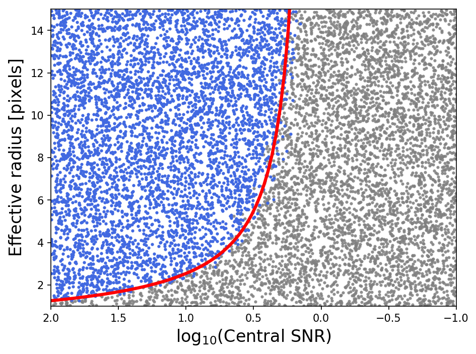
Figure 3: Results of the synthetic profile experiment for $n$=1 circular Sérsic profiles. Each point represents a synthetic source; blue ones have been detected and grey ones missed according to the criteria discussed in the text. The red line shows the boundary of detection predicted in equation 13. The sources presented here were not convolved with a PSF (see text).

The preceding derivation of $\eta$ also does not consider the effects of correlated noise. This is noise that is “clumpy”, produced during image stacking (interpolation, drizzling etc.) and from sources such as faint background galaxies that have not been accounted for in the sky modelling. In particular, this correlation will tend to make the uncertainty in the number of points contained within $\epsilon$ due to the sky distribution (equation 5) an underestimate. The degree of noise correlation varies between datasets, making its effects difficult to quantify in general. For our current purpose of getting an estimate for $\eta$, the effects of underestimating $\sigma_{\varphi}$ can be accounted for by using higher values of $\kappa$, as can be seen in equation 8. To estimate the degree to which $\kappa$ should change to accommodate the correlation, we generated independent random noise and applied a Gaussian filter with $\sigma$=1 pixel to create noise correlated over scales of two pixels. In such a set-up, Monte-Carlo trials suggest the standard deviation in equation 5 is underestimated by a factor of $\sim$2.5 and thus $\kappa$ would have to be multiplied by this factor to obtain equivalent behaviour to the uncorrelated case in terms of robustness against the detection of noise peaks (this comes at the cost of sensitivity).

Despite this, the assignment of $\kappa$ is likely to be done empirically rather than derived statistically because even with a source mask in place there will likely be unmasked sources contributing to a non-Gaussian background (see $\S$5.3).

There are similarities between DBSCAN and conventional data smoothing techniques because of the size of the search radius $\epsilon$. One major reason why very large smoothing kernels are not commonly used for detection is because nearby objects become confused with each other. Further, smoothing over bright, concentrated sources may produce detections that appear similar to LSB galaxies. By applying the source mask ($\S$3.3) before the detection algorithm, this problem is alleviated and we can make use of the SNR obtained over larger areas without significant source confusion. DBSCAN is also more robust to the detection of small unmasked background objects because the input pixels are not flux-weighted; sources are forced to be significant over areas similar to the search area in order to be detected.

3 The DeepScan software

DeepScan is a Python package intended to identify regions of significant LSB light. The software uses a novel implementation of the DBSCAN algorithm that was created in order to operate much more efficiently than the standard. This efficiency is in-part due to many calls to integrated C code within numpy and scipy. One of the goals of DeepScan has been to be compatible with other pieces of software, and as such there is a lot of flexibility as to what can be input to the software in terms of, for example, user-generated background maps or object masks. Equally, the outputs of DeepScan such as segmentation maps and initial guesses on Sérsic parameters can be easily transferred and used by different tools. If however the user does not have ready-made background maps etc., the basic usage of DeepScan is as follows:

1. Measurement of the sky distribution to produce sky and sky RMS maps (implicit source masking).

2. Generation of a bright source mask (currently SExtractor is used to create masks).

3. Source detection on masked frames using DBSCAN.

4. Automatic measurement of detections.

There are two notable issues with this pipeline: 1) There is no source de-blending other than that of the source mask. The justification for this is that following appropriate source masking the spatial frequency of diffuse sources on the masked image is assumed to be low enough so that no de-blending is necessary; 2) Users are likely to want higher quality source measurements than the approximate ones provided with DeepScan. We envisage these measurements to serve as inputs into robust profile fitting algorithms like ProFit.

3.1 Novel DBSCAN implementation

An important feature of any detection algorithm is the runtime. Lower runtime helps users to fine-tune their parameters as well as enabling large data sets to be analysed over accessible (CPU) time-frames. Code optimisation usually proceeds by reducing the most significant time-consuming operation in the program; in the case of DBSCAN this is the region query, whereby the number of points within $\epsilon$ are counted for every data point. A simple implementation of DBSCAN may perform the region query by directly measuring the Euclidean distances from every input point to every other point and storing these distances in a symmetric distance matrix. This is inefficient in terms of memory as well as CPU time because every unique element of the matrix requires checking for every query. Indexing structures such as the R-tree (Guttman, 1984) are optimised for spatial queries and allow for a significant speed-up. Many DBSCAN implementations use this method, including those in scikit-learn and R.

However, our implementation is done in a much different manner that obtains equivalent results in notably shorter time-frames through a convolution approach. The basic procedure is the following:

1. Create a binary image where pixels above the detection threshold are assigned the value of 1 and all others 0. We term the detection threshold as thresh, which is quoted in units of the background RMS unless otherwise stated.

2. Convolve the result with a top-hat filter of unit height and radius equal to $\epsilon$. This step essentially counts the number of thresholded pixels within an $\epsilon$ radius of every pixel.

3. Threshold the resulting image at $\eta$ (derived from $\kappa$ and thresh), creating a binary image with non-zero pixels being DBSCAN core points.

4. Convolve the result with the same top-hat filter as in step 2. This connects regions corresponding to unique DBSCAN clusters. Set all non-zero pixels to 1.

5. Run a contiguous pixel clustering algorithm over the result. This assigns unique integer labels >0 to each DBSCAN cluster. The result of this is known as segmap_dilated, and bounds the regions contained by all the DBSCAN core and secondary points.

6. Perform a binary erosion on each object in segmap_dilated to obtain the contiguous areas bounded by the core points. The result is simply called the segmap. A segmentation map of only the core points (corepoints) can also be retrieved.

We note that an “erosion” refers to contracting a source’s segment with a kernel (in our case the top-hat filter of radius $\epsilon$); For each pixel making up a source’s segment, all pixels that are contained within the kernel’s footprint centred on that pixel are removed from the segment. A dilation is the opposite transformation. Hence the name “segmap_dilated” is appropriate because it can be obtained by performing a dilation on the segmap. The only time an erosion is performed by DeepScan is to create the segmap from the segmap_dilated.

The speed-up from the above approach compared to standard implementations stems from the fact that a) fast-Fourier transform (FFT) techniques can be used for the convolution steps and b) The need for the DBSCAN region query is removed and is replaced by a much more efficient contiguous-pixel clustering algorithm.

We have tested DeepScan v1.0 against the scikit-learn and R DBSCAN implementations (versions 0.18.2 and 1.1-1 respectively) on one processor, and find that this implementation is faster than both. The tests were performed on a mid-2013 MacBook Pro (2.5 GHz Intel Core i5) with 8GB of RAM, running OSX 10.12.6. We also note that we find the R implementation to be significantly faster than that in scikit-learn, but scikit-learn gives the option to run DBSCAN in parallel whereas R does not. For example, averaging over five runs for a 500$\times$500 NGVS $g$-band cut-out, the times are DeepScan: 0.3s, R: 0.3s and scikit-learn: 0.8s. Enlarging the image to 1000$\times$1000 pixels gives DeepScan: 3.5s, R: 6.0s and scikit-learn: 17.6s. Scaling up once again to 4000$\times$4000 pixels, this time letting DeepScan and scikit-learn use four processors, the results are DeepScan: 12.8s R: 27.6s and scikit-learn: 89.5s. We tested whether there was a difference between the output of DeepScan compared to the other implementations and found that there was an exact match between the results.

3.2 Sky measurement

DeepScan can produce sky and sky RMS maps if required. To obtain an estimate of the sky we iteratively make measurements of the sky and the sky RMS, each iteration using DBSCAN with a low detection threshold (default thresh=0.5) to identify sources (including LSB components) which are masked from the sky calculation in the following iteration. Using suitable values for $\epsilon$ (default of 5 pixels - similar to a typical PSF FWHM for wide field optical surveys) and $\kappa$ (default a value of 5 - low enough to encapsulate LSB components), this iterative masking reduces the bias incurred from unmasked LSB components each time. The iterations terminate when the sky level has converged to a user-specified tolerance. We have provided figure 4 as an example of the sky-measurement algorithm, which was generated with default parameters.

The sky and sky RMS levels are estimated in meshes. The mesh size is a user-defined parameter. We maintain flexibility by allowing custom estimators for the measurements, but by default use the median for the sky and a lower-quantile estimate of the RMS (i.e. the level for which 15.9% of the data is enclosed below the median). These are computed for each iteration, ignoring any masked pixels. The meshes are then median filtered over a customisable scale, before being interpolated over using a bi-cubic spline to the full image resolution. Meshes with too-few pixels are ignored in the interpolated over; by default at least 30% of the mesh must be unmasked to count. Following this, DBSCAN is run, and any pixel identified within the segmap_dilated is masked. The algorithm then checks for convergence on a mesh-by-mesh basis; individual meshes that have converged are ignored for further iterations and their converged values are used in the interpolation. This process repeats with the updated source mask, either until all the meshes have converged or a maximum number iterations has been reached (the default is 6).

We again emphasise that it is trivial to use sky and RMS maps generated externally from DeepScan. We also note that custom masks can be used as an input to the source masking routine, which can be combined with the mask generated with DBSCAN or even treated as the final mask, in which the iterative mask generation is not applied.

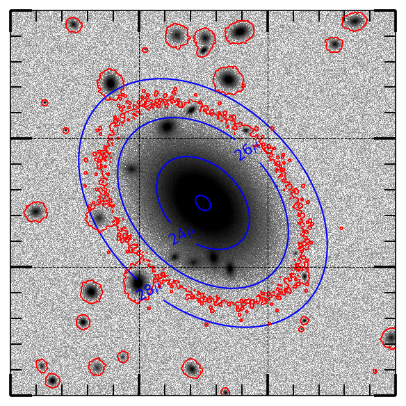
Figure 4: This shows a synthetic 1500$\times$1500 pixel image, with an extended central source and some smaller “background” objects. Contours of the surface brightness profile are shown (blue) for the central profile, as well as a contour showing the masked region (red). Clearly the mask extends to very low surface brightness (the RMS of the image is 26.2$\mu$). The 500$\times$500 pixel meshes (black dashed lines) were median filtered over 3$\times$3 regions. The actual sky level of the image was set to zero ADU. Despite the presence of the dominant LSB object in the frame, the maximum value of the sky was measured to be 28.4$\mu$ - well below the RMS level. The RMS was recovered with an accuracy of over 99%.

3.3 Masking bright sources

A crucial requirement of our detection method is a source mask. The mask must be created with the aim of eliminating all sources one does not wish to detect right out to their LSB halos. Our approach here has been to use SExtractor to create the source mask. Measurements from the output catalogue such as the FLUX_RADIUS were found to do a poor job, underestimating the source sizes even with high values of PHOT_FLUXFRAC (the fraction of light contained within the flux radius). This prompted us to model each source with a Sérsic profile and to size the ellipse according to some isophotal radius below the DeepScan detection threshold.

We estimated the Sérsic index without performing any additional fitting from the ratio between the effective and Kron radii (Graham & Driver, 2005). This is useful as both of these measurements can be efficiently retrieved by SExtractor with the KRON_RADIUS and the FLUX_RADIUS keywords and PHOT_FLUXFRAC=0.5. Combining these measurements with the total magnitude (also measured using SExtractor’s MAG_AUTO, by default with PHOT_AUTOPARAMS set to 2.5,3.5), the profile is fully characterised. The source is then masked in an elliptical aperture (based on SExtractor’s elliptical parameters) to the derived isophotal radius. We note that SExtractor allows the possibility to perform Sérsic fitting by requiring the SPHEROID_SERSICN or SPHEROID_REFF_IMAGE columns in the output file. While we have not explored this in our current work, it is possible that this would improve the fits at the expense of some computation time.

A caveat of the above approach is that galaxies typically have non-elliptical LSB components and therefore may not be adequately masked. It is likely that ProFound will eventually replace SExtractor for the source masking as it offers the advantage of non-parametric object masks as well as more reliable estimates of parameters such as the half-light radius (Robotham et al., 2018).

3.4 Source measurement

The goal of DeepScan is not to provide accurate profile fitting, but is rather to identify regions with significant LSB light. That said, we do provide a basic function for 1-dimensional Sérsic profile fitting in order to get initial estimates of parameters to input into robust 2D fitting programs such as ProFit. The basic requirements for the fit are the data and a segment corresponding to the source.

The initial task that is performed is the estimation of the centroid position and elliptical parameters (axis ratio and position angle). This is done using the same method of flux-weighted moments as in SExtractor (see Bertin & Arnouts (1996) for detail), where the user has the choice to calculate the moments on either a masked or unmasked segmentation map. The user can choose which of the three segmentation maps provided (segmap, segmap_dilated or corepoints) to calculate these parameters.

The next step is to measure the average (default median) flux within concentric elliptical annuli of fixed width centred on the source, based on the measurements from the previous step. The annuli iteratively increase their radius until a user-defined isophotal surface brightness is reached (often a relatively robust method of measuring large LSB galaxies) or a maximum radius has been reached. If the isophotal level is reached before sufficient steps have been performed then more steps will be taken in order to achieve a minimum number of data points (default is 5).

We then proceed to fit the profile using Scipy’s curve_fit routine, which by default uses the Trust Region Reflective algorithm for parameter optimisation in the case of constrained problems (each Sérsic parameter is constrained by default to have positive values). An initial parameter guess can be provided, but in its absence the parameters are estimated as following: The index $n$ is assumed as 1; The effective radius is assumed as the semi-major axis of the ellipse that bounds the segmentation map; the surface brightness at the effective radius is estimated by measuring the average surface brightness within the segmentation map, rescaling to effective surface brightness using the default value of $n$.

We have not yet implemented methods to measure non-galaxy like objects. However, we suggest the segmentation images outputted by DeepScan can be used as inputs to non-parametric measurement tools such as that offered in ProFound to provide estimates on parameters like total magnitude etc.

4 DeepScan vs Source Extractor

During our testing of SExtractor we have found that it can perform fairly well in detecting LSB features provided specific input parameters are used. In this section we describe some observations about its usage and explain why DeepScan may be preferred to detect specifically highly extended LSB objects. Our tests have consisted of us using a cut-out from the publicly available NGVS $g$-band data, which has a pixel size of 0.186$\arcsec$ and typical RMS of $\sim$26.9$g\mu$ with various combinations of SExtractor settings. For the experiment, both SExtractor and DeepScan used the same background mesh of 50$\arcsec$ ($\sim$270 pixels) that was median filtered in 3$\times$3 meshes (Using the BACK_SIZE and BACK_FILTERSIZE SExtractor keywords). The cut-out used had a size of 810$\times$810 pixels so that the background estimation was realistic. For this experiment, we have used SExtractor to convolve the image with a Gaussian kernel of 5-pixels RMS, as in Greco et al. (2017).

It is thought that the de-blending can routinely fragment large LSB features (Davies et al., 2016; Greco et al., 2017) (aka “shredding”). Indeed we have observed the de-blending fragmentation (figure 5a), which was observed with SExtractor’s de-blending contrast parameter DEBLEND_MINCONT=0.005 (the default). A way around the problem is to deactivate the de-blending by setting DEBLEND_MINCONT to 1 - this value is used for the remainder of our tests. We have not experimented with different values of DEBLEND_MINCONT in this work. We also note that it is important for the CLEAN parameter to be switched on (default) in order to reduce LSB source fragmentation, so it is activated in all our tests here.

Figure 5b) shows the result of increasing the value of DETECT_MINAREA (the minimum number of pixels required for a detection to count) compared to a). A much better job is done of identifying the LSB source as a single object, but we note that the detection suffers two problems: the shape of the segment corresponding to the LSB source is significantly perturbed by background objects; and spurious detections still exist around groups of background objects despite very high values of DETECT_MINAREA. Activating the de-blending here exacerbates the situation and the LSB source is missed entirely, with its flux being solely attributed to some of the background objects rather than any central object.

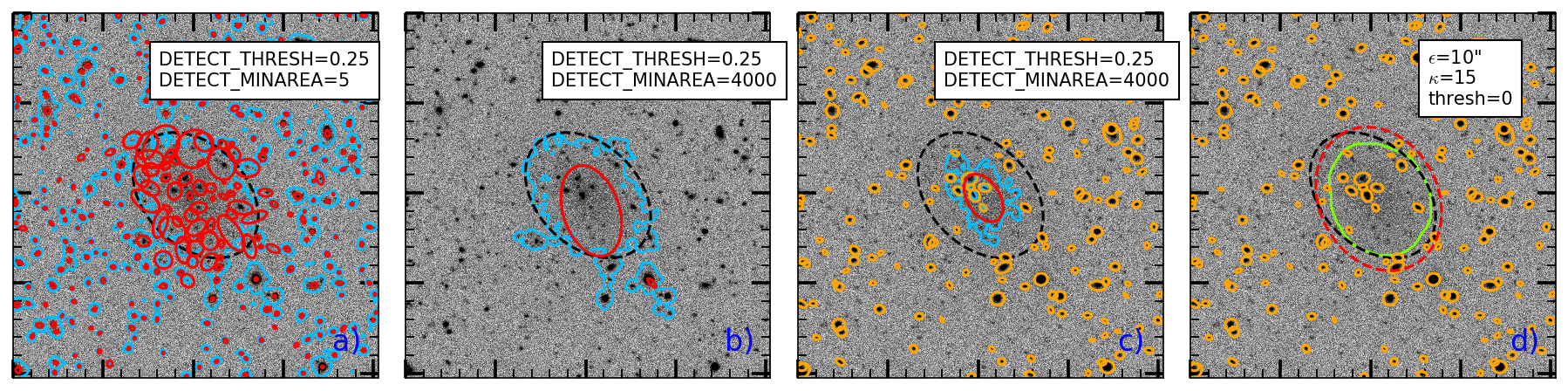
Figure 5: This is a real 810$\times$810 pixel NGVS data cut-out with a synthetic LSB galaxy with a convolved central surface brightness of $\sim$26.9$g\mu$ and an exponential profile ($n$=1) of effective radius 30$\arcsec$ (roughly equivalent to the lower size limit of a UDG at Virgo). The black dotted ellipse represents this source out to one effective radius. In frames a) to c), the light blue contour traces objects on the SExtractor SEGMENTATION check plot. The red ellipses represent SExtractor estimates of the effective radius for each detection, measured in the same way as in $\S$3.3. In figures c) and d), the orange ellipses bound the sources that are masked. In figure d), the green contour traces the DeepScan segmap, whereas the dashed red ellipse represents the effective radius as measured by DeepScan. See text.

Herein lies a downside of using SExtractor to detect LSB sources. The areas of the segmentation image corresponding to LSB objects detected on smoothed frames is made significantly unstable because of the presence of background objects that have either not been properly de-blended or have been erroneously assigned to the source in the cleaning stage. This is made clear by the morphology of the detection in figures 5b) and c). As this significantly effects the number of pixels an object contains, the usage of DETECT_MINAREA becomes an inherently unreliable tool to identify genuine LSB objects, yet is required to discriminate against background objects.

The problem is partially alleviated by applying a source mask to the image before its input to SExtractor as is also done by Greco et al. (2017) (note that there is no source mask handling within SExtractor) in that now the only detection that appears in the output catalogue seems to be associated with the LSB object itself rather than brighter objects in its vicinity. However, the problems associated with the LSB segment still exist - the segment is irregular and contains several unmasked background objects that significantly perturb it’s shape. It is also notable that the elliptical fit (determined by SExtractor’s half-light FLUX_RADIUS and elliptical parameters) does not do a reasonable job at measuring the object. This size underestimation can lead to the source being missed, as it is typical for authors to perform a cut on the minimum size of objects.

In contrast, the DeepScan detection (figure 5d) is much smoother and does a better job of tracing the shape of the LSB structure. It is arguable that this is because we used a large value of $\epsilon$ (10$\arcsec$=50 pixels), but we note that DeepScan is designed to work with such large kernels. The work of Greco et al. (2017) have also shown that using much larger kernels than 1$\arcsec$ is not feasible in SExtractor because of blending with unmasked faint/background galaxies (Koda et al., 2015; Sifón et al., 2018), although this could be improved with a better masking strategy. We also note in passing that SExtractor does not allow kernels larger than 31$\times$31 pixels, so it is impossible to use such a kernel from SExtractor. A second point of consideration is that the core points of the DeepScan detection define its shape, and these are identified as pixels with relatively high SNR on the original (i.e. non-smoothed) frame. Further, unmasked sources that cause the perturbations in the SExtractor segmentation map have less of an effect on the shape of the DeepScan detection because the pixels aren’t flux weighted in the DBSCAN algorithm.

To summarise, while it might be preferable to use DeepScan to trace extended LSB light it is also possible to use SExtractor to detect very low surface brightness objects, provided certain criteria are met:

1. A ready-made source mask is provided.

2. Large smoothing kernels are used (we note that the largest kernel size acceptable is 31$\times$31 pixels).

3. Large values of DETECT_MINAREA are used.

4. De-blending is deactivated.

5. One treats parameters derived from the SEGMENTAION check plot with some scepticism, particularly the FLUX_RADIUS as this seems to be systematically underestimated for large, diffuse objects.

6. Cleaning is on (CLEAN=Y) to avoid spurious detections.

5 Application to the NGVS

To demonstrate the DBSCAN algorithm we applied it to a subset of the publicly available NGVS data that we acquired from the Canadian Astronomy Data Centre. This data was taken with the square-degree MegaCam instrument on the Canada France Hawaii Telescope, and covers $\sim$100 square degrees of the Virgo Cluster in the $u,g,r,i,z$ bands. The NGVS was chosen because it offers deep imaging of the Virgo cluster at high resolution (0.186$\arcsec$ pixels), and was the same data used by Davies et al. (2016) with which we wish to compare. We use the $g$-band data as it has the best coverage, a low maximum seeing FWHM (1$\arcsec$) and an extended-source limit of 29$\mu$ (Ferrarese et al., 2012). The subset covers a five-degree² area projected radially eastwards from the centre of the Virgo cluster (i.e. M87). The subset is made from five overlapping frames, each covering an area of  1 degree² with corresponding sizes of 21000$\times$20000 pixels. The frames are each 1.74Gb in size. This area overlaps with part of the region explored by Sabatini et al. (2005) so comparisons can also be made with their work. Objects detected in this region likely belong to sub-cluster A, the largest sub-cluster in Virgo (Mei et al., 2007).

Our general strategy is to use SExtractor to identify sources for masking, before using DeepScan to search the remaining area for LSB objects. The following processes were performed using four 2.5 GHz Intel Core i5 processors with 8Gb of RAM. The overall pipeline we used is as follows:

1. SExtractor source masking

2. Sky modelling

3. Source detection

4. Source selection

5. Human validation

6. Sérsic fits with ProFit

5.1 Source masking

The first stage in the mask generation was to run DBSCAN over the raw data in order to identify saturated stars and their associated LSB halos. This is done because the SExtractor masks generated for such objects were not sufficient to cover the sources. The parameters we used were $\epsilon$=10$\arcsec$ ($\sim$50 pixels), thresh=0, $\kappa$=20. These are similar to those that we used for the actual LSB detection, but were modified based on trial and error masking of large saturated stars. Any detection that contained a saturated pixel within its segmap_dilated was masked within it. An example of the result of this saturated star masking is shown in figure 6.

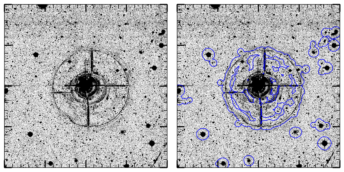
Figure 6: Saturated star masking. The masked regions are contoured in blue against a smoothed cut-out of NGVS $g$-band data. The image size is 4000$\times$4000 pixels, or $\sim$12.5$\times$12.5 arcminutes. The large mask in the centre successfully masks out the LSB ring around the saturated star and we find no detections in its vicinity.

The masked regions were set to zero and this data was used as the input to SExtractor. For this we used a DETECT_THRESH of 6 (see $\S$5.3) and convolved the image with the default filter (a 5$\times$5 pixel Gaussian filter of FWHM 2 pixels). This makes us sensitive to sources with surface brightnesses $\geq\sim$25$g\mu$ for the final DBSCAN run. We disabled de-blending in order to prevent the fragmentation of sources close to the detection threshold as this produced poor masks in their vicinities. We allowed SExtractor to perform its own background and RMS estimates in small meshes of size 64$\times$64 pixels to better detect smaller sources against their local background. All other parameters were left to their defaults. The isophotal radii were then calculated as described in $\S$3.3 for the 29$g\mu$ isophote.

In a minority of cases, the initial SExtractor mask did not cover the full source. This was particularly true for bright galaxies with extended LSB halos and bright unsaturated point sources where the approximate Sérsic fits were inadequate. Requiring a fainter masking isophote did not solve the issue, so we were forced to enlarge the apertures by a factor of 1.5 for these sources (this was determined empirically).

Each mask took approximately 30 minutes to generate. On average, 28 percent of each frame was masked excluding the border regions.

5.2 Sky modelling

We use the source mask as an input to DeepScan’s sky modelling routine. We add to the map by masking sources detected by DBSCAN with the default paramters described in $\S$3.2; this allows sources to masked to well below the sky RMS level. We only do one iteration of the DeepScan detection/masking process as the mask is already quite complete. The sky itself was measured in 500$\times$500 pixels and is median filtered over 3$\times$3 pixels. The large sky-mesh along with the median filtering increases our robustness against bias in the sky measurement due to unmasked LSB haloes. A second advantage is that 500 pixels ($\sim$90$\arcsec$) is large compared to the sources we are searching for so they should not be significantly subtracted with the sky.

5.3 Source detection

The relevant parameters for the segmentation map generation using DBSCAN are the detection threshold, the search radius $\epsilon$ and $\kappa$. Our approach for setting the parameters was to perform empirical tests on a field image (this is an NGVS frame of an area of sky displaced from Virgo where we expect a low density of LSB objects). The detection threshold was set to 0.5 times the RMS ($\sim 27.7g_{\mu}$) because lowering it much further made us sensitive to image artefacts such as background defects. An $\epsilon$ value of 10” ($\sim$50 pixels) was used as this is the smallest aperture that can critically sample an UDG at Virgo distance (UDGs have minimum size of 1.5Kpc van Dokkum et al. (2015) so at 16.5Mpc this is $\sim$20$\arcsec$). With these settings we can expect to detect UDGs with average SB within their effective radii of $\sim 28g_{\mu}$. We ran the field image through the overall pipeline for several values of $\kappa$ and SExtractor detection thresholds (for the mask generation), with results shown in figure 7.

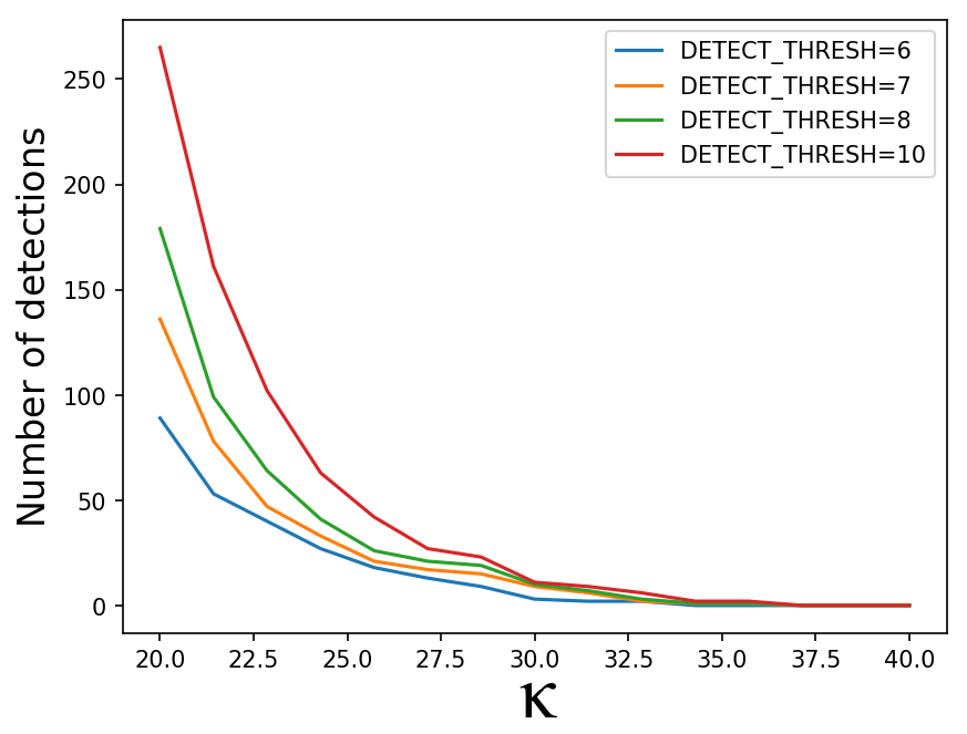
Figure 7: DeepScan parameter tuning. Here we show the effect of varying the SExtractor detection threshold DETECT_THRESH and $\kappa$ parameter on the number of detections on a background NGVS frame. The number of sources detected begins to level off for $\kappa\geq 30$ for each value of DETECT_THRESH.

From the figure, it is clear that the results converge for high values of $\kappa$. We select a value of $\kappa$=32.5 based on this plot by requiring less than 5 detections on the field image. With regards to the SExtractor detection threshold, we were interested in a value that was low enough in order to have a reasonably low number of contaminant objects while being high enough not to partially mask out LSB sources with shredded detections. We adopt a DETECT_THREHSH of 6 to lower the number of contaminant sources. Note that we did not probe lower values than 6 for the masking because this encroaches too far into the LSB regime, with surface brightnesses fainter than $\sim$25 magnitudes per square arcsecond.

There is actually a significant difference in the background RMS level between the frames which makes us sensitive to different surface brightnesses from frame to frame. When we ran all the frames with the same settings as above, we found there was much more contamination of the output sample from spurious sources on some frames compared to others. We therefore normalised the threshold for each frame to the absolute surface brightness corresponding to that which was used on the field image, with settings as above. This is because lowering the threshold (in SNR) for frames with relatively high background RMS increases $\eta$ sufficiently to protect against the spurious detections.

After setting the parameters, DBSCAN was run and took approximately 12 minutes per frame. In total, 67 objects were detected.

5.4 Detection analysis

Each source was assessed visually in order to determine whether it was an astrophysical LSB source or miss-detection. We define miss-detections to encompass data artefacts (such as stellar diffraction rings and satellite trails) and the real LSB component of bright sources that have been inadequately masked. 14 of the raw detections were deemed to be miss-detections, leaving us with a sample of 53 objects. Of the rejected sources, 5 were associated with bright objects, 3 were unmasked stellar halos, 3 were satellite trails, 2 were caused by artefacts from the data stacking procedure and one was an extended LSB bloom caused by a bright source outside the FOV. The rejected sources are shown for clarity in figure 8.

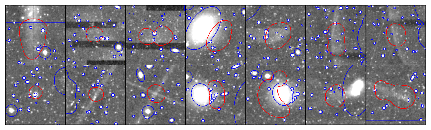
Figure 8: Smoothed $g$-band cut-outs of the rejected detections. The maximum brightness of the dynamic range is approximately 25.5 magnitudes per square arcsecond. The red contour show the dilated segmentation maps produced with DBSCAN and the blue contour traces the mask.

The remaining sources were cross-matched with the VCC (Binggeli et al., 1985), LSBVCC (Davies et al., 2016) and Sabatini et al. (2005) catalogues, using a search radius of 20$\arcsec$ (chosen so large to account for positional uncertainty in other surveys). 23 of the sources had matches, leaving a sample of 30 new LSB galaxies.

We used DeepScan to fit 1D Sérsic profiles to the detections ignoring masked regions. We used the segmap_dilated to estimate elliptical parameters and the centroid positions. 500$\times$500 pixel cut-outs were obtained from the original data, the sky and RMS maps as well as the source mask and dilated segmentation map, centred on these centroids.

The cut-outs were then used as inputs to the 2D Bayesian profile fitting package ProFit, with initial parameter guesses given by the 1D fits. We follow the methodology suggested by the ProFit team, which consists of a three stage fitting process. First, a BFGS gradient decent fit is obtained. The results from this are then used as the initial parameters for a Laplace approximation using the method of Levenberg-Marquardt (LM). Finally, the results are used as the initial guesses for a more robust MCMC fit using the component-wise hit-and-run metropolis (CHARM) algorithm, with 1000 iterations. In the fitting we used a simple Gaussian PSF of FWHM 1$\arcsec$.

The residuals for each fit were judged by-eye to ensure they were reasonable. In general they were, but for 8 of the sources we had to slightly modify the mask in order to get a good fit. Taking the standard deviation of the posterior distributions for each parameter result in uncertainty underestimates, likely because the high-quality of the initial parameter estimates and limited number of iterations mean only a narrow region of parameter space can be explored. To get a more realistic error, the upper and lower range of the posterior distributions were used as the parameter uncertainties.

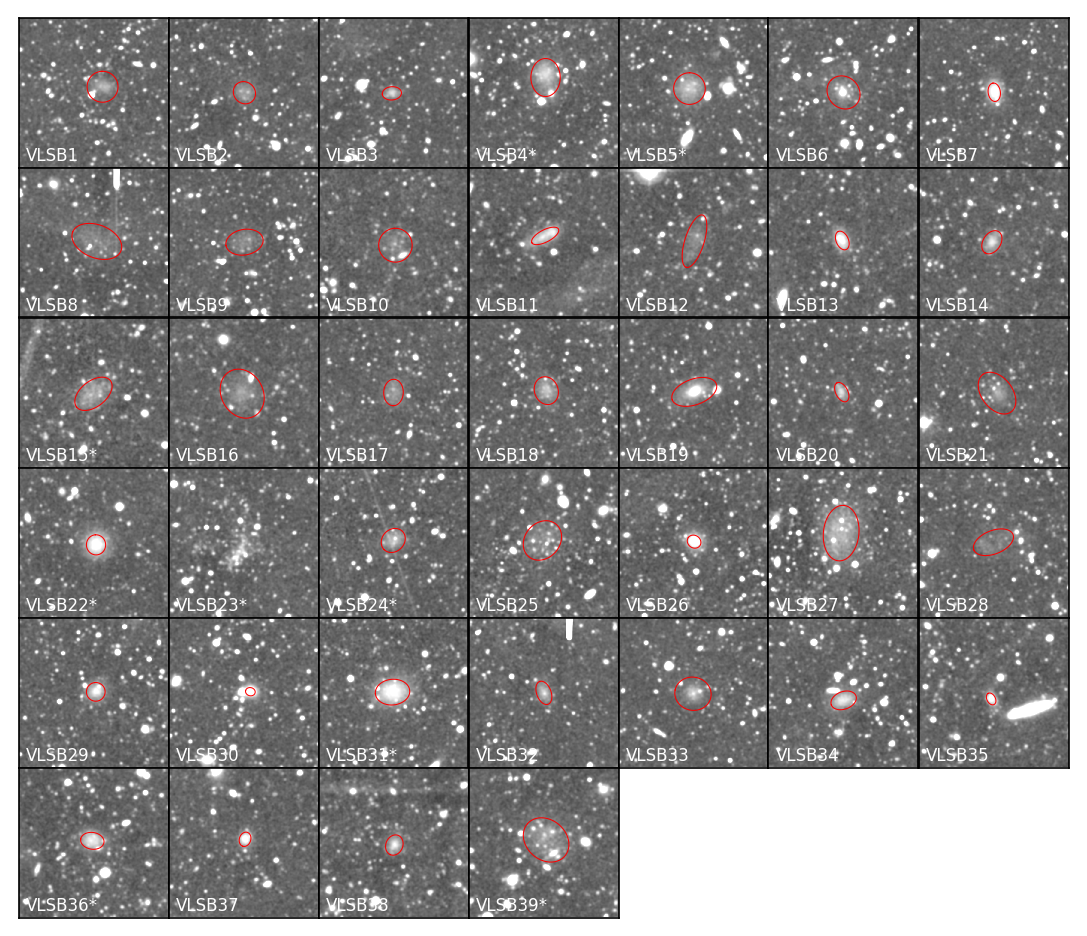
Figure 14: Smoothed $g$-band cut-outs of our new detections. While some of the sample appear reasonably bright, the maximum brightness of the dynamic range is approximately 25.5 magnitudes per square arcsecond, which is close to the faint end limit of detection for the LSBVCC. The red ellipses show the ProFit models out to the effective radii. Sources with an asterisk following their name are also present in the catalogue of Sabatini et al. (2005).

In figure 14 (appendix) we show the cut-outs for our final sample that contains new detections and those that had a match only in the catalogue of Sabatini et al. (2005). We also provide a measurements table for these sources in the appendix. This is done because this catalogue does not cover the whole of Virgo in the same way that the VCC and LSBVCC do. These matches are of genuinely very low surface brightness and are obtained from a different dataset using a matched filter approach, making their re-detection a good coincidence test. We denote the names of galaxies in our final sample that had matches within the Sabatini catalogue with an asterisk after their name. On the figure we also show the elliptical annuli corresponding to the ProFit fits out to the effective radius. Note that the galaxy VLSB23 does not have any measurements due to its highly unusual morphology, an odd over-density of point sources superimposed on a LSB fuzz, and may be worth investigating further.

5.5 Results

We plot the effective radius ($r_{e}$) vs the mean surface brightness within the effective radius ($\langle\mu_{e}\rangle$) based on our ProFit models in figure 9 for the final sample (includes matching Sabatini et al. (2005) sources). On the plot we also show the LSBVCC sample. However, the measurements presented in Davies et al. (2016) are in central surface brightness and exponential scale size units, and all assume a Sérsic index of 1. To try and quantify the uncertainty this introduces on the $r_{e}$ - $\langle\mu_{e}\rangle$ plane, we take their initial results and calculate the relevant parameters using Sérsic indices randomly generated based on our sample ($\langle n\rangle=1.0\pm 0.4$). We also plot the theoretical DBSCAN upper detection boundary assuming $n=1.4$ (i.e. 1$\sigma$ above the mean) which is consistent with our findings.

For context, we also show the selection criteria used by van der Burg et al. (2017) in the figure, who used MegaCam imaging in the search for UDGs around groups and clusters. Further, we plot the sample of Yagi et al. (2016), who obtained a catalogue of LSB galaxies in Coma with deep Subaru-R Suprime-Cam imaging, using their single Sérsic GALFIT (Peng, 2002) fits. These results have been mapped to Virgo $g$-band data by assuming a Virgo distance of 16.5Mpc and a Coma distance of 99Mpc. The Subaru-R to $g$ conversion was done using a fiducial ($g-r$) value of 0.45 (Roediger et al., 2017).

It is clear that the sample in this paper represents an extension of the parameter space explored by other surveys towards the very low surface brightness regime, with $\langle\mu_{e}\rangle>\sim 26.5$. It is perhaps surprising that no larger LSB objects were found and this may be in part due to the initial background subtraction performed on the public NGVS data, which is done over scales of 20$\arcsec$. We are hesitant to draw conclusions from this until we have a more complete sample, and completeness estimates, which we intend to acquire in a follow-up paper.

On the figure we also show the complementary sample, that is the sources that we detected but had matches in the VCC or LSBVCC. Two of these, VCC1331 and VCC1882, have measured effective radii larger than 20” and therefore may warrant reclassification to UDGs from their original classification of dwarf ellipticals.

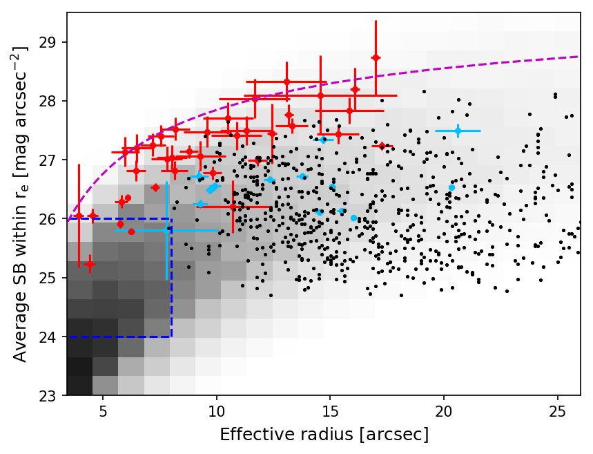
Figure 9: Effective radius vs mean surface brightness within the effective radius for the new sample (red) and the extrapolated LSBVCC data (greyscale heatmap, see text). The light blue points represent the complementary sample. The blue box is the selection criteria used in van der Burg et al. (2017), while the purple dashed line is the theoretical upper limit of detection given our DBSCAN settings. The black dots represent the catalogue of Yagi et al. (2016) projected at Virgo distance.

We measured the ($g-i$) colours of the sample in elliptical apertures out to the effective radii measured in the $g$-band with ProFit. For these measurements, we ignored the masked pixels, the results of which are shown in figure 10. For the $i$-band data we again used the publicly available NGVS data (Ferrarese et al., 2012). We also show measurements from the VCC and LSBVCC obtained by Keenan (2017). The general trend follows the Virgo red-sequence with fainter sources having redder colours and a flattening of the colour towards the faint end, as observed by Roediger et al. (2017). Many of our final sample are consistent with this picture, but there are exceptions. Most noticeably, a collection of sources seems to depart the red sequence at the faint end, in favour of lower $(g-i)$ values. Note that this trend was still observed when recalculating the colours taking into account masked pixels. Two of the sources have unusually high values of ($g-i$). The source with the largest value (VLSB30) may have a biased colour due to its proximity to a star and the second, (VLSB19), seems to be associated with a large nucleated source.

Despite the red colours of the sources, they are generally better-detected in the NGVS $g$-band because fiducially the RMS level of $g$ is $\sim 1.2$ magnitudes per square arcsecond fainter than that of $i$.

We briefly note that 10 of the 14 rejected detections have ($g-i$) colours below the minimum measured from our final sample, as can be seen in the figure. It may therefore be possible to increase the purity of the output automatically by applying a colour selection for future surveys.

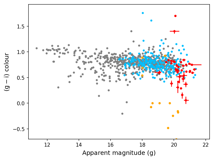
Figure 10: Colour-magnitude diagram for galaxies in the VCC (grey), LSBVCC (blue) and the new sample (red). Many of the new sample are consistent with the Virgo red sequence, but there is a non-negligible sample occupying bluer colour space. The rejected detections are shown in orange.

Figure 11 shows the effective radii, both in units of arcseconds and Kpc (at the Virgo distance of 16.5$\pm$1.1Mpc (Mei et al., 2007)) against the stellar mass calculated using the empirical relation derived by Taylor et al. (2011). The galaxies have a mean (logged) stellar mass of $10^{6.3\pm 0.5}M_{\odot}$, making them fairly less massive than the sample of UDGs presented in van Dokkum et al. (2015), which have a median stellar mass of $6\times 10^{7}M_{\odot}$. Note that if the colours are measured without their source masks in place, the average stellar mass rises only slightly to $10^{6.4\pm 1.0}M_{\odot}$. There is an outlier in the plot that corresponds to VLSB30 which is in proximity to a star. It is likely that the colour has been considerably effected by the star such that the stellar mass estimate may be erroneous.

On the figure we have also plotted estimates of the stellar masses of the Yagi et al. (2016) sample projected at Virgo. Clearly there are several uncertainties in this procedure, but to attempt to get a representative picture we have randomly generated a set of data in which uncertain parameters have been perturbed within their errors, including the original error estimates from the GALFIT models as well as uncertainties in distance and colour (we used $(g-i)=0.7\pm 0.2$ based on figure 10). Our final sample seems to be both smaller in terms of size and also stellar content compared to their sample. It is interesting that some of our sources that matched with the VCC/LSBVCC agree well with the projected distribution from the Yagi sample, as it suggests that a re-inspection of the VCC/LSBVCC may result in the reclassification of some objects to UDGs.

None of the final sample are larger than the 1.5 Kpc lower limit required for UDG classification; there is a notable dearth of large LSBs. Given their sizes and low stellar content, we classify them as ultra-faint dwarfs (UFDs). It could also be that the UDG population is already present in the catalogues of the VCC and LSBVCC but has not been explicitly identified as such; an idea supported by the fact that two of the galaxies in the complementary sample likely meet the UDG criteria. We note that the original NGVS background subtraction over 20” may have the effect of causing our measurements of the sizes of galaxies to be underestimates.

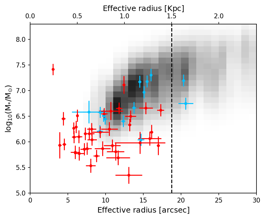
Figure 11: Stellar masses vs effective radius for the final sample (red) and complementary sample (blue) assuming a Virgo distance of 16.5 Mpc. The heat map is the extrapolated data of Yagi et al. (2016) projected at Virgo distance (see text). The black dotted line represents the size of the background estimation kernel in the original data reduction.

6 Discussion and Conclusions

In this paper we have introduced a new software package that we have used to detect low surface brightness features in wide area survey data. The software is capable of measuring the background distribution and producing source masks, currently based on SExtractor catalogues. The major novelty of DeepScan is that it uses a highly efficient implementation of the DBSCAN algorithm to detect LSB features using much larger search radii than has been done before, allowing for the detection of extremely faint extended sources.

As with any detection process, there is a trade-off between completeness and the purity of the output sample. In DeepScan, this is controlled by setting the DBSCAN input parameters: the clustering radius $\epsilon$, the confidence parameter $\kappa$ and the detection threshold thresh. In general, larger values of $\epsilon$ allow for fainter objects to be detected, but using excessively large values may result in source confusion. $\kappa$ must be chosen high enough to protect against spurious detections of e.g. groups of background point sources, but setting it too high may result in unacceptably low completeness.

The purity of the output sample is dependent on the quality of the source mask. Creating a good mask is fairly difficult because of the problems involved in masking out LSB components associated with bright sources that do not adhere to elliptical profiles. Our current approach is to use SExtractor to detect bright sources and mask out to an isophotal radius derived based on fitting a Sérsic profile using outputs from the SExtractor catalogue. This technique is successful in the majority of cases, but is not perfect. In the example application, we masked the LSB components associated with saturated regions using the segmap_dilated produced using DBSCAN. A disadvantage of this is possible source confusion, but is favourable because of its ability to mask large LSB features of arbitrary shape. One promising future approach to creating the source mask could be to use the dilation until convergence approach used by ProFound, which can trace objects of arbitrary shape and thus provide non-parametric source masks.

In the application to the NGVS data, the $\kappa$ value was chosen by measuring the number of objects detected on the frame as a function of $\kappa$ and choosing a value which had a low number of detections. Using such a high value of 32.5 means we have been limited in our capability to fully exploit DBSCAN because of the need to mitigate against contaminant sources in the output sample. Even with such a high value, we still reject 14 out of 67 detections, which consist mainly of satellite trails and unmasked regions associated with bright objects such as saturated stars. It is conceivable that some of these objects may be removed automatically using a colour analysis in future surveys on a larger scale.

Of the remaining 53 sources, 30 do not have matches in either the VCC, LSBVCC or Sabatini catalogues. Keeping the Sabatini sources, we are left with a sample of 39. These measure to have parameter ranges of $26.0\leq\langle\mu_{e}\rangle\leq 28.5g\mu$ and $19\leq m_{g}\leq 21$ following fitting of Sérsic profiles with ProFit. Of this sample, none are large enough to be classified as UDGs and we classify them as UFDs (assuming cluster membership). Our current evidence for cluster membership is that they are reasonably consistent with the colours of other Virgo galaxies, and have angular sizes larger than the optimal selection criterion of $>$3” for Virgo galaxies. Assuming cluster membership, the galaxies have very low stellar masses, with an average of $10^{6.3\pm 0.5}M_{\odot}$.

Comparing our final sample with those from other surveys, we find that we have probed a different region of parameter space, characterised by very low stellar mass estimates and surface brightness. We hypothesise that the dearth of larger detections stems from the initial background subtraction performed on the publicly available NGVS data. Following measurements of two galaxies VCC1331 and VCC1882, it is further hypothesised that some of the UDG population of Virgo may be contained within existing catalogues such as the VCC and LSBVCC.

We have not made any efforts to estimate the completeness of our new sample. In future work we plan to perform a similar analysis on the whole of the NGVS. We aim to quantify the completeness by injecting synthetic sources into the data and measuring what we are able to recover in a similar way to that has been done by van der Burg et al. (2017); only then do we plan on drawing any astrophysical conclusions from our findings. The main conclusions from the experiment we have performed here is that we are able to detect new LSB features in areas that have specifically been searched for them before, which are some of the most diffuse detected in Virgo and reside in a different region in parameter space compared with those in the VCC and LSBVCC catalogues.

Appendix A Statistical limits of DBSCAN

These figures are analagous to figure 2 but for the Sérsic index $n$ and the DBSCAN detection threshold $\kappa$.

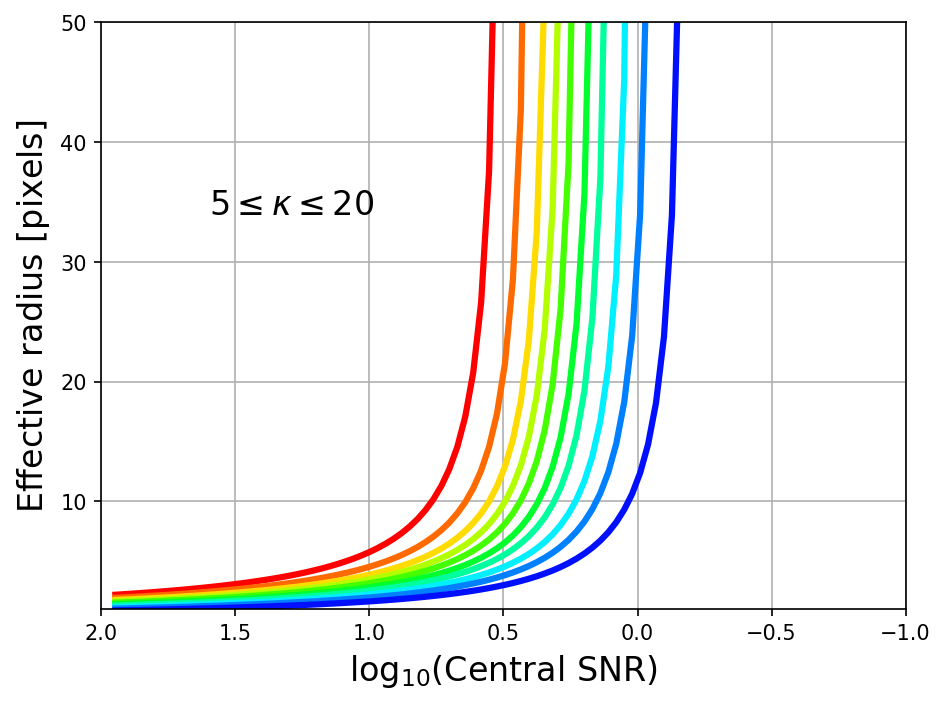
Figure 12: Variation of the limits of detection with $\kappa$, ranging between 5 (blue) and 20 (red), with a colour gradient showing intermediate linearly-spaced values of $\kappa$ increasing with redness. These results were obtained with $\epsilon$=5 pixels, $I_{m}in$=$\sigma_{n}$

.

.

Appendix B Source cut-outs

Smoothed data ($g$-band) cut-outs of our LSBG sample.

Appendix C Source measurements

A table listing measured parameters and their errors for our LSBG sample.

Name	RA [deg]	Dec [deg]	mag ($g$)	$\langle\mu_{e}\rangle$ ($g$)	$r_{e}$ [arcsec]	$n$	$(g-i)$
VLSB1	188.11080	11.62254	20.57 (0.13)	27.47 (0.26)	9.59 (1.04)	1.27 (0.16)	0.47 (0.06)
VLSB2	188.32165	11.62702	20.99 (0.08)	27.25 (0.19)	7.19 (0.55)	0.78 (0.10)	0.61 (0.02)
VLSB3	188.13531	11.70004	21.28 (0.13)	27.13 (0.25)	5.97 (0.62)	1.26 (0.15)	0.66 (0.02)
VLSB4*	188.12484	11.83312	19.64 (0.04)	26.99 (0.08)	11.79 (0.42)	0.94 (0.04)	0.84 (0.01)
VLSB5*	188.31528	11.86882	19.83 (0.05)	26.77 (0.11)	9.81 (0.41)	0.90 (0.06)	0.82 (0.01)
VLSB6	187.74268	11.97468	20.27 (0.09)	27.41 (0.24)	10.87 (1.11)	1.99 (0.07)	0.42 (0.02)
VLSB7	188.29238	12.08603	20.11 (0.03)	25.91 (0.07)	5.75 (0.15)	0.92 (0.07)	0.66 (0.01)
VLSB8	188.07065	12.12576	20.20 (0.08)	28.20 (0.37)	16.08 (0.20)	0.60 (1.11)	0.63 (0.05)
VLSB9	187.94944	12.30602	20.74 (0.15)	28.04 (0.33)	11.66 (1.57)	0.74 (0.16)	0.37 (0.06)
VLSB10	188.72908	11.60686	20.63 (0.13)	27.70 (0.27)	10.50 (1.11)	0.74 (0.16)	0.85 (0.03)
VLSB11	188.78022	11.65995	20.24 (0.06)	27.06 (0.25)	9.28 (1.10)	0.62 (0.06)	0.64 (0.02)
VLSB12	189.01353	11.71026	20.62 (0.11)	28.74 (0.64)	16.98 (0.21)	0.58 (1.15)	0.54 (0.08)
VLSB13	189.22741	11.84436	20.44 (0.02)	26.36 (0.05)	6.10 (0.12)	0.83 (0.04)	0.80 (0.01)
VLSB14	188.89157	11.91654	20.58 (0.09)	27.02 (0.21)	7.81 (0.68)	1.21 (0.12)	0.73 (0.01)
VLSB15*	189.07497	11.95334	19.96 (0.06)	27.58 (0.13)	13.31 (0.71)	0.73 (0.08)	0.82 (0.01)
VLSB16	189.39290	12.10761	19.83 (0.09)	27.83 (0.23)	15.84 (1.52)	0.97 (0.09)	0.39 (0.06)
VLSB17	190.24144	11.60283	20.97 (0.09)	27.52 (0.19)	8.19 (0.63)	0.67 (0.10)	0.77 (0.02)
VLSB18	189.60967	11.65298	20.44 (0.05)	27.14 (0.11)	8.78 (0.41)	1.01 (0.07)	0.29 (0.02)
VLSB19	190.01774	11.83603	20.03 (0.22)	27.44 (0.51)	12.44 (0.20)	1.33 (1.63)	1.40 (0.05)
VLSB20	189.68450	11.94874	21.16 (0.11)	27.20 (0.24)	6.47 (0.67)	1.13 (0.14)	0.59 (0.02)
VLSB21	190.25336	12.03853	20.34 (0.28)	28.10 (0.68)	14.55 (3.37)	1.32 (0.25)	0.52 (0.13)
VLSB22*	189.98940	12.11310	19.82 (0.02)	25.78 (0.05)	6.24 (0.14)	0.78 (0.03)	0.78 (0.00)
VLSB23*	189.75714	12.20416	–	–	–	–	–
VLSB24*	189.69605	12.23770	20.52 (0.09)	27.04 (0.21)	8.02 (0.66)	1.02 (0.15)	0.16 (0.07)
VLSB25	190.25519	12.28037	20.17 (0.04)	27.76 (0.18)	13.18 (0.19)	0.53 (1.08)	0.73 (0.03)
VLSB26	191.04250	11.57866	20.02 (0.10)	25.23 (0.16)	4.40 (0.27)	1.88 (0.34)	0.81 (0.02)
VLSB27	190.82000	11.62940	19.05 (0.03)	27.24 (0.07)	17.28 (0.46)	0.63 (0.03)	0.59 (0.01)
VLSB28	191.27329	11.66796	20.75 (0.18)	28.32 (0.34)	13.06 (1.79)	0.34 (0.07)	0.06 (0.07)
VLSB29	190.69944	11.69863	20.48 (0.05)	26.29 (0.12)	5.80 (0.28)	1.15 (0.08)	0.64 (0.02)
VLSB30	191.10218	11.94348	20.09 (0.03)	24.48 (0.14)	3.03 (0.18)	2.50 (0.00)	1.70 (0.00)
VLSB31*	191.31792	12.24813	19.08 (0.32)	26.20 (0.44)	10.70 (1.60)	1.44 (0.79)	0.60 (0.03)
VLSB32	190.89820	12.32410	21.02 (0.07)	27.40 (0.18)	7.55 (0.58)	1.03 (0.14)	0.63 (0.02)
VLSB33	191.07622	12.33591	20.23 (0.10)	27.49 (0.24)	11.31 (1.15)	1.86 (0.16)	0.31 (0.11)
VLSB34	190.55282	12.37594	20.27 (0.04)	26.82 (0.16)	8.15 (0.59)	0.92 (0.06)	0.71 (0.01)
VLSB35	192.03936	11.59721	21.14 (0.29)	26.05 (0.88)	3.92 (0.23)	0.89 (1.19)	0.75 (0.01)
VLSB36*	191.69418	11.65545	20.22 (0.03)	26.53 (0.07)	7.29 (0.21)	0.75 (0.05)	0.61 (0.01)
VLSB37	192.28541	11.91996	20.78 (0.06)	26.05 (0.12)	4.53 (0.25)	1.14 (0.12)	0.62 (0.01)
VLSB38	191.70495	11.94819	20.76 (0.08)	26.81 (0.18)	6.46 (0.43)	1.40 (0.11)	0.75 (0.01)
VLSB39*	191.70132	12.19595	19.51 (0.08)	27.43 (0.16)	15.34 (0.91)	0.71 (0.09)	0.80 (0.01)

References

- Aihara et al. (2017) Aihara H., et al., 2017, preprint, (arXiv:1702.08449)
- Akhlaghi & Ichikawa (2015) Akhlaghi M., Ichikawa T., 2015, The Astrophysical Journal Supplement Series, 220, 1
- Amorisco & Loeb (2016) Amorisco N. C., Loeb A., 2016, Monthly Notices of the Royal Astronomical Society: Letters, 459, L51
- Beasley & Trujillo (2016) Beasley M. A., Trujillo I., 2016, The Astrophysical Journal, 830, 23
- Berry (2015) Berry D. S., 2015, Astronomy and Computing, 10, 22
- Bertin & Arnouts (1996) Bertin E., Arnouts S., 1996, Astronomy and Astrophysics Supplement Series, 117, 393
- Bhattacharya et al. (2017) Bhattacharya S., Mahulkar V., Pandaokar S., Singh P., 2017, Astronomy and Computing, 18, 1
- Binggeli et al. (1985) Binggeli B., Sandage A., Tammann G. A., 1985, The Astronomical Journal, 90, 1681
- Blanton et al. (2011) Blanton M. R., Kazin E., Muna D., Weaver B. A., Price-Whelan A., 2011, AJ, 142, 31
- Butler-Yeoman et al. (2016) Butler-Yeoman T., Frean M., Hollitt C. P., Hogg D. W., Johnston-Hollitt M., 2016, preprint, (arXiv:1601.00266)
- Collins et al. (2013) Collins M. L. M., et al., 2013, The Astrophysical Journal, 768, 172
- Cooper et al. (2010) Cooper A. P., et al., 2010, MNRAS, 406, 744
- Davies et al. (2016) Davies J. I., Davies L. J. M., Keenan O. C., 2016, MNRAS, 456, 1607
- Di Cintio et al. (2017) Di Cintio A., Brook C. B., Dutton A. A., Macciò A. V., Obreja A., Dekel A., 2017, MNRAS, 466, L1
- Disney (1976) Disney M., 1976, Nature, 260, 643
- Driver et al. (2016) Driver S. P., et al., 2016, The Astrophysical Journal, pp 1–21
- Edge et al. (2013) Edge A., Sutherland W., Kuijken K., Driver S., McMahon R., Eales S., Emerson J. P., 2013, The Messenger, 154, 32
- Ester et al. (1996) Ester M., Kriegel H.-P., Sander J., Xu X., 1996. AAAI Press, pp 226–231
- Ferrarese et al. (2012) Ferrarese L., et al., 2012, The Astrophysical Journal Supplement Series, 200, 4
- Fliri & Trujillo (2015) Fliri J., Trujillo I., 2015, Monthly Notices of the Royal Astronomical Society, 456, 1359
- Graham & Driver (2005) Graham A. W., Driver S. P., 2005, Publications of the Astronomical Society of Australia, 22, 118
- Greco et al. (2017) Greco J. P., et al., 2017, preprint, (arXiv:1709.04474)
- Guttman (1984) Guttman A., 1984, Proceedings of the 1984 ACM SIGMOD international conference on Management of data - SIGMOD ’84, p. 47
- Janssens et al. (2017) Janssens S., Abraham R., Brodie J., Forbes D., Romanowsky A. J., van Dokkum P., 2017, The Astrophysical Journal Letters, 839, L17
- Javanmardi et al. (2016) Javanmardi B., et al., 2016, Astronomy & Astrophysics, 588, A89
- Kambas et al. (2000) Kambas A., Davies J., Smith R., Bianchi S., Haynes J., 2000, The Astronomical Journal, 120, 1316
- Keenan (2017) Keenan O. C., 2017, PhD thesis, School of Physics & Astronomy, Cardiff University, The Parade, Cardiff, CF24 3AA, UK
- Kochoska et al. (2017) Kochoska A., Mowlavi N., Prša A., Lecoeur-Taïbi I., Holl B., Rimoldini L., Süveges M., Eyer L., 2017, A&A, 602, A110
- Koda et al. (2015) Koda J., Yagi M., Yamanoi H., Komiyama Y., 2015, The Astrophysical Journal, 807, L2
- McGaugh (1996) McGaugh S. S., 1996, Monthly Notices of the Royal Astronomical Society, 280, 337
- Mei et al. (2007) Mei S., et al., 2007, The Astrophysical Journal, 655, 144
- Mihos et al. (2005) Mihos J. C., Harding P., Feldmeier J., Morrison H., 2005, The Astrophysical Journal Letters, 631, L41
- Mihos et al. (2015) Mihos J. C., et al., 2015, The Astrophysical Journal Letters, 809, L21
- Mihos et al. (2017) Mihos J. C., Harding P., Feldmeier J. J., Rudick C., Janowiecki S., Morrison H., Slater C., Watkins A., 2017, The Astrophysical Journal, 834, 16
- Mowla et al. (2017) Mowla L., van Dokkum P., Merritt A., Abraham R., Yagi M., Koda J., 2017, ApJ, 851, 27
- Müller et al. (2017) Müller O., Jerjen H., Binggeli B., 2017, A&A, 597, A7
- Muñoz et al. (2015) Muñoz R. P., et al., 2015, The Astrophysical Journal, 813, L15
- Peng (2002) Peng C., 2002, Astronomy, pp 733–759
- Robotham et al. (2017) Robotham A. S. G., Taranu D. S., Tobar R., Moffett A., Driver S. P., 2017, MNRAS, 466, 1513
- Robotham et al. (2018) Robotham A. S. G., Davies L. J. M., Driver S. P., Koushan S., Taranu D. S., Casura S., Liske J., 2018, 24, 1
- Roediger et al. (2017) Roediger J. C., et al., 2017, The Astrophysical Journal, 836, 120
- Román & Trujillo (2017) Román J., Trujillo I., 2017, MNRAS, 468, 4039
- Sabatini et al. (2005) Sabatini S., Davies J., Van Driel W., Baes M., Roberts S., Smith R., Linder S., O’Neil K., 2005, Monthly Notices of the Royal Astronomical Society, 357, 819
- Shull et al. (2012) Shull J. M., Smith B. D., Danforth C. W., 2012, The Astrophysical Journal, 759, 23
- Sifón et al. (2018) Sifón C., van der Burg R. F. J., Hoekstra H., Muzzin A., Herbonnet R., 2018, MNRAS, 473, 3747
- Slater et al. (2009) Slater C. T., Harding P., Mihos J. C., 2009, PASP, 121, 1267
- Taylor et al. (2011) Taylor E. N., et al., 2011, Monthly Notices of the Royal Astronomical Society, 418, 1587
- Teeninga et al. (2016) Teeninga P., Moschini U., Trager S. C., Wilkinson M. H., 2016, Mathematical Morphology - Theory and Applications, 1, 100
- Venhola et al. (2017) Venhola A., et al., 2017, A&A, 608, A142
- Williams et al. (1994) Williams J. P., de Geus E. J., Blitz L., 1994, The Astrophysical Journal, 428, 693
- Yagi et al. (2016) Yagi M., Koda J., Komiyama Y., Yamanoi H., 2016, The Astrophysical Journal Supplement Series, 225, 11
- Zheng et al. (2015) Zheng C., Pulido J., Thorman P., Hamann B., 2015, Monthly Notices of the Royal Astronomical Society, 451, 4445
- de Jong et al. (2015) de Jong J. T. A., et al., 2015, A&A, 582, A62
- van Dokkum et al. (2015) van Dokkum P. G., Abraham R., Merritt A., Zhang J., Geha M., Conroy C., 2015, The Astrophysical Journal, 798, L45
- van Dokkum et al. (2017) van Dokkum P., et al., 2017, ApJ, 844, L11
- van der Burg et al. (2016) van der Burg R. F. J., Muzzin A., Hoekstra H., 2016, Astronomy & Astrophysics, 590, A20
- van der Burg et al. (2017) van der Burg R. F. J., et al., 2017, A&A, 607, A79