Long-time energy analysis of extended RKN integrators for muti-frequency highly oscillatory Hamiltonian systems

Abstract

In this paper, we study the long-time near conservation of the total and oscillatory energies for extended RKN (ERKN) integrators when applied to muti-frequency highly oscillatory Hamiltonian systems. We consider one-stage explicit symmetric integrators and show their long-time behaviour of numerical energy conservations by using modulated multi-frequency Fourier expansions. Numerical experiments are carried out and the numerical results demonstrate the remarkable long-time near conservation of the energies for the ERKN integrators and support our theoretical analysis presented in this paper.

Keywords: Long-time energy conservation Modulated Fourier expansions Muti-frequencies highly oscillatory systems Hamiltonian systems Extended RKN integrators

MSC:65P10 65L05

1 Introduction

The study of numerical energy preservation is an important aspect of numerical analysis in the sense of structure-preserving algorithms when applied to Hamiltonian systems. This paper is devoted to muti-frequency highly oscillatory Hamiltonian systems with the following Hamiltonian function

$$\begin{array}[c]{ll}H(q,p)&=\dfrac{1}{2}\textstyle\sum\limits_{j=0}^{l}\Big{(}\left\|p_{j}\right\|^{2}+\dfrac{\lambda_{j}^{2}}{\epsilon^{2}}\left\|q_{j}\right\|^{2}\Big{)}+U(q),\end{array}$$ (1)

where $q=(q_{0},q_{1},\ldots,q_{l}),\ p=(p_{0},p_{1},\ldots,p_{l})$ with $q_{j},\ p_{j}\in\mathbb{R}^{d_{j}}$, $\lambda_{0}=0$ and $\lambda_{j}\geq 1$ for $j\geq 1$ are distinct real numbers , $\epsilon$ is a small positive parameter, and $U(q)$ is a smooth potential function. We pay attention to the muti-frequency case where $l>1.$ As is known, this system has the oscillatory energy of the $j$th frequency as

$$I_{j}(q,p)=\dfrac{1}{2}\Big{(}\left\|p_{j}\right\|^{2}+\dfrac{\lambda_{j}^{2}}{\epsilon^{2}}\left\|q_{j}\right\|^{2}\Big{)},$$

and its total oscillatory energy is given by $I(q,p)=\sum\limits_{j=1}^{l}I_{j}(q,p).$ Letting

$$\lambda=(\lambda_{1},\ldots,\lambda_{l}),\quad k=(k_{1},\ldots,k_{l}),\quad k\cdot\lambda=k_{1}\lambda_{1}+\cdots+k_{l}\lambda_{l},$$

and denoting the resonance module by

$$\mathcal{M}=\{k\in\mathbb{Z}^{l}:\ k\cdot\lambda=0\},$$ (2)

it follows from the analysis in [1] that the quantities

$$I_{\mu}(q,p)=\sum\limits_{j=1}^{l}\frac{\mu_{j}}{\lambda_{j}}I_{j}(q,p)\quad\mathrm{with}\ \mu\ \mathrm{orthogonal\ to}\ \mathcal{M}$$

are approximately preserved under a diophantine non-resonance condition outside $\mathcal{M}$. Here, it is clear that $I_{\lambda}=I(q,p)$.

This kind of muti-frequency highly oscillatory systems often arises in various fields such as applied mathematics, molecular biology, astronomy, and classical mechanics (see, e.g. [14, 16, 25, 30]). In recent years, many effective numerical methods have been developed and see, e.g. [9, 11, 15, 18, 22, 23, 26] as well as the references contained therein. In [29], the authors formulated a kind of trigonometric integrators called as extended Runge–Kutta–Nyström (ERKN) integrators for solving muti-frequency highly oscillatory systems. Some important properties of these integrators were further studied in [27, 28, 30]. Very recently, the long-time energy conservation of ERKN integrators for highly oscillatory Hamiltonian systems with one frequency was researched in [24]. On the basis of this work, this paper is devoted to the numerical energy analysis of ERKN integrators for muti-frequency highly oscillatory Hamiltonian systems.

For the analysis of energy preservation, modulated Fourier expansions are an elementary and useful analytical tool. It was firstly developed in [10] and then was used as an important mathematical tool in studying the long-time behaviour of numerical methods for differential equations (see, e.g. [2, 3, 4, 5, 6, 7, 8, 12, 13, 17, 19, 20, 21, 24]). The long-time analysis of some trigonometric integrators for muti-frequency oscillatory Hamiltonian systems has been given in [6]. In this paper we extend the long-time energy preservation results of [6, 24] to the ERKN integrators for multi-frequency cases. As is known, resonance frequencies may exist for multi-frequency oscillatory Hamiltonian systems. Hence, compared with the analysis of one-frequency case in [24], a new and important aspect of muti-frequency case is possible resonance among the frequencies, which is similar to the analysis made in [6].

The remainder of this paper is organised as follows. In Section 2, we briefly summarise ERKN integrators for the muti-frequency Hamiltonian systems (1) and present some preliminaries. The modulated Fourier expansion of ERKN integrators are derived and analysed in Section 3 and two almost-invariants of the modulated Fourier expansions are studied in Section 4. Then Section 5 presents the main result concerning the long-time near energy conservation. Numerical experiments are accompanied in Section 6. The last section is concerned with the conclusions of this paper.

2 Preliminaries

2.1 ERKN integrators

Rewrite the highly oscillatory system (1) as a system of second-order differential equations

$$q^{\prime\prime}=-\Omega^{2}q+g(q),\qquad q(0)=q^{0},\ \ p(0)=p^{0},$$ (3)

where $\Omega=\textmd{diag}(\omega_{0}I_{d_{0}},\omega_{1}I_{d_{1}},\ldots,\omega_{l}I_{d_{l}})$ with $\omega_{j}=\lambda_{j}/\epsilon$ and $g(q)=-\nabla U(q).$ A kind of trigonometric integrators called as ERKN integrators has been developed (see, e.g. [29]), and the one-stage ERKN explicit scheme will be discussed in detail in this paper.

Definition 1

(See [29]) A one-stage explicit ERKN integrator for (3) is defined by

$$\begin{array}[c]{ll}Q^{n+c_{1}}&=\phi_{0}(c_{1}^{2}V)q^{n}+hc_{1}\phi_{1}(c_{1}^{2}V)p^{n},\\ q^{n+1}&=\phi_{0}(V)q^{n}+h\phi_{1}(V)p^{n}+h^{2}\bar{b}_{1}(V)g(Q^{n+c_{1}}),\\ p^{n+1}&=-h\Omega^{2}\phi_{1}(V)q^{n}+\phi_{0}(V)p^{n}+h\textstyle b_{1}(V)g(Q^{n+c_{1}}),\end{array}$$ (4)

where $h$ is a stepsize, $c_{1}$ is real constant satisfying $0\leq c_{1}\leq 1$ , $b_{1}(V)$ and $\bar{b}_{1}(V)$ are matrix-valued and uniformly bounded functions of $V\equiv h^{2}\Omega^{2}$, and

$$\phi_{j}(V):=\sum\limits_{k=0}^{\infty}\dfrac{(-1)^{k}V^{k}}{(2k+j)!},\qquad j=0,1,\ldots.$$ (5)

The following three results of ERKN integrators will be useful in this paper.

Theorem 1

(See [29, 30]) The one-stage explicit ERKN integrator (4) is of order two if and only if

$$\begin{array}[c]{l}b_{1}(V)=\phi_{1}(V)+\mathcal{O}(h^{2}),\ \ c_{1}b_{1}(V)=\phi_{2}(V)+\mathcal{O}(h),\ \ \bar{b}_{1}(V)=\phi_{2}(V)+\mathcal{O}(h).\end{array}$$

Theorem 2

(See [30]) If and only if

$$c_{1}=1/2,\ \bar{b}_{1}(V)=\phi_{1}(V)b_{1}(V)-\phi_{0}(V)\bar{b}_{1}(V),\ \phi_{0}(c_{1}^{2}V)\bar{b}_{1}(V)=c_{1}\phi_{1}(c_{1}^{2}V)b_{1}(V),$$ (6)

then the one-stage explicit ERKN integrator (4) is symmetric.

Theorem 3

(See [30]) If there exists a real number $d_{1}$ such that

$$\phi_{0}(V)b_{1}(V)+V\phi_{1}(V)\bar{b}_{1}(V)=d_{1}\phi_{0}(c_{1}^{2}V),\ \ \ d_{1}\in\mathbb{R},$$

$$\phi_{1}(V)b_{1}(V)-\phi_{0}(V)\bar{b}_{1}(V)=c_{1}d_{1}\phi_{1}(c_{1}^{2}V),$$

then the one-stage explicit ERKN integrator (4) is symplectic.

2.2 Notations

Let $V=h^{2}\Omega^{2}$. It follows from (5) that

$$\phi_{0}(V)=\cos(h\Omega),\qquad\phi_{1}(V)=\textmd{sinc}(h\Omega):=(h\Omega)^{-1}\sin(h\Omega).$$

Throughout this paper, we use the notations $\bar{b}_{1}(h\Omega)$ and $b_{1}(h\Omega)$ to denote the coefficients appearing in the ERKN method (4). Moreover, we also adopt the following notations which appeared in [6]:

$$\omega=(\omega_{1},\ldots,\omega_{l}),\quad\langle j\rangle=(0,\ldots,1,\ldots,0),\quad|k|=|k_{1}|+\cdots+|k_{l}|.$$

For the resonance module (2), we let $\mathcal{K}$ be a set of representatives of the equivalence classes in $\mathbb{Z}^{l}\backslash\mathcal{M}$ which are chosen such that for each $k\in\mathcal{K}$ the sum $|k|$ is minimal in the equivalence class $[k]=k+\mathcal{M},$ and that with $k\in\mathcal{K}$, also $-k\in\mathcal{K}.$ We denote, for the positive integer $N$,

$$\mathcal{N}=\{k\in\mathcal{K}:\ |k|\leq N\},\ \ \ \ \ \mathcal{N}^{*}=\mathcal{N}\backslash\{(0,\ldots,0)\}.$$ (7)

In this paper, we use the following operator which has been defined in [14]

$$\mathcal{L}(hD): =\mathrm{e}^{hD}-2\cos(h\Omega)+\mathrm{e}^{-hD}=2\big{(}\cos(\mathrm{i}hD)-\cos(h\Omega)\big{)}$$

$$=4\sin\big{(}\frac{1}{2}h\Omega+\frac{1}{2}\mathrm{i}hD\big{)}\sin\big{(}\frac{1}{2}h\Omega-\frac{1}{2}\mathrm{i}hD\big{)},$$

where $D$ is the differential operator. It is easy to verify that $(hD)^{m}x(t)=h^{m}x^{(m)}(t)$ for $m=0,1,\ldots,$ and $\mathrm{e}^{hD}x(t)=x(t+h).$

We consider the application of such an operator to functions of the form $\mathrm{e}^{\mathrm{i}(k\cdot\omega)t}.$ By Leibniz’ rule of calculus, one has

$$(hD)^{m}\mathrm{e}^{\mathrm{i}(k\cdot\omega)t}z(t)=\mathrm{e}^{\mathrm{i}(k\cdot\omega)t}(hD+\mathrm{i}(k\cdot\omega)h)^{m}z(t),$$

which yields $f(hD)\mathrm{e}^{\mathrm{i}(k\cdot\omega)t}z(t)=\mathrm{e}^{\mathrm{i}(k\cdot\omega)t}f(hD+\mathrm{i}(k\cdot\omega)h)z(t),$ where

$$f(hD+\mathrm{i}(k\cdot\omega)h)z(t)=\sum\limits_{m=0}^{\infty}\frac{f^{(m)}(\mathrm{i}(k\cdot\omega)h)}{m!}h^{m}z^{(m)}(t).$$

Furthermore, we have the following proposition of the operator.

Proposition 1

The Taylor expansions of $\mathcal{L}(hD)$ and $\mathcal{L}(hD+\mathrm{i}(k\cdot\omega)t)$ are

$$\mathcal{L}(hD)= 4\sin^{2}(h\Omega/2)-I(\mathrm{i}hD)^{2}+\ldots,$$

$$\mathcal{L}(hD+\mathrm{i}(k\cdot\omega)h)= \big{(}2\cos((k\cdot\omega)h)I-2\cos(h\Omega)\big{)}+2\sin((k\cdot\omega)h)I(\mathrm{i}hD)$$

$$-\cos((k\cdot\omega)h)I(\mathrm{i}hD)^{2}+\ldots.$$

3 Modulated Fourier expansion of the integrators

Before presenting the analysis of long-time conservation, we make the following assumptions. The first four assumptions have been considered in [6].

Assumption 1

$\bullet$ The initial values are assumed to satisfy

$$\frac{1}{2}\left\|p^{0}\right\|^{2}+\frac{1}{2}\left\|\Omega q^{0}\right\|^{2}\leq E.$$

$\bullet$ It is assumed that the numerical solution $Q^{n+c_{1}}$ stays in a compact set on which the potential $U$ is smooth.

$\bullet$ A lower bound is posed for the stepsize $h/\epsilon\geq c_{0}>0.$

$\bullet$ Assume that the following numerical non-resonance condition holds

$$|\sin(\frac{h}{2\epsilon}(k\cdot\lambda))|\geq c\sqrt{h}\ \ \mathrm{for}\ \ k\in\mathbb{Z}^{l}\backslash\mathcal{M}\ \ \mathrm{with}\ \ |k|\leq N$$ (8)

for some $N\geq 2$ and $c>0$. In this paper, the $\mathcal{N}$ given in (7) is defined for this $N$.

$\bullet$ The ERKN integrators are required to satisfy the symmetry conditions (LABEL:sym_cond). Moreover, it is assumed that

$$|b_{1}(h\omega_{j})|\leq C_{2}|\textmd{sinc}(h\omega_{j}/2)|,$$

for $j=1,\ldots,l.$

Remark 1

It is clear that we consider the numerical non-resonance condition (8) in the analysis of this paper, which is the same as that in [6]. We also noted that the long-term analysis of some integrators for oscillatory systems under minimal non-resonance conditions has recently been presented in [4]. The long-time analysis of ERKN integrators under minimal non-resonance conditions will be our next work in the near future.

We will establish a modulated Fourier expansion for the ERKN integrators by the following theorem. It is the multi-frequency version of [24]. Its proof follows the lines of the proof of the corresponding theorem given in [24] but with rather obvious adaptations. In the proof of this theorem, we just briefly highlight the main differences and ignore the same derivations for brevity.

Theorem 4

Suppose that Assumption 1 is true. The ERKN integrator (4) admits the expansions

$$q^{n}=\zeta(t)+\sum\limits_{k\in\mathcal{N}^{*}}\mathrm{e}^{\mathrm{i}(k\cdot\omega)t}\zeta^{k}(t)+R_{h,N}(t),$$

$$p^{n}=\eta(t)+\sum\limits_{k\in\mathcal{N}^{*}}\mathrm{e}^{\mathrm{i}(k\cdot\omega)t}\eta^{k}(t)+S_{h,N}(t),$$

for $0\leq t=nh\leq T$. The remainder terms are bounded by

$$R_{h,N}(t)=\mathcal{O}(th^{N-1}),\ \ \ \ S_{h,N}(t)=\mathcal{O}(th^{N-1}),$$ (9)

and the coefficient functions as well as all their derivatives are bounded by

$$\begin{array}[c]{rll}&\zeta_{0}(t)=\mathcal{O}(1),&\eta_{0}(t)=\mathcal{O}(1),\\ &\zeta_{j}(t)=\mathcal{O}\Big{(}\frac{h^{2}\bar{b}_{1}(h\omega_{j})}{\sin^{2}(\frac{1}{2}h\omega_{j})}\Big{)}=\mathcal{O}(h),&\eta_{j}(t)=\mathcal{O}\Big{(}\frac{h^{2}b_{1}(h\omega_{j})}{\sin^{2}(\frac{1}{2}h\omega_{j})}\Big{)}=\mathcal{O}(h),\\ &\dot{\zeta}_{j}^{\pm\langle j\rangle}(t)=\mathcal{O}\Big{(}\frac{h^{2}\bar{b}_{1}(h\omega_{j})}{\sin(\pm\omega_{j}h)}\Big{)}=\mathcal{O}(h^{3/2}),&\dot{\eta}_{j}^{\pm\langle j\rangle}(t)=\mathcal{O}\Big{(}\frac{h^{2}b_{1}(h\omega_{j})}{\sin(\pm\omega_{j}h)}\Big{)}=\mathcal{O}(h^{3/2}),\\ &\zeta_{j}^{\pm\langle j\rangle}(t)=\mathcal{O}(\epsilon),&\eta_{j}^{\pm\langle j\rangle}(t)=\mathcal{O}(1),\\ &\zeta_{0}^{k}(t)=\mathcal{O}\Big{(}h\epsilon^{|k|}\Big{)},&\eta_{0}^{k}(t)=\mathcal{O}\Big{(}h\epsilon^{|k|}\Big{)},\ \ k\in\mathcal{N}^{*},\\ &\zeta_{j}^{k}(t)=\mathcal{O}\Big{(}h\epsilon^{|k|}\bar{b}_{1}(h\omega_{j})\Big{)}=\mathcal{O}\Big{(}h\epsilon^{|k|}\Big{)},&\eta_{j}^{k}(t)=\mathcal{O}\Big{(}h\epsilon^{|k|}b_{1}(h\omega_{j})\Big{)}=\mathcal{O}\Big{(}h\epsilon^{|k|}\Big{)},\\ &&\qquad\qquad\qquad\qquad\qquad\qquad k\neq\pm\langle j\rangle,\end{array}$$ (10)

for $j=1,\ldots,l$. Moreover, we have $\zeta^{-k}=\overline{\zeta^{k}}$ and $\eta^{-k}=\overline{\eta^{k}}$. The constants symbolised by the notation are independent of $h$ and $\omega$, but depend on $E,\ N,\ c_{0}$ and $T$.

Proof. We will prove that there exist two functions

$$q_{h}(t)=\zeta(t)+\sum\limits_{k\in\mathcal{N}^{*}}\mathrm{e}^{\mathrm{i}(k\cdot\omega)t}\zeta^{k}(t),\ \ \ \ p_{h}(t)=\eta(t)+\sum\limits_{k\in\mathcal{N}^{*}}\mathrm{e}^{\mathrm{i}(k\cdot\omega)t}\eta^{k}(t)$$ (11)

with smooth coefficients $\zeta,\ \zeta^{k},\ \eta,\ \eta^{k}$, such that, for $t=nh$,

$$q^{n}=q_{h}(t)+\mathcal{O}(h^{N}),\ \ \ \ p^{n}=p_{h}(t)+\mathcal{O}(h^{N}).$$

Construction of the coefficients functions.

$\bullet$ For the first term of (4), we look for the function

$$q^{n+\frac{1}{2}}:=\tilde{q}_{h}(t+\frac{h}{2})=\xi(t+\frac{h}{2})+\sum\limits_{k\in\mathcal{N}^{*}}\mathrm{e}^{\mathrm{i}(k\cdot\omega)t}\xi^{k}(t+\frac{h}{2})$$ (12)

for $Q^{n+\frac{1}{2}}$ in the numerical integrator (4). Inserting (11) and (12) into the first term of (4) and comparing the coefficients of $\mathrm{e}^{\mathrm{i}(k\cdot\omega)t}$, one gets

$$\xi(t+\frac{h}{2})=\cos(\frac{1}{2}h\Omega)\zeta(t)+\frac{1}{2}h\mathrm{sinc}(\frac{1}{2}h\Omega)\eta(t),$$

$$\xi^{k}(t+\frac{h}{2})=\cos(\frac{1}{2}h\Omega)\zeta^{k}(t)+\frac{1}{2}h\mathrm{sinc}(\frac{1}{2}h\Omega)\eta^{k}(t).$$

$\bullet$ For the second term of (4), by the symmetry of the integrator, we obtain

$$q^{n+1}-2\cos(h\Omega)q^{n}+q^{n-1}=h^{2}\bar{b}_{1}(h\Omega)\big{[}g(q^{n+\frac{1}{2}})+g(q^{n-\frac{1}{2}})\big{]},$$ (13)

where $q^{n-\frac{1}{2}}$ is defined by $q^{n-\frac{1}{2}}:=\tilde{q}_{h}(t-\frac{h}{2})=\xi(t-\frac{h}{2})+\sum\limits_{k\in\mathcal{N}^{*}}\mathrm{e}^{\mathrm{i}(k\cdot\omega)t}\xi^{k}(t-\frac{h}{2})$ with

$$\xi(t-\frac{h}{2})=\cos(\frac{1}{2}h\Omega)\zeta(t)-\frac{1}{2}h\mathrm{sinc}(\frac{1}{2}h\Omega)\eta(t),$$

$$\xi^{k}(t-\frac{h}{2})=\cos(\frac{1}{2}h\Omega)\zeta^{k}(t)-\frac{1}{2}h\mathrm{sinc}(\frac{1}{2}h\Omega)\eta^{k}(t).$$

Inserting the expansions into (13), we obtain

$$q_{h}(t+h)-2\cos(h\Omega)q_{h}(t)+q_{h}(t-h)=h^{2}\bar{b}_{1}(h\Omega)\big{[}g(\tilde{q}_{h}(t+\frac{h}{2}))+g(\tilde{q}_{h}(t-\frac{h}{2})\big{]}.$$

By the operator $\mathcal{L}(hD)$ and the Taylor series, we can rewrite the above formula as

$$\mathcal{L}(hD)q_{h}(t)=h^{2}\bar{b}_{1}(h\Omega)\big{[}g(\tilde{q}_{h}(t+\frac{h}{2}))+g(\tilde{q}_{h}(t-\frac{h}{2})\big{]}$$

$$= h^{2}\bar{b}_{1}(h\Omega)\Big{[}g(\xi(t+\frac{h}{2}))+\sum\limits_{k\in\mathcal{N}^{*}}\mathrm{e}^{\mathrm{i}(k\cdot\omega)t}\sum\limits_{s(\alpha)\sim k}\frac{1}{m!}g^{(m)}(\xi(t+\frac{h}{2}))(\xi(t+\frac{h}{2}))^{\alpha}$$

$$+g(\xi(t-\frac{h}{2}))+\sum\limits_{k\in\mathcal{N}^{*}}\mathrm{e}^{\mathrm{i}(k\cdot\omega)t}\sum\limits_{s(\alpha)\sim k}\frac{1}{m!}g^{(m)}(\xi(t-\frac{h}{2}))(\xi(t-\frac{h}{2}))^{\alpha}\Big{]},$$

where the sums are over all $m\geq 1$ and over multi-indices $\alpha=(\alpha_{1},\ldots,\alpha_{m})$ with $\alpha_{j}\in\mathcal{N}^{*}$, and the relation $s(\alpha)\sim k$ means $s(\alpha)-k\in\mathcal{M}.$ Here, an abbreviation for the $m$-tuple $(\xi^{\alpha_{1}}(t),\ldots,\xi^{\alpha_{m}}(t))$ is denoted by $(\xi(t))^{\alpha}$.

Inserting the ansatz (11) and comparing the coefficients of $\mathrm{e}^{\mathrm{i}(k\cdot\omega)t}$ yields

$$\mathcal{L}(hD)\zeta(t)=h^{2}\bar{b}_{1}(h\Omega)\Big{[}g(\xi(t+\frac{h}{2}))+\sum\limits_{s(\alpha)\sim 0}\frac{1}{m!}g^{(m)}(\xi(t+\frac{h}{2}))(\xi(t+\frac{h}{2}))^{\alpha}$$

$$\qquad\qquad\qquad+g(\xi(t-\frac{h}{2}))+\sum\limits_{s(\alpha)\sim 0}\frac{1}{m!}g^{(m)}(\xi(t-\frac{h}{2}))(\xi(t-\frac{h}{2}))^{\alpha}\Big{]},$$

$$\mathcal{L}(hD+\mathrm{i}(k\cdot\omega)h)\zeta^{k}(t)=h^{2}\bar{b}_{1}(h\Omega)\Big{[}\sum\limits_{s(\alpha)\sim k}\frac{1}{m!}g^{(m)}(\xi(t+\frac{h}{2}))(\xi(t+\frac{h}{2}))^{\alpha}$$

$$\qquad\qquad\qquad\qquad\qquad+\sum\limits_{s(\alpha)\sim k}\frac{1}{m!}g^{(m)}(\xi(t-\frac{h}{2}))(\xi(t-\frac{h}{2}))^{\alpha}\Big{]}.$$

According to the results of $\mathcal{L}(hD)$ and $\mathcal{L}(hD+\mathrm{i}(k\cdot\omega)h)$ given in Proposition 1, the dominating terms of $\mathcal{L}(hD)\zeta_{0}(t)$ and $\mathcal{L}(hD)\zeta_{j}(t)$ are $h^{2}D^{2}\zeta_{0}(t)$ and $4\sin^{2}(h\omega_{j}/2)\zeta_{j}(t),$ respectively. Thus, we obtain

$$\ddot{\zeta}_{0}(t)= \frac{h^{2}\bar{b}_{1}(0)}{h^{2}}\Big{[}g(\xi(t+\frac{h}{2}))+\sum\limits_{s(\alpha)\sim 0}\frac{1}{m!}g^{(m)}(\xi(t+\frac{h}{2}))(\xi(t+\frac{h}{2}))^{\alpha}$$ (14)

$$+g(\xi(t-\frac{h}{2}))+\sum\limits_{s(\alpha)\sim 0}\frac{1}{m!}g^{(m)}(\xi(t-\frac{h}{2}))(\xi(t\frac{h}{2}))^{\alpha}\Big{]}_{0},$$

$$\zeta_{j}(t)= \frac{h^{2}\bar{b}_{1}(h\omega_{j})}{4\sin^{2}(\frac{1}{2}h\omega_{j})}\Big{[}g(\xi(t+\frac{h}{2}))+\sum\limits_{s(\alpha)\sim 0}\frac{1}{m!}g^{(m)}(\xi(t+\frac{h}{2}))(\xi(t+\frac{h}{2}))^{\alpha}$$

$$+g(\xi(t-\frac{h}{2}))+\sum\limits_{s(\alpha)\sim 0}\frac{1}{m!}g^{(m)}(\xi(t-\frac{h}{2}))(\xi(t-\frac{h}{2}))^{\alpha}\Big{]}_{0},\ j=1,\ldots,l.$$

Similarly, the dominating terms of $\mathcal{L}(hD+\mathrm{i}(k\cdot\omega)h)\zeta_{0}^{k}(t)$ for all $k\in\mathcal{N}^{*}$ are $\big{(}2-2\cos((k\cdot\omega)h)\big{)}\zeta_{0}^{k}(t),$ and the dominating terms of $\mathcal{L}(hD+\mathrm{i}((k\cdot\omega))h)\zeta_{j}^{\pm\langle j\rangle}(t)$ for $j=1,\ldots,l$ are $2\sin(\pm(\langle j\rangle\cdot\omega)h)I(\mathrm{i}hD)\zeta_{j}^{\pm\langle j\rangle}(t).$ We also get the dominating terms of $\mathcal{L}(hD+\mathrm{i}(k\cdot\omega)h)\zeta_{j}^{k}(t)$ for $k\neq\pm\langle j\rangle$: $\big{(}2\cos((k\cdot\omega)h)-2\cos(h\omega_{j})\big{)}\zeta_{j}^{k}(t).$ Thus, we have

$$\zeta_{0}^{k}(t)= \frac{h^{2}\bar{b}_{1}(0)}{2-2\cos((k\cdot\omega)h)}\Big{(}\sum\limits_{s(\alpha)\sim k}\frac{1}{m!}g^{(m)}(\xi(t+\frac{h}{2}))(\xi(t+\frac{h}{2}))^{\alpha}$$

$$+\sum\limits_{s(\alpha)\sim k}\frac{1}{m!}g^{(m)}(\xi(t-\frac{h}{2}))(\xi(t-\frac{h}{2}))^{\alpha}\Big{)}_{0},$$

$$\dot{\zeta}_{j}^{\pm\langle j\rangle}(t)= \frac{h^{2}\bar{b}_{1}(h\omega_{j})}{2\sin(\pm\omega_{j}h)}\Big{(}\sum\limits_{s(\alpha)\sim k}\frac{1}{m!}g^{(m)}(\xi(t+\frac{h}{2}))(\xi(t+\frac{h}{2}))^{\alpha}$$

$$+\sum\limits_{s(\alpha)\sim k}\frac{1}{m!}g^{(m)}(\xi(t-\frac{h}{2}))(\xi(t-\frac{h}{2}))^{\alpha}\Big{)}_{j},$$

$$\zeta_{j}^{k}(t)= \frac{h^{2}\bar{b}_{1}(h\omega_{j})}{(2\cos((k\cdot\omega)h)-2\cos(h\omega_{j})}\Big{(}\sum\limits_{s(\alpha)\sim k}\frac{1}{m!}g^{(m)}(\xi(t+\frac{h}{2}))(\xi(t+\frac{h}{2}))^{\alpha}$$

$$+\sum\limits_{s(\alpha)\sim k}\frac{1}{m!}g^{(m)}(\xi(t-\frac{h}{2}))(\xi(t-\frac{h}{2}))^{\alpha}\Big{)}_{j}.$$

$\bullet$ For the third term of (4), one arrives at

$$p_{h}(t+h)-2\cos(h\Omega)p_{h}(t)+p_{h}(t-h)=hb_{1}(h\Omega)\big{[}g(\tilde{q}_{h}(t+\frac{h}{2}))-g(\tilde{q}_{h}(t-\frac{h}{2})\big{]}.$$ (15)

With regard to the coefficient functions $\eta^{k}(t)$, it is true that

$$\ddot{\eta}_{0}(t)= \frac{hb_{1}(0)}{h^{2}}\Big{[}g(\xi(t+\frac{h}{2}))+\sum\limits_{s(\alpha)\sim 0}\frac{1}{m!}g^{(m)}(\xi(t+\frac{h}{2}))(\xi(t+\frac{h}{2}))^{\alpha}$$

$$-g(\xi(t-\frac{h}{2}))-\sum\limits_{s(\alpha)\sim 0}\frac{1}{m!}g^{(m)}(\xi(t-\frac{h}{2}))(\xi(t-\frac{h}{2}))^{\alpha}\Big{]}_{0},$$

$$\eta_{j}(t)= \frac{hb_{1}(h\omega_{j})}{4\sin^{2}(\frac{1}{2}h\omega_{j})}\Big{[}g(\xi(t+\frac{h}{2}))+\sum\limits_{s(\alpha)\sim 0}\frac{1}{m!}g^{(m)}(\xi(t+\frac{h}{2}))(\xi(t+\frac{h}{2}))^{\alpha}$$

$$-g(\xi(t-\frac{h}{2}))-\sum\limits_{s(\alpha)\sim 0}\frac{1}{m!}g^{(m)}(\xi(t-\frac{h}{2}))(\xi(t-\frac{h}{2}))^{\alpha}\Big{]}_{j},$$

$$\eta_{0}^{k}(t)= \frac{hb_{1}(0)}{2-2\cos((k\cdot\omega)h)}\Big{(}\sum\limits_{s(\alpha)\sim k}\frac{1}{m!}g^{(m)}(\xi(t+\frac{h}{2}))(\xi(t+\frac{h}{2}))^{\alpha}$$

$$-\sum\limits_{s(\alpha)\sim k}\frac{1}{m!}g^{(m)}(\xi(t-\frac{h}{2}))(\xi(t-\frac{h}{2}))^{\alpha}\Big{)}_{0},$$

and

$$\dot{\eta}_{j}^{\pm\langle j\rangle}(t)= \frac{hb_{1}(h\omega_{j})}{2\sin(\pm\omega_{j}h)}\Big{(}\sum\limits_{s(\alpha)\sim k}\frac{1}{m!}g^{(m)}(\xi(t+\frac{h}{2}))(\xi(t+\frac{h}{2}))^{\alpha}$$

$$-\sum\limits_{s(\alpha)\sim k}\frac{1}{m!}g^{(m)}(\xi(t-\frac{h}{2}))(\xi(t-\frac{h}{2}))^{\alpha}\Big{)}_{j},$$

$$\eta_{j}^{k}(t)= \frac{hb_{1}(h\omega_{j})}{(2\cos((k\cdot\omega)h)-2\cos(h\omega_{j})}\Big{(}\sum\limits_{s(\alpha)\sim k}\frac{1}{m!}g^{(m)}(\xi(t+\frac{h}{2}))(\xi(t+\frac{h}{2}))^{\alpha}$$

$$-\sum\limits_{s(\alpha)\sim k}\frac{1}{m!}g^{(m)}(\xi(t-\frac{h}{2}))(\xi(t-\frac{h}{2}))^{\alpha}\Big{)}_{j}.$$

We now obtain the ansatz of all the modulated Fourier functions. Since the series in the ansatz usually diverge, in this paper we truncate them after the $\mathcal{O}(h^{N+1})$ terms (see [10, 13]).

Initial values. It follows from the conditions $p_{h}(0)=p^{0}$ and $q_{h}(0)=q^{0}$ that

$$p^{0}=\eta(0)+\sum\limits_{k\in\mathcal{N}^{*}}\eta^{k}(0)+\mathcal{O}(h^{N}),\ \ q^{0}=\zeta(0)+\sum\limits_{k\in\mathcal{N}^{*}}\zeta^{k}(0)+\mathcal{O}(h^{N}).$$

This implies

$$p_{0}^{0}=\eta_{0}(0)+\mathcal{O}(h),\ \ \ \ q_{0}^{0}=\zeta_{0}(0)+\mathcal{O}(h),$$ (16)

and

$$p_{j}^{0}=\eta_{j}(0)+\eta^{\pm\langle j\rangle}_{j}(0)+\mathcal{O}(h\epsilon),\ \ q_{j}^{0}=\zeta_{j}(0)+\zeta^{\pm\langle j\rangle}_{j}(0)+\mathcal{O}(h\epsilon),$$

which lead to

$$2\mathrm{Re}(\eta^{\langle j\rangle}_{j}(0))=p_{j}^{0}-\eta_{j}(0)+\mathcal{O}(h\epsilon),\ \ 2\mathrm{Re}(\zeta^{\langle j\rangle}_{j}(0))=q_{j}^{0}-\zeta_{j}(0)+\mathcal{O}(h\epsilon).$$ (17)

Furthermore, we note that it holds that $p_{h}(h)=p^{1}$ and $q_{h}(h)=q^{1}.$ Using the integrator (4), we have

$$q_{0}^{1}-q_{0}^{0}=hp_{0}^{0}+h^{2}\bar{b}_{1}(0)\big{(}g(q^{\frac{1}{2}})\big{)}_{0},\ \ p_{0}^{1}-p_{0}^{0}=hb_{1}(0)\big{(}g(q^{\frac{1}{2}})\big{)}_{0}.$$

Hence, we arrive at

$$\dot{\zeta}_{0}(0)=\eta_{0}(0)+h\bar{b}_{1}(0)\big{(}g(q^{\frac{1}{2}})\big{)}_{0}+\mathcal{O}(1),\ \ \dot{\eta}_{0}(0)=b_{1}(0)\big{(}g(q^{\frac{1}{2}})\big{)}_{0}+\mathcal{O}(1).$$ (18)

The formulae (16) and (LABEL:Initial_values-3) yield the initial values $\zeta_{0}(0),\dot{\zeta}_{0}(0),\eta_{0}(0),\dot{\eta}_{0}(0).$ Therefore,

$$\zeta_{0}(t)=\mathcal{O}(1),\quad\eta_{0}(t)=\mathcal{O}(1).$$

Considering again the integrator (4) implies

$$q^{1}-\cos(h\Omega)q^{0}=h\mathrm{sinc}(h\Omega)p^{0}+h^{2}\bar{b}_{1}(h\Omega)g(q^{\frac{1}{2}}).$$

On the other hand, a calculation gives

$$q_{j}^{1}-\cos(h\omega_{j})q_{j}^{0}=q_{j}(h)-\cos(h\omega_{j})q_{j}(0)=\zeta_{j}(h)+\sum\limits_{k\in\mathcal{N}^{*}}\mathrm{e}^{\mathrm{i}k\cdot\omega h}\zeta_{j}^{k}(h)$$ (19)

$$-\cos(h\omega_{j})\Big{(}\zeta_{j}(0)+\sum\limits_{k\in\mathcal{N}^{*}}\zeta_{j}^{k}(0)\Big{)}=\zeta_{j}(h)+\mathrm{e}^{\mathrm{i}\omega_{j}h}\zeta^{\langle j\rangle}_{j}(h)+\mathrm{e}^{-\mathrm{i}\omega_{j}h}\zeta^{-\langle j\rangle}_{j}(h)$$

$$-\cos(h\omega_{j})\Big{(}\zeta_{j}(0)+\zeta_{j}^{\langle j\rangle}(0)+\zeta_{j}^{-\langle j\rangle}(0)\Big{)}+\mathcal{O}(h\epsilon),$$

which leads to

$$q_{j}^{1}-\cos(h\omega_{j})q_{j}^{0}$$

$$= (1-\cos(h\omega_{j}))\zeta_{j}(0)+\mathrm{i}\sin(h\omega_{j})(\zeta_{j}^{\langle j\rangle}(0)-\zeta_{j}^{-\langle j\rangle}(0))+\mathcal{O}(h^{2})+\mathcal{O}(h\epsilon)$$

by expanding the functions $\zeta_{j}(h),\ \zeta_{j}^{\langle j\rangle}(h)$ and $\zeta_{j}^{-\langle j\rangle}(h)$ at $h=0$. From the fact that $1-\cos(h\omega_{j})=\frac{1}{2}h^{2}\omega_{j}^{2}\mathrm{sinc}^{2}(h\omega_{j}/2),$ it follows that

$$(1-\cos(h\omega_{j}))\zeta_{j}(0)=\frac{1}{2}h^{2}\omega_{j}^{2}\mathrm{sinc}^{2}(h\omega_{j}/2))\zeta_{j}(0)=2\sin^{2}(h\omega_{j}/2)\zeta_{j}(0).$$

In the light of the second formula of (14), we get another expression of the above result

$$(1-\cos(h\omega_{j}))\zeta_{j}(0)=\frac{1}{2}h^{2}\bar{b}_{1}(h\omega_{j})\Big{[}g(\xi(\frac{h}{2}))+\sum\limits_{s(\alpha)\sim 0}\frac{1}{m!}g^{(m)}(\xi(\frac{h}{2}))(\xi(\frac{h}{2}))^{\alpha}$$

$$+g(\xi(-\frac{h}{2}))+\sum\limits_{s(\alpha)\sim 0}\frac{1}{m!}g^{(m)}(\xi(-\frac{h}{2}))(\xi(-\frac{h}{2}))^{\alpha}\Big{]}_{j}.$$

Then (19) has the following form

$$\mathrm{i}\sin(h\omega_{j})(\zeta_{j}^{\langle j\rangle}(0)-\zeta_{j}^{-\langle j\rangle}(0))=h\mathrm{sinc}(h\omega_{j})p_{j}^{0}+h^{2}\bar{b}_{1}(h\omega_{j})(g(q^{\frac{1}{2}}))_{j}$$

$$+\frac{1}{2}h^{2}\bar{b}_{1}(h\omega_{j})\Big{[}g(\xi(\frac{h}{2}))+\sum\limits_{s(\alpha)\sim 0}\frac{1}{m!}g^{(m)}(\xi(\frac{h}{2}))(\xi(\frac{h}{2}))^{\alpha}$$

$$+g(\xi(-\frac{h}{2}))+\sum\limits_{s(\alpha)\sim 0}\frac{1}{m!}g^{(m)}(\xi(-\frac{h}{2}))(\xi(-\frac{h}{2}))^{\alpha}\Big{]}_{j}+\mathcal{O}(h\epsilon),$$

which yields

$$2\mathrm{Im}(\zeta_{j}^{\langle j\rangle}(0))=\omega_{j}^{-1}p_{j}^{0}+\mathcal{O}(\epsilon).$$ (20)

Similarly, it can be obtained that

$$2\mathrm{Im}(\eta_{j}^{\langle j\rangle}(0))=-\omega_{j}q_{j}^{0}+\mathcal{O}(\epsilon).$$ (21)

The conditions (17), (20) and (21) present the desired initial values $\zeta_{j}^{\pm\langle j\rangle}(0)$ and $\eta_{j}^{\pm\langle j\rangle}(0)$. This analysis implies

$$\zeta_{j}^{\pm\langle j\rangle}(t)=\mathcal{O}(\epsilon),\ \ \eta_{j}^{\pm\langle j\rangle}(t)=\mathcal{O}(1).$$

Bounds. Based on the ansatz, the initial values and Assumption 1, it is easy to get the bounds (10) of modulated Fourier functions.

Defect. The defect (9) can be obtained by using the Lipschitz continuous of the nonlinearity $g$, a discrete Gronwall lemma and the standard convergence estimates (see [10, 24] and Chap. XIII of [14] for more details).

We then complete the proof of this theorem. $\square$

4 Almost-invariants of the integrators

In this section, we show that the ERKN integrators have two almost-invariants.

4.1 The first almost-invariant

Let $\vec{\zeta}=\big{(}\zeta^{k}\big{)}_{k\in\mathcal{N}}$ and $\vec{\eta}=\big{(}\eta^{k}\big{)}_{k\in\mathcal{N}}.$ The first almost-invariant is given as follows.

Theorem 5

Under the conditions of Theorem 4, there exists a function $\widehat{\mathcal{H}}[\vec{\zeta},\vec{\eta}]$ such that

$$\widehat{\mathcal{H}}[\vec{\zeta},\vec{\eta}](t)=\widehat{\mathcal{H}}[\vec{\zeta},\vec{\eta}](0)+\mathcal{O}(th^{N})$$

for $0\leq t\leq T.$ Moreover, $\widehat{\mathcal{H}}$ can be expressed in

$$\widehat{\mathcal{H}}[\vec{\zeta},\vec{\eta}]= \frac{1}{4\bar{b}_{1}}\eta_{0}^{\intercal}\eta_{0}+\sum\limits_{j=1}^{l}2\omega_{j}^{2}\mathrm{sinc}(h\omega_{j})\frac{\cos(\frac{1}{2}h\omega_{j})}{2\bar{b}_{1}(h\omega_{j})}\big{(}\zeta_{j}^{-\langle j\rangle}\big{)}^{\intercal}\zeta_{j}^{\langle j\rangle}$$

$$+\sum\limits_{j=1}^{l}2h^{2}\omega_{j}^{2}\mathrm{sinc}(h\omega_{j})\frac{\frac{1}{2}\mathrm{sinc}(\frac{1}{2}h\omega_{j})}{2b_{1}(h\omega_{j})}\big{(}\eta_{j}^{-\langle j\rangle}\big{)}^{\intercal}\eta_{j}^{\langle j\rangle}+U(\xi(t))+\mathcal{O}(h).$$

Proof. It follows from the proof of Theorem 4 that

$$\tilde{q}_{h}(t+\frac{h}{2})=\cos(\frac{1}{2}h\Omega)q_{h}(t)+\frac{1}{2}h\mathrm{sinc}(\frac{1}{2}h\Omega)p_{h}(t),$$

$$\tilde{q}_{h}(t-\frac{h}{2})=\cos(\frac{1}{2}h\Omega)q_{h}(t)-\frac{1}{2}h\mathrm{sinc}(\frac{1}{2}h\Omega)p_{h}(t),$$

$$\mathcal{L}(hD)q_{h}(t)=h^{2}\bar{b}_{1}(h\Omega)\big{(}g(\tilde{q}_{h}(t+\frac{h}{2}))+g(\tilde{q}_{h}(t-\frac{h}{2}))\big{)}+\mathcal{O}(h^{N}),$$

$$\mathcal{L}(hD)p_{h}(t)=hb_{1}(h\Omega)\big{(}g(\tilde{q}_{h}(t+\frac{h}{2}))-g(\tilde{q}_{h}(t-\frac{h}{2}))\big{)}+\mathcal{O}(h^{N}),$$

where the following denotations are used:

$$q_{h}(t)=\sum\limits_{k\in\mathcal{N}}q^{k}_{h}(t),\ \ p_{h}(t)=\sum\limits_{k\in\mathcal{N}}p^{k}_{h}(t),\ \ \tilde{q}_{h}(t\pm\frac{1}{2}h)=\sum\limits_{k\in\mathcal{N}}\tilde{q}^{k}_{h}(t\pm\frac{1}{2}h)$$

with

$$q^{k}_{h}(t)=\mathrm{e}^{\mathrm{i}(k\cdot\omega)t}\zeta^{k}(t),\ \ p^{k}_{h}(t)=\mathrm{e}^{\mathrm{i}(k\cdot\omega)t}\eta^{k}(t),\ \ \tilde{q}^{k}_{h}(t\pm\frac{1}{2}h)=\mathrm{e}^{\mathrm{i}(k\cdot\omega)t}\xi^{k}(t\pm\frac{1}{2}h).$$

This yields

$$\tilde{q}^{k}_{h}(t+\frac{h}{2})=\cos(\frac{1}{2}h\Omega)q^{k}_{h}(t)+\frac{1}{2}h\mathrm{sinc}(\frac{1}{2}h\Omega)p^{k}_{h}(t),$$ (22)

$$\tilde{q}^{k}_{h}(t-\frac{h}{2})=\cos(\frac{1}{2}h\Omega)q^{k}_{h}(t)-\frac{1}{2}h\mathrm{sinc}(\frac{1}{2}h\Omega)p^{k}_{h}(t),$$

$$\mathcal{L}(hD)q^{k}_{h}(t)=-h^{2}\bar{b}_{1}(h\Omega)\Big{(}\nabla_{q^{-k}}\mathcal{U}(\tilde{q}(t+\frac{h}{2}))+\nabla_{q^{-k}}\mathcal{U}(\tilde{q}(t-\frac{h}{2}))\Big{)}+\mathcal{O}(h^{N}),$$

$$\mathcal{L}(hD)p^{k}_{h}(t)=-hb_{1}(h\Omega)\Big{(}\nabla_{q^{-k}}\mathcal{U}(\tilde{q}(t+\frac{h}{2}))-\nabla_{q^{-k}}\mathcal{U}(\tilde{q}(t-\frac{h}{2}))\Big{)}+\mathcal{O}(h^{N}),$$

where $\mathcal{U}(\tilde{q})$ is defined as

$$\mathcal{U}(\tilde{q}(t\pm\frac{h}{2}))=U(\tilde{q}_{h}(t\pm\frac{h}{2}))+\sum\limits_{s(\alpha)\sim 0}\frac{1}{m!}U^{(m)}(\tilde{q}_{h}(t\pm\frac{h}{2}))(\tilde{q}_{h}(t\pm\frac{h}{2}))^{\alpha}$$ (23)

with $\tilde{q}(t\pm\frac{h}{2})=\big{(}\tilde{q}^{k}_{h}(t\pm\frac{h}{2})\big{)}_{k\in\mathcal{N}}.$ Thence, the following result is obtained

$$\frac{1}{2}\frac{d}{dt}\Big{(}\mathcal{U}(\tilde{q}(t+\frac{h}{2}))+\mathcal{U}(\tilde{q}(t-\frac{h}{2}))\Big{)}$$

$$= \frac{1}{2}\sum\limits_{k\in\mathcal{N}}\Big{[}\big{(}\dot{\tilde{q}}^{-k}_{h}(t+\frac{h}{2})\big{)}^{\intercal}\nabla_{q^{-k}}\mathcal{U}(\tilde{q}(t+\frac{h}{2}))+\big{(}\dot{\tilde{q}}^{-k}_{h}(t-\frac{h}{2})\big{)}^{\intercal}\nabla_{q^{-k}}\mathcal{U}(\tilde{q}(t-\frac{h}{2}))\Big{]}$$

$$= \frac{1}{2}\sum\limits_{k\in\mathcal{N}}\Big{[}\big{(}\cos(\frac{1}{2}h\Omega)\dot{q}^{-k}_{h}(t)+\frac{1}{2}h\mathrm{sinc}(\frac{1}{2}h\Omega)\dot{p}^{-k}_{h}(t)\big{)}^{\intercal}\nabla_{q^{-k}}\mathcal{U}(\tilde{q}(t+\frac{h}{2}))$$

$$+\big{(}\cos(\frac{1}{2}h\Omega)\dot{q}^{-k}_{h}(t)-\frac{1}{2}h\mathrm{sinc}(\frac{1}{2}h\Omega)\dot{p}^{-k}_{h}(t)\big{)}^{\intercal}\nabla_{q^{-k}}\mathcal{U}(\tilde{q}(t-\frac{h}{2}))\Big{]}.$$

By the last two equations of (22), this formula becomes

$$\frac{1}{2}\frac{d}{dt}\Big{(}\mathcal{U}(\tilde{q}(t+\frac{h}{2}))+\mathcal{U}(\tilde{q}(t-\frac{h}{2}))\Big{)}=\frac{1}{2}\sum\limits_{k\in\mathcal{N}}\Big{[}\big{(}\dot{q}^{-k}_{h}(t)\big{)}^{\intercal}\cos(\frac{1}{2}h\Omega)(-h^{2}\bar{b}_{1}(h\Omega))^{-1}$$

$$\mathcal{L}(hD)q^{k}_{h}(t)+\big{(}\dot{p}^{-k}_{h}(t)\big{)}^{\intercal}\frac{1}{2}h\mathrm{sinc}(\frac{1}{2}h\Omega)(-hb_{1}(h\Omega))^{-1}\mathcal{L}(hD)p^{k}_{h}(t)\Big{]}+\mathcal{O}(h^{N}).$$

Rewrite it in the quantities $\zeta_{h}^{k}(t),\ \eta_{h}^{k}(t)$

$$\frac{1}{2}\frac{d}{dt}\Big{(}\mathcal{U}(\xi_{h}(t+\frac{h}{2}))+\mathcal{U}(\xi_{h}(t-\frac{h}{2}))\Big{)}+\frac{1}{2}\sum\limits_{k\in\mathcal{N}}\Big{[}\big{(}\dot{\zeta}_{h}^{-k}(t)-\textmd{i}(k\cdot\omega)\zeta_{h}^{-k}(t)\big{)}^{\intercal}$$ (24)

$$\cos(\frac{1}{2}h\Omega)(h^{2}\bar{b}_{1}(h\Omega))^{-1}\mathcal{L}(hD+\mathrm{i}(k\cdot\omega)h)\zeta^{k}_{h}(t)+\big{(}\dot{\eta}_{h}^{-k}(t)-\textmd{i}(k\cdot\omega)\eta_{h}^{-k}(t)\big{)}^{\intercal}$$

$$\frac{1}{2}h\mathrm{sinc}(\frac{1}{2}h\Omega)(hb_{1}(h\Omega))^{-1}\mathcal{L}(hD+\mathrm{i}(k\cdot\omega)h)\eta^{k}_{h}(t)\Big{]}=\mathcal{O}(h^{N}),$$

where $\xi_{h}(t\pm\frac{h}{2})=\big{(}\xi_{h}^{k}(t\pm\frac{h}{2})\big{)}_{k\in\mathcal{N}}.$

With the analysis given in Section XIII of [14], it is known that the left-hand side of (24) is a total derivative and its construction is given as follows. According to the “magic formulas” on p. 508 of [14] and the bounds of Theorem 4, we have

$$\widehat{\mathcal{H}}[\vec{\zeta},\vec{\eta}]= \frac{1}{4\bar{b}_{1}}\dot{\zeta}_{0}^{\intercal}\dot{\zeta}_{0}+\sum\limits_{j=1}^{l}2\omega_{j}^{2}\mathrm{sinc}(h\omega_{j})\frac{\cos(\frac{1}{2}h\omega_{j})}{2\bar{b}_{1}(h\omega_{j})}\big{(}\zeta_{j}^{-\langle j\rangle}\big{)}^{\intercal}\zeta_{j}^{\langle j\rangle}$$

$$+\sum\limits_{j=1}^{l}2h^{2}\omega_{j}^{2}\mathrm{sinc}(h\omega_{j})\frac{\frac{1}{2}\mathrm{sinc}(\frac{1}{2}h\omega_{j})}{2b_{1}(h\omega_{j})}\big{(}\eta_{j}^{-\langle j\rangle}\big{)}^{\intercal}\eta_{j}^{\langle j\rangle}$$

$$+\frac{1}{2}\big{(}U(\xi(t+\frac{1}{2}h))+U(\xi(t-\frac{1}{2}h))\big{)}+\mathcal{O}(h)$$

$$= \frac{1}{4\bar{b}_{1}}\eta_{h,1}^{\intercal}\eta_{h,1}+\sum\limits_{j=1}^{l}2\omega_{j}^{2}\mathrm{sinc}(h\omega_{j})\frac{\cos(\frac{1}{2}h\omega_{j})}{2\bar{b}_{1}(h\omega_{j})}\big{(}\zeta_{j}^{-\langle j\rangle}\big{)}^{\intercal}\zeta_{j}^{\langle j\rangle}$$

$$+\sum\limits_{j=1}^{l}2h^{2}\omega_{j}^{2}\mathrm{sinc}(h\omega_{j})\frac{\frac{1}{2}\mathrm{sinc}(\frac{1}{2}h\omega_{j})}{2b_{1}(h\omega_{j})}\big{(}\eta_{j}^{-\langle j\rangle}\big{)}^{\intercal}\eta_{j}^{\langle j\rangle}+U(\xi(t))+\mathcal{O}(h),$$

where the fact that $\dot{\zeta}_{h,1}=\eta_{h,1}+\mathcal{O}(h)$ is used. The proof is complete. $\square$

4.2 The second almost-invariant

For $\mu\in\mathbb{R}^{l}$ and $\tilde{q}(t\pm\frac{1}{2}h)=(\tilde{q}^{k}_{h}(t\pm\frac{1}{2}h))_{k\in\mathcal{N}}$, let

$$S_{\mu}(\tau)\tilde{q}(t\pm\frac{1}{2}h)=(\mathrm{e}^{\mathrm{i}(k\cdot\mu)\tau}\tilde{q}^{k}_{h}(t\pm\frac{1}{2}h))_{k\in\mathcal{N}},\ \ \ \tau\in\mathbb{R}.$$

Inserting $S_{\mu}(\tau)\tilde{q}(t\pm\frac{1}{2}h)$ into (23) yields

$$\mathcal{U}(S_{\mu}(\tau)\tilde{q}(t\pm\frac{1}{2}h))=U(\tilde{q}_{h}(t\pm\frac{1}{2}h))+\sum\limits_{s(\alpha)\sim 0}\frac{\mathrm{e}^{\mathrm{i}(s(\alpha)\cdot\mu)\tau}}{m!}U^{(m)}(\tilde{q}_{h}(t\pm\frac{1}{2}h))$$ (25)

$$(\mathrm{e}^{\mathrm{i}(\alpha_{1}\cdot\mu)\tau}\tilde{q}_{h}^{\alpha_{1}}(t\pm\frac{1}{2}h),\ldots,\mathrm{e}^{\mathrm{i}(\alpha_{m}\cdot\mu)\tau}\tilde{q}_{h}^{\alpha_{m}}(t\pm\frac{1}{2}h)).$$

If $\mu\perp\mathcal{M}$, then it follows from the relation $s(\alpha)\sim 0$ that $s(\alpha)\cdot\mu=0$. This means that the expression (25) is independent of $\tau$. Therefore, we have

$$0=\frac{d}{d\tau}\mid_{\tau=0}\mathcal{U}(S_{\mu}(\tau)\tilde{q}(t\pm\frac{1}{2}h))=\sum\limits_{k\in\mathcal{N}}\mathrm{i}(k\cdot\mu)(\tilde{q}_{h}^{k}(t\pm\frac{1}{2}h))^{\intercal}\nabla_{q^{k}}\mathcal{U}(\tilde{q}(t\pm\frac{1}{2}h)).$$

If $\mu$ is not orthogonal to $\mathcal{M}$, this means that some terms in the sum of (25) depend on $\tau$. For these terms with $s(\alpha)\in\mathcal{M}$ and $s(\alpha)\cdot\mu\neq 0$, we have $|s(\alpha)|\geq M=\min\{|k|:0\neq k\in\mathcal{M}\}$ and if $\mu\perp\mathcal{M}_{N}:=\{k\in\mathcal{M}:\ |k|\leq N\}$, then $|s(\alpha)|\geq N+1$. This result as well as the bounds (10) then implies

$$\sum\limits_{k\in\mathcal{N}}\mathrm{i}(k\cdot\mu)(\tilde{q}_{h}^{k}(t\pm\frac{1}{2}h))^{\intercal}\nabla_{q^{k}}\mathcal{U}(\tilde{q}(t\pm\frac{1}{2}h))=\left\{\begin{aligned} &\mathcal{O}(\epsilon^{M}),\ \ \ \ \textmd{for arbitrary}\ \mu,\\ &\mathcal{O}(\epsilon^{N+1}),\ \textmd{for}\ \mu\perp\mathcal{M}_{N}.\end{aligned}\right.$$

Therefore, we obtain

$$\mathcal{O}(h^{N})+\mathcal{O}(\epsilon^{M-1})=\frac{\mathrm{i}}{\epsilon}\Big{[}\frac{d}{d\tau}\mid_{\tau=0}\mathcal{U}(S_{\mu}(\tau)\tilde{q}(t+\frac{1}{2}h))+\mathcal{U}(S_{\mu}(\tau)\tilde{q}(t-\frac{1}{2}h))\Big{]}$$

$$= \frac{\mathrm{i}}{\epsilon}\sum\limits_{k\in\mathcal{N}}(k\cdot\mu)\Big{[}(\tilde{q}_{h}^{k}(t+\frac{1}{2}h))^{\intercal}\nabla_{q^{k}}\mathcal{U}(\tilde{q}(t+\frac{1}{2}h))+(\tilde{q}_{h}^{k}(t-\frac{1}{2}h))^{\intercal}\nabla_{q^{k}}\mathcal{U}(\tilde{q}(t-\frac{1}{2}h))\Big{]},$$

and the $\mathcal{O}(\epsilon^{M-1})$ term can be removed for $\mu\perp\mathcal{M}_{N}.$

In a similar way to the proof of Theorem 5, the above analysis yields the following second almost-invariant.

Theorem 6

Under the conditions of Theorem 5, there exists a function $\widehat{\mathcal{I}}[\vec{\zeta},\vec{\eta}]$ such that

$$\widehat{\mathcal{I}}_{\mu}[\vec{\zeta},\vec{\eta}](t)=\widehat{\mathcal{I}}_{\mu}[\vec{\zeta},\vec{\eta}](0)+\mathcal{O}(th^{N})+\mathcal{O}(t\epsilon^{M-1})$$

for all $\mu\in\mathbb{R}^{l}$ and $0\leq t\leq T.$ They satisfy

$$\widehat{\mathcal{I}}_{\mu}[\vec{\zeta},\vec{\eta}](t)=\widehat{\mathcal{I}}_{\mu}[\vec{\zeta},\vec{\eta}](0)+\mathcal{O}(th^{N})$$

for $\mu\perp\mathcal{M}_{N}$ and $0\leq t\leq T.$ Moreover, $\widehat{\mathcal{I}}$ can be expressed in

$$\widehat{\mathcal{I}}_{\mu}[\vec{\zeta},\vec{\eta}]= \sum\limits_{j=1}^{l}2\omega_{j}^{2}\mathrm{sinc}(h\omega_{j})\frac{\cos(\frac{1}{2}h\omega_{j})}{2\bar{b}_{1}(h\omega_{j})}\frac{\mu_{j}}{\lambda_{j}}\big{(}\zeta_{j}^{-\langle j\rangle}\big{)}^{\intercal}\zeta_{j}^{\langle j\rangle}$$

$$+\sum\limits_{j=1}^{l}2h^{2}\omega_{j}^{2}\mathrm{sinc}(h\omega_{j})\frac{\frac{1}{2}\mathrm{sinc}(\frac{1}{2}h\omega_{j})}{2b_{1}(h\omega_{j})}\frac{\mu_{j}}{\lambda_{j}}\big{(}\eta_{j}^{-\langle j\rangle}\big{)}^{\intercal}\eta_{j}^{\langle j\rangle}+\mathcal{O}(h).$$

5 Long-time near-conservation of total and oscillatory energy

Based on the previous analysis of this paper and following [6, 24] and Section XIII of [14], it is easy to obtain the following result.

Theorem 7

Under the conditions of Theorem 5 and the additional condition

$$\mathrm{sinc}(h\Omega)\frac{\cos(\frac{1}{2}h\Omega)}{2\bar{b}_{1}(h\Omega)}+h^{2}\Omega^{2}\mathrm{sinc}(h\Omega)\frac{\frac{1}{2}\mathrm{sinc}(\frac{1}{2}h\Omega)}{2b_{1}(h\Omega)}=I,$$ (26)

it holds that

$$\widehat{\mathcal{H}}[\vec{\zeta},\vec{\eta}](nh)=H(q_{n},p_{n})+\mathcal{O}(h),$$ (27)

$$\widehat{\mathcal{I}}_{\langle j\rangle}[\vec{\zeta},\vec{\eta}](nh)=I_{j}(q_{n},p_{n})+\mathcal{O}(h),$$

where the constants symbolized by $\mathcal{O}$ depend on $N,\ T$ and the constants in the assumptions.

Remark 2

It is noted that the symmetry condition (LABEL:sym_cond) and the condition (26) determine a symmetric and symplectic ERKN integrator (ERKN3 presented in next section). The appearance (26) is obtained by requiring the almost-invariants $\widehat{\mathcal{H}}$ and $\widehat{\mathcal{I}}_{\langle j\rangle}$ to be close to the energies $H$ and $I_{j}$, respectively. The mechanism is not in any obvious way related to symplecticity. The same coincidence happens in the analysis of trigonometric integrators in [10].

The near conservation of $H$ and $I$ over long time intervals is given by the following theorem.

Theorem 8

Under the conditions of Theorem 7, we have

$$H(q^{n},p^{n}) =H(q^{0},p^{0})+\mathcal{O}(h),$$

$$I_{j}(q^{n},p^{n}) =I_{j}(q^{0},p^{0})+\mathcal{O}(h)$$

for $0\leq nh\leq h^{-N+1}$ and $j=1,2\ldots,l$. The constants symbolized by $\mathcal{O}$ are independent of $n,\ h,\ \Omega$, but depend on $N,T$ and the constants in the assumptions.

To be able to treat the ERKN integrators which are symmetric but do not satisfy (26), we consider the modified energies

$$H^{*}(q,p)=H(q,p)+\sum\limits_{j=1}^{l}(\sigma(\xi_{j})-1)I_{j}(q,p)$$

and

$$I_{\mu}^{*}(q,p)=\sum\limits_{j=1}^{l}\sigma(\xi_{j})\frac{\mu_{j}}{\lambda_{j}}I_{j}(q,p),$$

where $\sigma$ is defined by

$$\sigma(\xi_{j}):=\mathrm{sinc}(\xi_{j})\frac{\cos(\frac{1}{2}\xi_{j})}{2\bar{b}_{1}(\xi_{j})}+\xi_{j}^{2}\mathrm{sinc}(\xi_{j})\frac{\frac{1}{2}\mathrm{sinc}(\frac{1}{2}\xi_{j})}{2b_{1}(\xi_{j})}=\frac{\cos(\frac{1}{2}\xi_{j})}{b_{1}(\xi_{j})}.$$

We then obtain the following result.

Theorem 9

Under the conditions of Theorem 5 and that $\bar{b}_{1}=\frac{1}{2}$, it holds that

$$\widehat{\mathcal{H}}[\vec{\zeta},\vec{\eta}](nh)=H^{*}(q_{n},p_{n})+\mathcal{O}(h),$$

$$\widehat{\mathcal{I}}_{\mu}[\vec{\zeta},\vec{\eta}](nh)=I_{\mu}^{*}(q_{n},p_{n})+\mathcal{O}(h),$$

Moreover, we have

$$H^{*}(q^{n},p^{n}) =H^{*}(q^{0},p^{0})+\mathcal{O}(h),$$

$$I_{\mu}^{*}(q^{n},p^{n}) =I_{\mu}^{*}(q^{0},p^{0})+\mathcal{O}(h)$$

for $0\leq nh\leq h^{-N+1}$, $\mu\in\mathbb{R}^{l}$ and $\mu\perp\mathcal{M}_{N}$. The constants symbolized by $\mathcal{O}$ are independent of $n,\ h,\ \Omega$, but depend on $N,T$ and the constants in the assumptions.

6 Numerical examples

As examples, we present four practical one-stage explicit ERKN integrators whose coefficients are given in Table 1. From Theorem 1, it follows that all these integrators are of order two. According to Theorems 2 and 3, the symmetry and symplecticness for these integrators are shown in Table 1.

$$\begin{array}[]{|c|c|c|c|c|c|c|c|}\hline\cr\text{Methods}&c_{1}&\bar{b}_{1}(V)&b_{1}(V)&\text{Symmetric}&\text{Symplectic}\\ \hline\cr\text{ERKN1}&\frac{1}{2}&\phi_{2}(V)&\phi_{0}(V/4)&\text{Non}&\text{Non}\cr\text{ERKN2}&\frac{1}{2}&\frac{1}{2}\phi_{0}(V/4)\phi_{1}(V)&\phi^{3}_{0}(V/4)&\text{Symmetric}&\text{Non}\cr\text{ERKN3}&\frac{1}{2}&\frac{1}{2}\phi_{1}(V/4)&\phi_{0}(V/4)&\text{Symmetric}&\text{Symplectic}\cr\text{ERKN4}&\frac{1}{2}&\frac{1}{2}\phi_{1}(V)\phi_{1}(V/4)&\phi_{1}(V)\phi_{0}(V/4)&\text{Symmetric}&\text{Non}\cr\hline\cr\end{array}$$

Table 1: Four one-stage explicit ERKN integrators.

In order to illustrate the numerical conservation of energies for these four integrators, a Hamiltonian (1) with $l=3,\ \lambda=(1,\sqrt{2},2)$ is considered (see [6]). It follows from the discussion in [6] that there is the $1:2$ resonance between $\lambda_{1}$ and $\lambda_{3}$: $\mathcal{M}=\{(-2k_{3},0,k_{3}):\ k_{3}\in\mathbb{Z}\}.$ For this problem, the dimension of $q_{1}=(q_{11},q_{12})$ is assumed to be 2 and all the other $q_{j}$ are assumed to be 1. We choose $\epsilon^{-1}=\omega=70$, the potential

$$U(q)=(0.001q_{0}+q_{11}+q_{22}+q_{2}+q_{3})^{4},$$

and

$$q(0)=(1,0.3\epsilon,0.8\epsilon,-1.1\epsilon,0.7\epsilon),\ \ p(0)=(-0.75,0.6,0.7,-0.9,0.8)$$

as initial values. For $\lambda=(1,\sqrt{2},2),$ we consider

$$\mu=(1,0,2)\ \ \ \textmd{and}\ \ \ \mu=(0,\sqrt{2},0)$$

for $I_{\mu}$ and the corresponding results are

$$I_{\mu}=I_{1}+I_{3}\ \ \ \textmd{and}\ \ \ I_{\mu}=I_{2}.$$

The system is integrated in the interval $[0,10000]$ with $h=0.01$. First the errors of the total energy $H$ and oscillatory energy $I$ and $I_{2}$ against $t$ for ERKN3 and the errors of the modified energies $H^{*},I^{*},I^{*}_{2}$ for ERKN1 are shown in Fig. 1. Then we present the energies and the modified energies for ERKN 2 and 4 in Figs. 2 and 3, respectively.

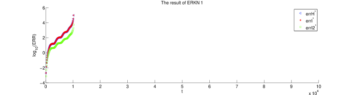
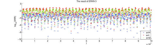
Figure 1: The errors against $t$ for ERKN 1 (up) and 3 (down).

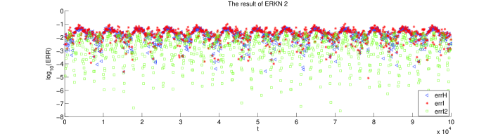
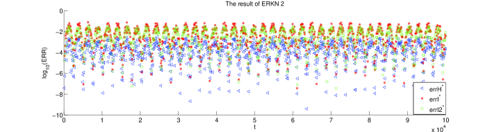
Figure 2: The errors of energies (up) and modified energies (down) against $t$ for ERKN 2.

From the numerical results, it follows that the non-symmetric ERKN1 can not preserve the energies and the symmetric and symplectic ERKN3 can approximately conserve the energies very well over long times. For the symmetric ERKN 2 and 4 not satisfying the condition (26), they approximately conserve the modified energies better than the original energies.

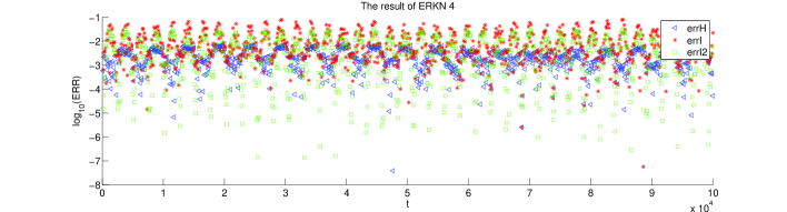
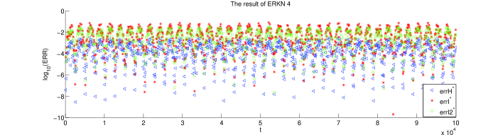
Figure 3: The errors of energies (up) and modified energies (down) against $t$ for ERKN 4.

7 Conclusions

This paper studied the long-time behaviour of ERKN integrators for muti-frequency highly oscillatory Hamiltonian systems. The modulated multi-frequency Fourier expansion of ERKN integrators were developed and by which, we showed the long-time numerical energy conservation of the integrators. Our next work will be devoted to the long-time analysis of ERKN integrators for multi-frequency highly oscillatory Hamiltonian systems under minimal non-resonance conditions.

References

• [1] Benettin, G., Galgani, L., Giorgilli, A.: Realization of holonomic constraints and freezing of high frequency degrees of freedom in the light of classical perturbation theory. II. Comm. Math. Phys. 121, 557–601 (1989)
• [2] Cohen, D.: Conservation properties of numerical integrators for highly oscillatory Hamiltonian systems. IMA J. Numer. Anal. 26, 34–59 (2006)
• [3] Cohen, D., Gauckler, L.: One-stage exponential integrators for nonlinear Schrödinger equations over long times. BIT 52, 877–903 (2012)
• [4] Cohen, D., Gauckler, L., Hairer, E., Lubich, C.: Long-term analysis of numerical integrators for oscillatory Hamiltonian systems under minimal non-resonance conditions. BIT 55, 705–732 (2015)
• [5] Cohen, D., Hairer, E., Lubich, C.: Modulated Fourier expansions of highly oscillatory differential equations. Found. Comput. Math. 3, 327–345 (2003)
• [6] Cohen, D., Hairer, E., Lubich, C.: Numerical energy conservation for multi-frequency oscillatory differential equations. BIT 45, 287–305 (2005)
• [7] Cohen, D., Jahnke, T., Lorenz, K., Lubich, C.: Numerical integrators for highly oscillatory Hamiltonian systems: a review. in Analysis, Modeling and Simulation of Multiscale Problems (A. Mielke, ed.), Springer, Berlin, 553–576 (2006)
• [8] Gauckler, L., Lubich, C.: Splitting integrators for nonlinear Schrödinger equations over long times. Found. Comput. Math. 10, 275–302 (2010)
• [9] Grimm, V., Hochbruck, M.: Error analysis of exponential integrators for oscillatory second-order differential equations. J. Phys. A: Math. Gen. 39, 5495–5507 (2006)
• [10] Hairer, E., Lubich, C.: Long-time energy conservation of numerical methods for oscillatory differential equations. SIAM J. Numer. Anal. 38, 414–441 (2000)
• [11] Hairer, E., Lubich, C.: Oscillations over long times in numerical Hamiltonian systems, in Highly oscillatory problems (B. Engquist, A. Fokas, E. Hairer, A. Iserles, eds.). London Mathematical Society Lecture Note Series 366, Cambridge Univ. Press (2009)
• [12] Hairer, E., Lubich, C.: Modulated Fourier expansions for continuous and discrete oscillatory systems. Foundations of Computational Mathematics: Budapest 2011 (F. Cucker et al., eds.), Cambridge Univ. Press, 113–128 (2012)
• [13] Hairer, E., Lubich, C.: Long-term analysis of the Störmer-Verlet method for Hamiltonian systems with a solution-dependent high frequency. Numer. Math. 134, 119–138 (2016)
• [14] Hairer, E., Lubich, C., Wanner G.: Geometric Numerical Integration: Structure-Preserving Algorithms for Ordinary Differential Equations. 2nd edn. Springer-Verlag, Berlin (2006)
• [15] Hochbruck, M., Lubich, C.: A Gautschi-type method for oscillatory second-order differential equations. Numer. Math. 83, 403–426 (1999)
• [16] Hochbruck, M., Ostermann, A.: Exponential integrators. Acta Numer. 19, 209–286 (2010)
• [17] Iserles, A., Nørsett, S.P.: From high oscillation to rapid approximation I: Modified Fourier expansions. IMA J. Numer. Anal. 28, 862–887 (2008)
• [18] Li, Y.W., Wu, X.: Exponential integrators preserving first integrals or Lyapunov functions for conservative or dissipative systems. SIAM J. Sci. Comput. 38, 1876–1895 (2016)
• [19] McLachlan, R.I., Stern, A.: Modified trigonometric integrators. SIAM J. Numer. Anal. 52, 1378–1397 (2014)
• [20] Sanz-Serna, J.M.: Modulated Fourier expansions and heterogeneous multiscale methods. IMA J. Numer. Anal. 29, 595–605 (2009)
• [21] Stern, A., Grinspun, E.: Implicit-explicit variational integration of highly oscillatory problems. Multi. Model. Simul. 7, 1779–1794 (2009)
• [22] Wang, B., Iserles, A., Wu, X.: Arbitrary-order trigonometric Fourier collocation methods for multi-frequency oscillatory systems. Found. Comput. Math. 16, 151–181 (2016)
• [23] Wang, B., Meng, F., Fang, Y.: Efficient implementation of RKN-type Fourier collocation methods for second-order differential equations. Appl. Numer. Math. 119, 164–178 (2017)
• [24] Wang, B., Wu, X.: Long-time numerical energy conservation of extended RKN integrators for highly oscillatory Hamiltonian systems. Preprint, arXiv:1712.04969 (2017)
• [25] Wang, B., Wu, X.: Functionally-fitted energy-preserving integrators for Poisson systems. J. Comput. Phys. 364, 137–152 (2018)
• [26] Wang, B., Wu, X., Meng, F.: Trigonometric collocation methods based on Lagrange basis polynomials for multi-frequency oscillatory second-order differential equations. J. Comput. Appl. Math. 313, 185–201 (2017)
• [27] Wang, B., Wu, X., Xia, J.: Error bounds for explicit ERKN integrators for systems of multi-frequency oscillatory second-order differential equations. Appl. Numer. Math. 74, 17–34 (2013)
• [28] Wu, X., Wang, B.: Explicit symplectic multidimensional exponential fitting modified Runge–Kutta–Nystrom methods. BIT 52, 773–795 (2012)
• [29] Wu, X., You, X., Shi, W., Wang, B.: ERKN integrators for systems of oscillatory second-order differential equations. Comput. Phys. Comm. 181, 1873–1887 (2010)
• [30] Wu, X., You, X., Wang, B.: Structure-preserving algorithms for oscillatory differential equations. Springer-Verlag, Berlin (2013)