Abstract

In this report, we introduce the concept of Rician $K$-factor-based radio resource and mobility management for fifth generation (5G) ultra-dense networks (UDN), where the information on the gradual visibility between the new radio node B (gNB) and the user equipment (UE)—dubbed X-line-of-sight (XLOS)—would be required. We therefore start by presenting the XLOS service probability as a new performance indicator; taking into account both the UE serving and neighbor cells. By relying on a lognormal $K$-factor model, a closed-form expression of the XLOS service probability in a 5G outdoor UDN is derived in terms of the multivariate Fox H-function; wherefore we develop a GPU-enabled MATLAB routine and automate the definition of the underlying Mellin-Barnes contour via linear optimization. Residue theory is then applied to infer the relevant asymptotic behavior and show its practical implications. Finally, numerical results are provided for various network configurations, and underpinned by extensive Monte-Carlo simulations.

I Introduction

The emergence of massive-MIMO and millimeter-wave (mmWave) as key enablers for 5G ultra-dense networks [MIMO_mmWave] will certainly prompt the reshaping of radio resource and mobility management algorithms, wherefore a new set of measured quantities might be required as inputs. In this context, the Rician $K$-factor can serve as an accurate channel metric to measure the gradual visibility condition of a radio link, termed X-line-of-sight (XLOS) here, and encompassing LOS, obstructed-LOS (OLOS) and non-LOS (NLOS) as discrete regimes. In localization services for instance, while the availability of a LOS path is quintessential for the classical triangulation-based schemes such as time-of-arrival (TOA) and direction-of-arrival (DOA), the massive-MIMO-based space-time processing approaches can deliver very concise localization thanks to the high angular resolution of the large scale antennas, and may therefore operate in the worst OLOS/NLOS conditions, yet at the expense of a higher complexity [Localization]. To optimize the computational cost, an operator may adopt a hybrid network configuration where, according to a fine-tuned target $K$-factor threshold, the 5G gNB can switch between the simpler conventional methods and the massive-MIMO ones. On the other hand, in future UDNs with co-located sub-6GHz/mmWave deployment, operators might configure only an anchor internet of things (IoT) carrier on the sub-6GHz—given the scarcity of spectrum—and offload a great part of the traffic to mmWave stand-alone IoT carriers. For energy savings considerations, the 5G network might prevent IoT devices from performing the periodic inter-frequency measurements and reporting by triggering blind inter-frequency re-selections [NB-IoT] to a mmWave IoT carrier once the sub-6GHz $K$-factor exceeds a preset threshold. Zooming out from the applications, a mathematical characterization of XLOS is yet to be established.

In this letter, we propose the XLOS service probability as a performance indicator, and start by introducing a broader definition of the concept thereof; accommodating the monitoring of both the UE serving and neighbor cells. By invoking a distance-based lognormal $K$-factor model for outdoor fixed and/or sporadically moving UEs [Greenstein], we then derive—in terms of the multivariate Fox H-function [Mathai2, A.1]—a closed-form expression for the XLOS service probability in a 5G OFDMA-based multi-tier heterogeneous network (HetNet), where a majority of cellular IoT devices and outdoor customer premise equipments (CPEs) are either fixed or changing their locations in an intermittent manner (e.g., position sensors with event-driven reporting) [NB-IoT], and where the $K$-factor variations stem also from the movement of the scattering objects (e.g., vehicles, containers, windblown leaves). Finally, the asymptotic behavior highlighting the effect of different network and channel parameters is studied using the residue theory.

II System Model

Consider an outdoor 2 GHz orthogonal frequency division multiple access (OFDMA)-based 5G [NR_OFDM] $N$-tiers UDN, where each cell class $n$ $(n=1,\ldots,N)$ is modeled as a homogeneous Poisson point process (PPP) $\Phi_{n}$, and distinguished by its deployment density $\lambda_{n}$, maximum transmit power per resource element (RE) $P_{n}$, antennas height $h_{n}$ and beamwidth $\theta_{n}$. The corresponding channel is presenting a large scale fading, with constant path-loss exponent $\nu$ and lognormal shadowing $\mathcal{X}_{n}$ of mean $\mu_{n}$ and standard deviation $\sigma_{n}$. Assuming that UE locations follow an independent PPP $\Phi_{u}$ of density $\lambda_{u}$, the downlink analysis is performed at a typical UE located at the origin [Stochastic_Geometry_book]. To model a massive IoT and CPE device ecosystem, we further suppose that UE locations are initially fixed, but may change every now and then.

II-A Cell Monitoring Criteria

As we are dealing with an outdoor context, we suppose that all tier’s cells are open access (including femtocells). We also adopt a reference signal receive power (RSRP)-based cell selection, wherein each UE periodically monitors the collection of the $M$ strongest cells, dubbed here monitoring set, and ends up connecting to the best server. Since UE measurements rely on the long-term frequency-domain post-equalization receive power, small-scale fading variations do not impact cell selection/reselection and are not, therefore, reflected in the actual RSRP that reads

$$P_{x_{n}}=P_{n}\mathcal{X}_{n}{\|x_{n}\|}^{-\nu},$$ (1)

where ${\|x_{n}\|}^{-\nu}$ stands for the standard path-loss between a typical UE and an $n^{\text{th}}$-tier BS located at ${x_{n}}\in\Phi_{n}$.

II-B $K$-Factor Model

The $K$-factor–like all large scale parameters (LSPs)–follows a lognormal distribution with mean and variance depending on the frequency band, environment and transmission/reception schemes (cf. [TR38901], [MeanVar] and references therein). Without loss of generality, let us adopt the findings of [Greenstein] for instance, where we assume that the narrowband $K$-factor periodically measured by a UE at independent positions can be empirically modeled for the $n\textsuperscript{th}$-tier as,

$$K_{x_{n}}=K_{n}\gamma_{n}{\|x_{n}\|}^{-\alpha},$$ (2)

where $\alpha>0$, $K_{n}$ is the $K$-factor intercept defined as

$$K_{n}=\left(h_{n}/h_{0}\right)^{\kappa_{1}}\left(\theta_{n}/\theta_{0}\right)^{\kappa_{2}}K_{0},$$ (3)

with $\kappa_{1}>0$, $\kappa_{2}<0$, $K_{0}>0$, and $\gamma_{n}$ is an independent lognormal variable, whose decibel value is zero mean with a standard deviation $\sigma_{K}$. Accurate values of these model parameters can be obtained through a calibration process according to the target environment. New Jersey’s measurement campaign in [Greenstein], for instance, yields $h_{0}=3\,\mathrm{m}$, $\theta_{0}=17\degree$, $\alpha=0.5$, $\kappa_{1}=0.46$, $\kappa_{2}=-0.62$, $K_{0}=10$, and $\sigma_{K}=8\,\mathrm{dB}$.

II-C Equivalent Formulation

Since manipulating distances in PPPs is easier, let us transform the RSRP process (1) into a simple unit-power PPP $\widetilde{\Phi}_{n}$, where the strongest power would correspond to the nearest neighbor cell to the typical UE. By invoking the random displacement theorem [Stochastic_Geometry_book, 1.3.9], [Shotgun, Corollary 3] shows that the two-dimensional (2D) process (1) is equivalent to another 2D process $P_{y_{n}}={\|y_{n}\|}^{-\nu}$, such that $y_{n}\in\widetilde{\Phi}_{n}$ with density $\widetilde{\lambda}_{n}=\lambda_{n}\Omega_{n}$, where $\Omega_{n}=P_{n}^{2/\nu}\mathbf{E}\left[\mathcal{X}_{n}^{2/\nu}\right]$ and the finite lognormal fractional moment $\mathbf{E}\left[\mathcal{X}_{n}^{2/\nu}\right]=\exp\left[\frac{\mathrm{ln}10}{5}\frac{\mu_{n}}{\nu}+\frac{1}{2}\left(\frac{\mathrm{ln}10}{5}\frac{\sigma_{n}}{\nu}\right)^{2}\right]$. By means of the mapping theorem [Stochastic_Geometry_book, 1.3.11], the $K$-factor can also be re-expressed as

$$K_{y_{n}}=K_{n}\gamma_{n}\Omega_{n}^{-\alpha/2}{\|y_{n}\|}^{-\alpha},\,y_{n}\in\widetilde{\Phi}_{n}.$$ (4)

III XLOS Service Probability

XLOS service probability in the vicinity of a UE, $P_{\mathrm{XLOS}}$, is defined as the probability that at least one cell in the monitoring set presents a $K$-factor higher than a threshold, say $K_{\mathrm{th}}$, that can be fine-tuned depending on the target service, i.e.,

$$P_{\mathrm{XLOS}}\left(K_{\mathrm{th}}\right)\triangleq\mathbf{Pr}\left[\bigcup_{m=1}^{M}K_{y_{n_{m}}}>K_{\mathrm{th}},\mathbf{n}\in\mathcal{M}\right],$$ (5)

where $\mathbf{n}=\left(n_{1},\ldots,n_{M}\right)$ and $\mathcal{M}=\{1,\ldots,N\}^{M}$. In the sequel, we derive a closed-form expression for the XLOS service probability and study its asymptotic behavior.

III-A Closed-Form Analysis

Using the total probability theorem as well as the independence between $\gamma_{n_{m}},\,m=1,\ldots,M$, the definition (5) can be rewritten as

$$\begin{split}P_{\mathrm{XLOS}}\left(K_{\mathrm{th}}\right)&=1-\mathbf{Pr}\left[\bigcap_{m=1}^{M}K_{y_{n_{m}}}\leq K_{\mathrm{th}},\mathbf{n}\in\mathcal{M}\right]\\ &=1-\sum_{\mathbf{n}\in\mathcal{M}}\mathbf{Pr}\left[y_{n_{m}}\in\widetilde{\Phi}_{n_{m}},m=1,\ldots,M\right]\\ &\hskip 45.5244pt\times\bigintsss_{0}^{z_{n_{2}}}\ldots\bigintsss_{0}^{z_{n_{M}}}\bigintsss_{0}^{+\infty}\prod_{m=1}^{M}\mathrm{CDF}_{\gamma_{n_{m}}}\left(\frac{K_{\mathrm{th}}\Omega_{n_{m}}^{\alpha/2}z_{n_{m}}}{K_{n_{m}}}\Bigg{|}z_{n_{m}}\right)f\left(z_{n_{1}},\ldots,z_{n_{M}}\right)\mathrm{d}z_{n_{1}}\ldots\mathrm{d}z_{n_{M}},\end{split}$$ (6)

where $z_{n_{m}}={\|y_{n_{m}}\|}^{\alpha}$ and $f\left(\cdot\right)$ is the joint probability density function (PDF) whose variables verify $0\leq z_{n_{1}}\leq z_{n_{2}}\leq\ldots\leq z_{n_{M}}$. Moreover, the independence between the homogeneous PPPs $\widetilde{\Phi}_{n_{m}}$ as well as the superposition theorem [Stochastic_Geometry_book, 1.3.3] imply that the sampling probability $\mathbf{Pr}\left[y_{n_{m}}\in\widetilde{\Phi}_{n_{m}},m=1,\ldots,M\right]=\prod_{m=1}^{M}\rho_{n_{m}}$, where $\rho_{n_{m}}=\widetilde{\lambda}_{n_{m}}/\lambda_{T}$ and $\lambda_{T}=\sum_{n=1}^{N}\widetilde{\lambda}_{n}$. To further develop (6), let us introduce the following new theorem.

Theorem 1 (Unified Expression for the Product of Lognormal CDFs).

Consider $M$ independent lognormal random variables $\gamma_{m}\,\left(m=1,\ldots,M\right)$, with mean $\mu_{m}(\mathrm{dB})$ and standard deviation $\sigma_{m}(\mathrm{dB})$. A unified expression for the product of their individual CDFs—that is equal to their joint CDF $\mathrm{CDF}_{\gamma_{1},\ldots,\gamma_{M}}\left(\gamma_{\mathrm{th},1},\ldots,\gamma_{\mathrm{th},M}\right)$—is given by

$$\prod_{m=1}^{M}\mathrm{CDF}_{\gamma_{m}}\left(\gamma_{\mathrm{th},m}\right)=\frac{1}{\pi^{M/2}}\sum_{l=1}^{L}w_{l}\prod_{m=1}^{M}\mathrm{H}_{1,1}^{0,1}\left[\frac{\gamma_{\mathrm{th},m}}{\omega_{l,m}}\begin{array}[]{|c}(1,1)\\ (0,1)\end{array}\right],$$ (7)

where $\omega_{l,m}=10^{(\sqrt{2}\sigma_{m}u_{l,m}+\mu_{m})/10}$ for $l\in\{1,\ldots,L\}$, $w_{l}$ and $\left(u_{l,1},\ldots,u_{l,M}\right)$ are respectively the weight and the $M$ abscissas of the $L^{\mathit{th}}$-order $M$-dimensional Gaussian weight Stroud monomial cubature [Stroud, Cools], with $\sum_{l=1}^{L}w_{l}=\pi^{M/2}$.

Proof.

cf. Appendix A. ∎

On the other hand, an explicit expression of the joint PDF $f(\cdot)$ can be obtained via the following corollary.

Corollary 1 (of Theorem [Distance, Appendix]).

In a multi-tier random network modeled in terms of $N$ independent PPPs $\widetilde{\Phi}_{n}\left(n=1,\ldots,N\right)$ with densities $\widetilde{\lambda}_{n}$, let $z_{m}=r_{m}^{\alpha}\left(m=1,\ldots,M\right)$, such that $r_{m}$ is the distance of the $m^{th}$ neighbor with respect to a certain origin. The joint PDF of $z_{1},\ldots,z_{M}$ unconditionally to $\{\widetilde{\Phi}_{n}\}$ reads

$$f\left(z_{1},\ldots,z_{M}\right)=\left(\frac{2\pi\lambda_{T}}{\alpha}\right)^{M}e^{-\pi\lambda_{T}z_{M}^{2/\alpha}}\prod_{m=1}^{M}z_{m}^{2/\alpha-1},\vspace{-3mm}$$ (8)

where $\lambda_{T}=\sum_{n=1}^{N}\widetilde{\lambda}_{n}$.

Proof.

cf. Appendix B. ∎

By making use of the aforementioned sampling probability as well as Theorem 1 and Corollary 1, the XLOS service probability (6) can be rewritten after some algebraic manipulations as,

$$\begin{split}P_{\mathrm{XLOS}}\left(K_{\mathrm{th}}\right)&=1-\left(\frac{2\sqrt{\pi}}{\alpha}\right)^{M}\sum_{\mathbf{n}\in\mathcal{M}}\prod_{m=1}^{M}\widetilde{\lambda}_{n_{m}}\sum_{l=1}^{L}w_{l}\times I_{1},\end{split}$$ (9)

where the multidimensional integral $I_{1}$ is expressed as

$$\begin{split}I_{1}&=\bigintsss_{0}^{z_{n_{2}}}\ldots\bigintsss_{0}^{z_{n_{M}}}\bigintsss_{0}^{+\infty}\prod_{m=1}^{M}z_{n_{m}}^{2/\alpha-1}\mathrm{H}_{1,1}^{0,1}\left[\frac{K_{\mathrm{th}}\Omega_{n_{m}}^{\alpha/2}z_{n_{m}}}{\omega_{l,m}K_{n_{m}}}\begin{array}[]{|c}(1,1)\\ (0,1)\end{array}\right]\times e^{-\pi\lambda_{T}z_{n_{M}}^{2/\alpha}}\,\mathrm{d}z_{n_{1}}\ldots\mathrm{d}z_{n_{M}}.\end{split}\vspace{-1.5mm}$$ (10)

$$\footnotesize I_{1}=\frac{\alpha}{2}\left(\pi\lambda_{T}\right)^{-M}\mathrm{H}_{M,M-1\colon\mathop{\mathchoice{\underbrace{\displaystyle 1,1\colon\ldots\colon 1,1}}{\underbrace{\textstyle 1,1\colon\ldots\colon 1,1}}{\underbrace{\scriptstyle 1,1\colon\ldots\colon 1,1}}{\underbrace{\scriptscriptstyle 1,1\colon\ldots\colon 1,1}}}\limits_{M\mathrm{-times}}}^{\hskip 4.55244pt0,M\hskip 9.6739pt\colon\hskip 1.42262pt0,1\colon\ldots\colon 0,1}\left[\begin{matrix}\frac{K_{\mathrm{th}}\Lambda_{n_{1}}^{\alpha/2}}{\omega_{l,1}K_{n_{1}}}\\ \vdots\\ \frac{K_{\mathrm{th}}\Lambda_{n_{M}}^{\alpha/2}}{\omega_{l,M}K_{n_{M}}}\end{matrix}\,\,\middle|\,\begin{matrix}\left(1-\frac{2i}{\alpha};\mathds{1}_{1\leq i},\ldots,\mathds{1}_{M\leq i}\right)_{1\leq i\leq M-1},\left(1-M;\mathop{\mathchoice{\overbrace{\displaystyle\frac{\alpha}{2},\ldots,\frac{\alpha}{2}}}{\overbrace{\textstyle\frac{\alpha}{2},\ldots,\frac{\alpha}{2}}}{\overbrace{\scriptstyle\frac{\alpha}{2},\ldots,\frac{\alpha}{2}}}{\overbrace{\scriptscriptstyle\frac{\alpha}{2},\ldots,\frac{\alpha}{2}}}}\limits^{M-\mathrm{times}}\right)\\ \left(-\frac{2i}{\alpha};\mathds{1}_{1\leq i},\ldots,\mathds{1}_{M\leq i}\right)_{1\leq i\leq M-1}\end{matrix}\,\middle|\,\begin{matrix}\left(1,1\right)\\ \left(0,1\right)\end{matrix}\,\middle|\,\begin{matrix}\ldots\end{matrix}\,\middle|\,\begin{matrix}\left(1,1\right)\\ \left(0,1\right)\end{matrix}\right]\vspace{-3.25mm}\normalsize$$ (15)

To derive a closed-form solution for (10), let us recall the representation of the involved Fox H-functions in terms of Mellin-Barnes integrals [Mathai2, Eq. (1.1.1)], i.e,

$$\mathrm{H}_{1,1}^{0,1}\left[z\,\begin{array}[]{|c}(1,1)\\ (0,1)\end{array}\right]=\frac{1}{2\pi j}\bigintsss_{\mathcal{C}_{m}}\phi\left(\zeta_{m}\right)z^{\zeta_{m}}\,\mathrm{d}\zeta_{m},$$ (11)

where $\phi\left(\zeta_{m}\right)=\Gamma\left(\zeta_{m}\right)/\Gamma\left(1+\zeta_{m}\right)$, and contours $\mathcal{C}_{m}\,\left(m=1,\ldots,M\right)$ are defined such that $\real\left(\zeta_{m}\right)>0$; the highest pole on the left. Combining (11) with (10) and interchanging the order of the real and contour integrals yields

$$\begin{split}I_{1}&=\left(\frac{1}{2\pi j}\right)^{M}\bigintsss_{\mathcal{C}_{1}}\ldots\bigintsss_{\mathcal{C}_{M}}\Psi\left(\zeta_{1},\ldots,\zeta_{M}\right)\times\prod_{m=1}^{M}\phi\left(\zeta_{m}\right)\left(\frac{K_{\mathrm{th}}\Omega_{n_{m}}^{\alpha/2}}{\omega_{l,m}K_{n_{m}}}\right)^{\zeta_{m}}\,\mathrm{d}\zeta_{1}\ldots\mathrm{d}\zeta_{M},\end{split}$$ (12)

with the multivariate term $\Psi$ given by

$$\begin{split}\Psi\left(\zeta_{1},\ldots,\zeta_{M}\right)&=\bigintsss_{0}^{z_{n_{2}}}\ldots\bigintsss_{0}^{z_{n_{M}}}\bigintsss_{0}^{+\infty}e^{-\pi\lambda_{T}z_{n_{M}}^{2/\alpha}}\times\prod_{m=1}^{M}z_{n_{m}}^{2/\alpha+\zeta_{m}-1}\,\mathrm{d}z_{n_{1}}\ldots\mathrm{d}z_{n_{M}}.\end{split}$$ (13)

Given that $\alpha\in\mathbb{R}^{+*}$ and $\real\left(\zeta_{m}\right)>0$, and using the identity $1/a=\Gamma\left(a\right)/\Gamma\left(1+a\right)$, the iterated integrals with respect to $z_{n_{1}},\ldots,z_{n_{M-1}}$ in (13) can be successively resolved by induction. The resulting integral relating to $z_{n_{M}}$ is then obtained using [Table_of_Integrals, Eq. (3.478.1)], which leads to

$$\begin{split}\Psi\left(\zeta_{1},\ldots,\zeta_{M}\right)&=\frac{\alpha}{2}\left(\pi\lambda_{T}\right)^{-\left(M+\frac{\alpha}{2}\sum_{m=1}^{M}\zeta_{m}\right)}\times\Gamma\left(M+\frac{\alpha}{2}\sum_{m=1}^{M}\zeta_{m}\right)\prod_{i=1}^{M-1}\frac{\Gamma\left(\frac{2i}{\alpha}+\sum_{m=1}^{M}\mathds{1}_{m\leq i}\zeta_{m}\right)}{\Gamma\left(1+\frac{2i}{\alpha}+\sum_{m=1}^{M}\mathds{1}_{m\leq i}\zeta_{m}\right)}.\end{split}$$ (14)

By plugging (14) into (12), we recognize that integral $I_{1}$ can be re-expressed in terms of the multivariate Fox H-function [Mathai2, A.1] as given by (15) on top of this page, where parameter $\Lambda_{n_{m}}\triangleq\Omega_{n_{m}}/\pi\lambda_{T}$ is encompassing network density, power and shadowing effects. Finally, a closed-form expression for $P_{\mathrm{XLOS}}$ is deduced by substituting (15) in (9).

III-B Asymptotic Behavior

As depicted in Table I, the two asymptotic regimes of the ratio $K_{\mathrm{th}}\Lambda_{n_{m}}^{\alpha/2}/\omega_{l,m}K_{n_{m}}$ reflect many practical scenarios, wherefore it is interesting to establish the corresponding XLOS service probability expressions; denoted $\overline{P}_{\mathrm{XLOS}}$ in the sequel. Let $\mathcal{H}$ stand for the multivariate Fox H-function in (15) where

$$\mathcal{H}=\left(\frac{1}{2\pi j}\right)^{M}\bigintsss_{\mathcal{C}_{1}}\ldots\bigintsss_{\mathcal{C}_{M}}F\left(\zeta_{1},\ldots,\zeta_{M}\right)\,\mathrm{d}\zeta_{1}\ldots\mathrm{d}\zeta_{M}.$$ (16)

In view of the series representations of the monovariate Fox H-function [Kilbas, Theorem 1.2] (while noticing the inverted definition of the H-function therein), an asymptotic expression of (15) is obtained as follows.

Low ratio regime: Since the integrand $F$ has no poles on the right of the $M$ individual contours in (16), [Kilbas, Eq. (1.2.23)] implies that $\mathcal{H}\simeq 0$, and thereby $\overline{P}_{\mathrm{XLOS}}=1$.

High ratio regime: By applying [Kilbas, Eq. (1.2.22)] to the $M$ individual contour integrals, an approximation of $\mathcal{H}$ is given in terms of the residues of $F$ as

$$\begin{split}\mathcal{H}&\simeq\mathbf{Res}\left[F,\left(0,\ldots,0\right)\right]+\mathbf{Res}\left[F,\left(-\frac{2}{\alpha},0,\ldots,0\right)\right]\\[-5.69054pt] &\simeq\lim_{\zeta_{M}\rightarrow 0}\ldots\lim_{\zeta_{1}\rightarrow 0}\prod_{m=1}^{M}\zeta_{m}F\left(\zeta_{1},\ldots,\zeta_{M}\right)+\lim_{\zeta_{M}\rightarrow 0}\ldots\lim_{\zeta_{2}\rightarrow 0}\lim_{\zeta_{1}\rightarrow-\frac{2}{\alpha}}\left(\zeta_{1}+\frac{2}{\alpha}\right)\prod_{m=2}^{M}\zeta_{m}F\left(\zeta_{1},\ldots,\zeta_{M}\right),\end{split}\vspace{-1.5mm}$$ (17)

which evaluates to

$$\mathcal{H}\simeq\left(\frac{\alpha}{2}\right)^{M-1}\left[1-\left(\frac{K_{\mathrm{th}}\Lambda_{n_{1}}^{\alpha/2}}{\omega_{l,1}K_{n_{1}}}\right)^{2/\alpha}\right].\vspace{-1.5mm}$$ (18)

Finally, combining (9), (15) and (18), as well as recalling that $\sum_{l=1}^{L}w_{l}=\pi^{M/2}$, we obtain after some algebraic manipulations

$$\overline{P}_{\mathrm{XLOS}}=\frac{1}{\pi^{M/2-1}}\sum_{\mathbf{n}\in\mathcal{M}}\frac{\lambda_{T}}{\Omega_{n_{1}}}\prod_{m=1}^{M}\rho_{n_{m}}\sum_{l=1}^{L}w_{l}\left(\frac{\omega_{l,1}K_{n_{1}}}{K_{\mathrm{th}}}\right)^{2/\alpha}.$$ (19)

Table I: XLOS service probability asymptotic expressions

Case	Practical Scenarios	$\overline{P}_{\mathrm{XLOS}}$
$\frac{K_{\mathrm{th}}\Lambda_{n_{m}}^{\alpha/2}}{\omega_{l,m}K_{n_{m}}}\rightarrow 0$	•    Poor LOS (i.e., low $K_{\mathrm{th}}$), •    Fair LOS quality in a UDN with high power and narrow-beam antennas (i.e., high $\lambda_{T}$ and $K_{n_{m}}$).	$1$
$\frac{K_{\mathrm{th}}\Lambda_{n_{m}}^{\alpha/2}}{\omega_{l,m}K_{n_{m}}}\rightarrow+\infty$	•    High quality LOS (i.e., high $K_{\mathrm{th}}$), •    Fair LOS quality in a low density HetNet with low power and large beamwidth antennas (i.e., low $\lambda_{T}$ and $K_{n_{m}}$).	Equation (19)

IV Numerical Results and Mathematical Software

To validate our theoretical findings, we conduct Monte-Carlo simulations for three practical scenarios as depicted in Table II, and we adopt New Jersey’s calibration presented in II-B with $\sigma_{K}=3\,\mathrm{dB}$. The analytical expressions are evaluated via a degree-$11$ Stroud cubature for which $L=(4M^{5}-20M^{4}+140M^{3}-130M^{2}+96M+15)/15$. To that end, we make use of Stenger’s tabulations [Stenger] to update the Matlab code in [StroudMatlab]. Moreover, using the quasi Monte-Carlo framework, we introduce in Appendix C an efficient GPU-oriented MATLAB routine to calculate the multivariate Fox H-function. By translating the Mellin-Barnes contour constraints into a linear optimization problem, we come up with a code automating the contour definition in Appendix D. A test example is finally provided in Appendix E. Note that we have already introduced a C/MEX version of the multivariate Fox H-function in our package [mfoxh]. An excerpt of the source and test examples are presented in Appendices F and G, respectively. Also, a Python implementation for the same generalized function can be found in [Python].

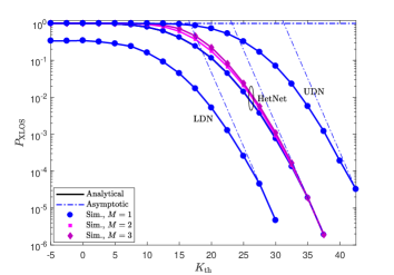
Figure 1: XLOS probability versus $K_{\mathrm{th}}$ for UDN, HetNet (Macro/Femto) and LDN. Path-loss exponent $\nu=3$ and shadowing mean $\mu_{n}=0$ for all tiers $n=1,\ldots,N$.

Fig. 1 shows that, in the UDN case, the low ratio asymptotic regime is easily established, and good LOS conditions (e.g., $K_{\mathrm{th}}=12\,\mathrm{dB}$) are obtained with probability 1. Conversely, the low density network (LDN) scenario unfolds in NLOS situations with non-negligible probability (e.g., $K<-5\,\mathrm{dB}$ with probability $0.5$). By considering the neighboring cells ($M=2,3$) in the HetNet (Macro/Femto) case for instance, we remark that a substantial increase of the XLOS probability is achieved only in the non-asymptotic regime. Indeed, a high $K_{\mathrm{th}}$ requirement can be fulfilled merely by the serving cell, since the $K$-factors of neighbor cells become limited by the corresponding path-losses.

Table II: Network and transmission settings

Case	$N$	$\lambda_{n}$	$P_{n}(\mathrm{dBm})$	$\theta_{n}(\degree)$	$h_{n}(\mathrm{m})$	$\sigma_{n}(\mathrm{dB})$
UDN	$1$	$3\times 10^{-2}$	$5.2$	$45$	$15$	5
HetNet	$2$	$10^{-5},5\times 10^{-4}$	$15.2,-4.8$	$39,180$	$25,10$	8, 4
LDN	$1$	$3\times 10^{-8}$	$5.2$	$65$	$30$	5

V Conclusion

In this letter, we have introduced the XLOS service probability as a new $K$-factor-based performance indicator, and provided its analytical and asymptotic expressions that establish a link between 5G network and transmission parameters and the gradual visibility condition of radio links. As exemplified in the introduction, by tweaking a $K$-factor threshold $K_{\mathrm{th}}$, the XLOS metric can be used by network optimization engineers as a switching probability between e.g., conventional localization schemes—requiring LOS—and Massive-MIMO ones operating in OLOS conditions. As a perspective, the adopted $K$-factor model from [Greenstein] can be extended to the vehicular case in future works.

Appendix A Proof of Theorem 1

First, by making a simple variable change, the product of lognormal PDFs $p_{\gamma_{m}},\ p=\prod_{m=1}^{M}p_{\gamma_{m}}$, can be reformulated as

$$\vspace{-1mm}p=\frac{1}{\pi^{M/2}}\bigintssss_{\mathbb{R}^{M}}e^{-\left(u_{1}^{2}+\ldots+u_{M}^{2}\right)}Q\left(u_{1},\ldots,u_{M}\right)\mathrm{d}u_{1}\ldots\mathrm{d}u_{M},\vspace{-1mm}$$ (20)

where $Q\left(u_{1},\ldots,u_{M}\right)=\prod_{m=1}^{M}\delta\left(\gamma_{m}-10^{(\sqrt{2}\sigma_{m}u_{m}+\mu_{m})/10}\right)$. By applying the Gaussian-weight Stroud monomial cubature [Stroud, Cools] to (20), and recalling that $\delta\left(\gamma_{m}-a\right)=\mathrm{H}_{0,0}^{0,0}\left[\frac{\gamma_{m}}{a}\begin{array}[]{|c}\rule{14.22636pt}{0.4pt}\\ \rule{14.22636pt}{0.4pt}\end{array}\right]$, we get

$$\vspace{-1mm}p=\frac{1}{\pi^{M/2}}\sum_{l=1}^{L}w_{l}\prod_{m=1}^{M}\mathrm{H}_{0,0}^{0,0}\left[\frac{\gamma_{m}}{\omega_{l,m}}\begin{array}[]{|c}\rule{14.22636pt}{0.4pt}\\ \rule{14.22636pt}{0.4pt}\end{array}\right],\vspace{-1mm}$$ (21)

with $w_{l}$ and $\left(u_{l,1},\ldots,u_{l,M}\right)$ are respectively the $l^{\mathrm{th}}$ weight and abscissas of the $M$-dimensional cubature, and $\omega_{l,m}=10^{(\sqrt{2}\sigma_{m}u_{l,m}+\mu_{m})/10}$. Finally, by invoking [Mathai2, Eq. (2.53)], the integration of (21) with respect to $\gamma_{m}$ from $0$ to $\gamma_{\mathrm{th,m}}\,(m=1,\ldots,M)$ leads to (7). $\blacksquare$

Appendix B Proof of Corollary 1

It immediately follows from applying the superposition theorem [Stochastic_Geometry_book, 1.3.3] to the equivalent PPP $\Phi_{T}=\bigcup_{n=1}^{N}\widetilde{\Phi}_{n}$, and performing a PDF transformation to the joint distance distribution of the first $M$ neighbors given by theorem [Distance, Appendix]. $\blacksquare$

Appendix C GPU-Enabled Multivariate Fox H-Function MATLAB Code

⬇

1function out = mfoxh(z, Contour, an, Alphan, ap, Alphap, bq, Betaq, varargin)

2% For dim >= 4, we recommend the use of GPU-enabled HPC servers

3% an = [a1,...,an] and Alphan = [alpha,1,1 ... alpha,n,1;...; alpha,1,r...alpha,n,r]

4% varargin form (i = 1 ..r): [ci,1 ...ci,n ; gammai,1 ... gammai,n],

5%[ci,n+1 ...ci,p ; gammai,n+1 ... gammai,p],

6%[di,1 ...di,m ; deltai,1 ... deltai,m], [di,m+1 ...di,q ; deltai,m+1 ... deltai,q]

7% See notation in A. Mathai, The H-function, Theory and Applications, Annex A.1

8%================================================================================================

9dim = size(Contour,1);

10

11N = 2^8 * 3^3 * 5^(2+dim); % For a better performance, N is made of powers of prime numbers

12%========================== Multivariate Quasi Monte-Carlo Integration ==========================

13p = haltonset(dim,’Skip’,1e3,’Leap’,1e2);

14p = scramble(p,’RR2’);

15in = gpuArray(net(p,N));

16G = gpuArray(ones(1,N));

17C = gpuArray(Contour);

18points = kron(G,C(:,1)) + kron(G, C(:,2)-C(:,1)).* in’;

19mceval = Integrand(points);

20mcsum = sum(mceval,2);

21v = prod(C(:,2) - C(:,1)); % volume

22out = v * mcsum / N; % Integral

23%========================================== Integrand ===========================================

24function f = Integrand(s)

25j = sqrt(-1);

26r = length(z);

27Nvar = length(varargin);

28for nvar = 1 : Nvar

29 if(isempty(cell2mat(varargin(nvar))))

30 varargin{nvar} = zeros(2,0);

31 end

32end

33Phi = 1;

34for i = 1 : r

35 cni = gpuArray(cell2mat(varargin(4*(i-1)+1)));

36 cpi = gpuArray(cell2mat(varargin(4*(i-1)+2)));

37 dmi = gpuArray(cell2mat(varargin(4*(i-1)+3)));

38 dqi = gpuArray(cell2mat(varargin(4*(i-1)+4)));

39 Phi = Phi .* ((GammaProd(1-cni(1,:),cni(2,:), s(i,:)).* GammaProd(dmi(1,:),-dmi(2,:), s(i,:)))...

40 ./(GammaProd(cpi(1,:),-cpi(2,:), s(i,:)).* GammaProd(1-dqi(1,:),dqi(2,:), s(i,:)))).* z(i).^s(i,:);

41end

42Psi = GammaProd(1-an,Alphan,s)./(GammaProd(ap,-Alphap,s).* GammaProd(1-bq,Betaq,s));

43f = (1/(2*j*pi)^r) * Phi .* Psi;

44end

45%========================================== GammaProd ===============================================

46function output = GammaProd(p,m,s)

47if (isempty(p)|| isempty(m))

48 output = ones(size(s(1,:)));

49else

50L1 = size(s,1);

51comb = 0;

52for i = 1 : L1

53[pp ss] = meshgrid(p,s(i,:));

54 mm = meshgrid(m(i,:),s(i,:));

55 comb = comb + mm .* ss;

56end

57 output = reshape(prod(gammas(pp + comb),2),size(s(1,:)));

58end

59end

60end

61% gammas function here is the complex gamma, available in

62% www.mathworks.com/matlabcentral/fileexchange/3572-gamma

63end

Appendix D Automatic Contour Generator

⬇

1function c = mfoxcontour(W, dim, an, Alphan, varargin)

2% an = [a1,...,an] and Alphan = [alpha,1,1 ... alpha,n,1;...; alpha,1,r...alpha,n,r]

3% varargin form (i = 1 ..r): [ci,1 ...ci,n ; gammai,1 ... gammai,n],

4% [di,1 ...di,m ; deltai,1 ... deltai,m]

5% See notation in A. Mathai, The H-function, Theory and Applications, Annex A.1

6% W : control the width of the integration interval in [-i\infty +i\infty]

7% dim : stands for the dimension

8

9Nvar = length(varargin);

10epsilon = 1/10;

11f = ones(1,dim);

12Q = -Alphan.’;

13b = 1-an-epsilon;

14lb = [];

15ub = [];

16

17for i = 1 : Nvar/2

18 cni = cell2mat(varargin(2*(i-1)+1)); % [c1,i ...cn,i;gamma_1,i...gamma_n,i]

19 if(isempty(cni)) cni = [-1e10;1]; end

20 dmi = cell2mat(varargin(2*(i-1)+2)); % [d1,i ...dm,i;delta_1,i...delta_m,i]

21 if(isempty(dmi)) dmi = [1e10;1]; end

22 lb = [lb max((cni(1,:)-1)./cni(2,:))]+epsilon;

23 ub = [ub min(dmi(1,:)./dmi(2,:))]-epsilon;

24end

25

26options = optimoptions(’linprog’,’Algorithm’,’interior-point’);

27out = linprog(f, Q, b, [], [], lb, ub, options);

28c = [out.’ - 1i * W; out.’ + 1i * W];

Appendix E MATLAB-GPU Test Code

In this example, we evaluate both a trivariate and bivariate Fox H-functions, respectively given by,

$$\mathrm{H}_{1}=\mathrm{H}_{2,1:1,0:1,0:1,0}^{0,1:0,1:0,1:0,1}\left(\begin{array}[]{c}3,2,0.5\end{array}\begin{array}[]{|c}\left(1.5;1,1,1\right),\left(2;1,1,1\right)\\ \left(2;1,1,1\right)\end{array}\begin{array}[]{|c}\_\\ \left(0,1\right)\end{array}\begin{array}[]{|c}\_\\ \left(3,1\right)\end{array}\begin{array}[]{|c}\_\\ \left(1,1\right)\end{array}\right),$$ (22)

and

$$\mathrm{H}_{2}=\mathrm{H}_{2,1:1,0:1,0}^{0,1:0,1:0,1}\left(\begin{array}[]{c}3,2\end{array}\begin{array}[]{|c}\left(1.5;1,1\right),\left(2;1,1\right)\\ \left(2;1,1\right)\end{array}\begin{array}[]{|c}\_\\ \left(0,1\right)\end{array}\begin{array}[]{|c}\_\\ \left(3,1\right)\end{array}\right).$$ (23)

The user may set the contour manually or generate it via mfoxcontour routine provided in Appendix D.

⬇

1% Trivariate example

2z = [3 2 0.5];

3an = [1.5];

4ap = [2];

5Alphan = [1 ; 1 ; 1];

6Alphap = [1 ; 1 ; 1];

7bq = [2];

8Betaq = [1 ; 1 ; 1];

9Contour = mfoxcontour(10, 3, an, Alphan, [],[0;1],[],[3;1],[],[1;1]);

10Contour =

11 -3.1000 -10.0000i -3.1000 +10.0000i

12 2.8000 -10.0000i 2.8000 +10.0000i

13 0.9000 -10.0000i 0.9000 +10.0000i

14H1 = mfoxh(z, Contour, an, Alphan, ap, Alphap, bq, Betaq,[],[],[0;1],[],[],[],[3;1],[],[],[],[1;1],[])

15H1 =

16 0.4886 + 0.0035i

17

18% Bivariate example

19z = [3 2];

20an = [1.5];

21ap = [2];

22Alphan = [1 ; 1];

23Alphap = [1 ; 1];

24bq = [2];

25Betaq = [1 ; 1];

26Contour = [-1.5-10i -1.5+10i ; 2.5-10i 2.5+10i]; % contour set manually

27H2 = mfoxh(z, Contour, an, Alphan, ap, Alphap, bq, Betaq,[],[],[0;1],[],[],[],[3;1],[])

28H2 =

29 -0.6014 + 0.0011i

Appendix F Parallel-CPU C/MEX Code: Excerpt from our Package [mfoxh]

⬇

1

2#include <omp.h>

3#include <stdio.h>

4#include <math.h>

5#include <gsl/gsl_qrng.h>

6#include <gsl/gsl_complex.h>

7#include <gsl/gsl_complex_math.h>

8#include <gsl/gsl_sf_gamma.h>

9#include <gsl/gsl_blas.h>

10#include <gsl/gsl_vector_complex_double.h>

11#include <gsl/gsl_matrix_complex_double.h>

12#include <gsl/gsl_matrix_int.h>

13#include "mfox.h"

14#include "mex.h"

15

16void mexFunction(int nlhs, mxArray *plhs[],

17 int nrhs, const mxArray *prhs[]){

18

19 size_t i, j, k, mx, nx, dim;

20 double *ind, *xr, *xi, *zr, *zi, *max_call, *tol;

21 gsl_complex x;

22 gsl_vector_complex *xl, *xu;

23 gsl_matrix_int *index;

24 gsl_matrix_complex *Arg[20], *Emp;

25

26if((nrhs -7) % 2 == 0){

27dim = (size_t)((nrhs -7)/2);}

28else{mexErrMsgTxt("Number of inputs is incorrect\n");}

29

30// Retrieve vector [0, n, m1, n1, …, mM, nM]

31if(mxIsComplex(prhs[0])){mexErrMsgTxt("Indices should be integers\n");}

32nx = mxGetN(prhs[0]);

33if(nx != 2*dim+2){mexErrMsgTxt("Missing input(s) or extra elements in the first argument (index)\n");}

34index = gsl_matrix_int_alloc(1, nx);

35ind = mxGetPr(prhs[0]);

36for(j = 0; j < nx; j++){

37gsl_matrix_int_set(index, 0, (const size_t)j, (int)ind[j]);

38}

39// Retrieve matrices Ai and Bi

40

41for(k = 0; k < nrhs-4; k++){

42if(! mxIsEmpty(prhs[k+1]))

43{

44 /* Get the length of each input vector. */

45 mx = mxGetM(prhs[k+1]);

46 nx = mxGetN(prhs[k+1]);

47 /* Check input parameters size */

48

49if(k == 0 && nx != dim){mexErrMsgTxt("Missing Fox H argument(s) z\n");}

50if(k > 0 && nx ==1){

51 mexPrintf("Error in parameter # %d\n",k+2);

52 mexErrMsgTxt("Input size is incorrect\n");

53 return;

54 }

55if(mxIsComplex(prhs[k+1])){

56 /* Get pointers to real and imaginary parts of the inputs. */

57 xr = mxGetPr(prhs[k+1]);

58 xi = mxGetPi(prhs[k+1]);

59

60 Arg[k] = gsl_matrix_complex_alloc(mx, nx);

61

62for(i = 0; i < mx; i++)

63 {

64 for(j = 0; j < nx; j++)

65 {

66 GSL_SET_COMPLEX(x,xr[i + mx*j],xi[i + mx*j]);

67 gsl_matrix_complex_set(Arg[k],

68 (const size_t)i, (const size_t)j, x);

69 }

70 }

71}//end of if

72

73else{

74/* Get pointers to real part */

75 xr = mxGetPr(prhs[k+1]);

76 Arg[k] = gsl_matrix_complex_alloc(mx, nx);

77

78for(i = 0; i < mx; i++)

79 {

80 for(j = 0; j < nx; j++)

81 {

82 GSL_SET_COMPLEX(x,xr[i + mx*j],0.0);

83 gsl_matrix_complex_set(Arg[k],

84 (const size_t)i, (const size_t)j, x);

85 }

86 }

87}//end of else

88}

89else{

90 Arg[k] = gsl_matrix_complex_alloc(2,1);

91 gsl_matrix_complex_set_all(Arg[k],GSL_COMPLEX_ONE);

92}

93}// end of for(k=0…

94// Retrieve integration intervals

95 if(mxGetN(prhs[nrhs-3]) < dim || mxGetM(prhs[nrhs-3]) < 2){

96 mexErrMsgTxt("Contour matrix size incorrect");

97 }

98 xl = gsl_vector_complex_alloc(dim);

99 xu = gsl_vector_complex_alloc(dim);

100/* Get pointers to real and imaginary parts of the inputs. */

101 xr = mxGetPr(prhs[nrhs-3]);

102 xi = mxGetPi(prhs[nrhs-3]);

103//Initialize integration domains

104for (i = 0; i < dim; i++) {

105 gsl_vector_complex_set (xl, i, gsl_complex_rect(xr[2*i],xi[2*i]));

106 gsl_vector_complex_set (xu, i, gsl_complex_rect(xr[2*i+1],xi[2*i+1]));

107}

108// Retrive max_call and tolerence

109if(!mxIsComplex(prhs[nrhs-2]) && !mxIsComplex(prhs[nrhs-1])){

110 max_call = mxGetPr(prhs[nrhs-2]);

111 tol = mxGetPr(prhs[nrhs-1]);

112 }

113else{mexErrMsgTxt("MaxFunEval and AbsTol must be real");}

114

115//Perform integration

116 gsl_complex result = GSL_COMPLEX_ZERO, error= GSL_COMPLEX_ZERO;

117 gsl_qrng* qrng = gsl_qrng_alloc(gsl_qrng_reversehalton, dim);

118/*Available sequences: gsl_qrng_halton, gsl_qrng_sobol, gsl_qrng_niederreiter_2, gsl_qrng_reversehalton*/

119 quasi_monte_state* s = quasi_monte_alloc(dim);

120 quasi_monte_integrate(xl, xu, dim, max_call[0], 0, tol[0], qrng, s, &result, &error, index, Arg);

121 quasi_monte_free(s);

122 gsl_qrng_free(qrng);

123/* Create a new complex array and set the output pointer to it. */

124 plhs[0] = mxCreateDoubleMatrix(1, 1, mxCOMPLEX);

125 zr = mxGetPr(plhs[0]);

126 zi = mxGetPi(plhs[0]);

127 zr[0] = GSL_REAL(result);

128 zi[0] = GSL_IMAG(result);

129}

Appendix G MEX Test Code: Excerpt from our Package [mfoxh]

⬇

1%***************************************** 2-Dimensions ****************************************

2 index = [0 1 1 1 1 1]; % [0 m m1 n1 m2 n2 ...mM nM]

3 z = [1 2]; % [z1...zM]

4 A = [1.5 1.0 1.0; 2.0 1.0 1.0]; % [a1 alpha_1,1...alpha_1,M; ...; ap alpha_p,1...alpha_p,M]

5 B = [2.0 1.0 1.0]; % [b1 beta_1,1...beta_1,M;...; bq beta_q,1 ...beta_q,M]

6 A1 = [-1 1]; % [a1_1 alpha1_1;...;a1_p1 alpha1_p1]

7 B1 = [0 1]; % [b1_1 beta1_1;...;b1_q1 beta1_q1]

8 A2 = [-1 1];

9 B2 = [3 1];

10 %c = [-0.5-10i 1.5-10i;-0.5+10i 1.5+10i];

11 c = mfoxcontour(10, 2, index, A, A1, B1, A2, B2);

12 % Tolerence settings

13 MaxFunEval = 2*1e5; % increase it to get more precision (especially for more than 2 dimensions)

14 AbsTol = 1e-4;

15 tic;

16 mfoxh(index, z, A, B, A1, B1, A2, B2, c, MaxFunEval, AbsTol)

17 toc;

18%***************************************** 3-Dimensions ****************************************

19 index = [0 1 1 1 1 1 1 1];

20 z = [1 2 0.5];

21 A = [1.5 1.0 1.0 1; 2.0 1.0 1.0 1];

22 B = [2.0 1.0 1.0 1];

23 A1 = [-1 1];

24 B1 = [0 1];

25 A2 = [-1 1];

26 B2 = [3 1];

27 A3 = [0 1];

28 B3 = [1 1];

29 %c = [-0.5-10i 1.5-10i 0.5-10i;-0.5+10i 1.5+10i 0.5+10i];

30 c = mfoxcontour(10, 3, index, A, A1, B1, A2, B2, A3, B3)

31 % Tolerence settings

32 MaxFunEval = 2*1e6; % increase it to get more precision (especially for more than 2 dimensions)

33 AbsTol = 1e-4;

34 tic;

35 mfoxh(index, z, A, B, A1, B1, A2, B2, A3, B3, c, MaxFunEval, AbsTol)

36 toc;

37%\end{lstlisting}

38\vspace{-2.5mm}

39\begin{thebibliography}{10}

40\vspace{-2.5mm}

41\bibitem[1]{Letter}H. Chergui, M. Benjillali and M.-S. Alouini, ‘‘Rician $K$-factor-based analysis of XLOS service probability in 5G outdoor ultra-dense networks,’’ Submitted as a Letter.

42\bibitem[2]{MIMO_mmWave}S. Sun \emph{et al.,} ‘‘MIMO for millimeter wave wireless communications: Beamforming, spatial multiplexing, or both?,’’ \emph{IEEE Comm. Mag.,} vol. 52, no. 12, pp. 110-121, Dec. 2014.

43\bibitem[3]{Localization}N. Garcia \emph{et al.,} ‘‘Direct localization for massive MIMO,’’ \emph{IEEE Trans. Sig. Proc.}, vol. 65, no. 10, pp 2475-2487, May 2017.

44\bibitem[4]{NB-IoT}3GPP, ‘‘Cellular system support for ultra-low complexity and low throughput Internet of Things (CIoT) (Release 13),’’ \textit{TR 45.820,} Nov. 2015.

45%\bibitem[4]{Cm_mmWave}M.-T. Martinez-Ingles \emph{et al.,} ‘‘Experimental comparison between centimeter and millimeter-wave ultrawideband radio channels,’’ in \emph{Radio Sci.}, vol. 49, no. 6, pp. 450-458, Jun. 2014.

46\bibitem[5]{Learning}F. B. Mismar and B. L. Evans, ‘‘Machine learning approach to estimating

47mmWave signal measurements during handover,’’ 2017. [Online]. Available: arxiv.org/abs/1710.01879.

48\bibitem[6]{Greenstein}L. J. Greenstein \emph{et al.,} ‘‘Ricean $K$-factors in narrow-band fixed wireless channels: Theory, experiments, and statistical models,’’\textit{IEEE Trans. Veh. Tech.,} vol. 58, no. 8, pp. 4000-4012, Oct. 2009.

49\bibitem[7]{Mathai2}A. M. Mathai, R. K. Saxena, and H. J. Haubold, \emph{The H-Function: Theory and Applications,} Springer, New York, 2010.

50\bibitem[8]{NR_OFDM}3GPP, ‘‘NR: Physical channels and modulation (Release 15),’’\textit{

51TS 38.211,} Sep. 2017.

52\bibitem[9]{Stochastic_Geometry_book} F. Baccelli and B. Blaszczyszyn, \textit{Stochastic Geometry and Wireless Networks, Volume I--Theory.} NOW: Foundations and Trends in

53Networking, 2009.

54\bibitem[10]{TR38901}3GPP, ‘‘Study on channel model for frequencies from 0.5 to 100 GHz (Release 14),’’ \textit{TR 38.901,} May. 2017.

55\bibitem[11]{MeanVar}H. Tataria \emph{et al.,} ‘‘Impact of Line-of-Sight and Unequal Spatial Correlation on Uplink MU-MIMO Systems,’’ \textit{IEEE Wireless Commun. Lett.,} vol. 6, no. 5, pp. 634-637, Oct. 2017.

56\bibitem[12]{Shotgun}P. Madhusudhanan \emph{et al.,} ‘‘Downlink performance analysis for a generalized shotgun cellular systems,’’ 2012. [Online]. Available: arxiv.org/abs/1002.3943.

57\bibitem[13]{Unified}F. Yilmaz and M.-S. Alouini, ‘‘A novel unified expression for the capacity and bit error probability of wireless communication systems over generalized fading channels,’’ \textit{IEEE Trans. Commun.,} vol. 60, no. 7, pp. 1862-1876, July 2012.

58\bibitem[14]{Stroud}A. H. Stroud, \emph{Approximate Calculation of Multiple Integrals}, Englewood Cliffs, N.J.:Prentice-Hall, 1971.

59\bibitem[15]{Cools}R. Cools and P. Rabinowitz, ‘‘Monomial cubature rules since ‘‘Stroud’’: a compilation,’’ \textit{Journal of Computational and Applied Mathematics,} vol. 48, no. 3, pp. 309-326, Nov. 1993.

60%\bibitem[17]{Mathai}A. Mathai and R. K. Saxena, \textit{The H-Function with Applications in Statistics and Other Disciplines,} John Wiley $\textrm{\&}$ Sons, Inc., 1978.

61\bibitem[16]{Table_of_Integrals}I. S. Gradshteyn and I. M. Ryzhik, \emph{Table of Integrals, Series, and Products}, 7th ed., Academic Press, 2007.

62\bibitem[17]{Kilbas}A. Kilbas and M. Saigo, \emph{H-Transforms: Theory and Applications. Analytical Methods and Special Functions}, Chapman \& Hall/CRC, Boca Raton-London-New York-Washington, D.C., 2004.

63\bibitem[18]{Stenger}F. Stenger, ‘‘Tabulation of certain fully symmetric numerical integration formulas of degree 7, 9 and 11,’’ \textit{Mathematics of Computation,} vol. 25, no. 116, pp. 935 and S58-S125, Oct. 1971.

64\bibitem[19]{StroudMatlab}J. Burkardt, ‘‘Stroud numerical integration in $M$ dimensions,’’ 2010. [Online]. Available: people.sc.fsu.edu/$\sim$jburkardt/m$\_$src/stroud/stroud.html.

65\bibitem[20]{mfoxh}H. Chergui, M. Benjillali and M.-S. Alouini, ‘‘Multivariate Fox H-Function C/MEX Package: mfoxh,’’ Zenodo, April, 2018. DOI: 10.5281/zenodo.1217925.

66\bibitem[21]{Python}H. R. Alhennawi \emph{et al.,} "Closed-form exact and asymptotic expressions for the symbol error rate and capacity of the $H$-function fading channel,’’ \textit{IEEE Trans. on Veh. Tech.}, vol. 65, no. 4, pp. 1957-1974, Apr. 2016.

67\bibitem[22]{Distance}H. R. Thompson, ‘‘Distribution of distance to nth neighbour in a population of

68randomly distributed individuals,’’ \emph{Ecology,} vol. 37, no. 2, pp. 391-394, Apr. 1956.

69\end{thebibliography}

70

71\end{document}