Many-particle mobility and diffusion tensors for objects in viscous sheets

Abstract

We derive a mobility tensor for many cylindrical objects embedded in a viscous sheet. This tensor guarantees a positive dissipation rate for any configuration of particles and forces, analogously to the Rotne-Prager-Yamakawa tensor for spherical particles in a three-dimensional viscous fluid. We test our result for a ring of radially driven particles, demonstrating the positive-definite property at all particle densities. The derived tensor can be utilized in Brownian Dynamics simulations with hydrodynamic interactions for such systems as proteins in biomembranes and inclusions in free-standing liquid films.

I Introduction

Many systems in nature are based on thin sheets of a viscous fluid. The main example is biomembranes SD . Other examples are soap films Weeks , liquid crystalline films Nguyen ; Qi and monolayers at fluid-fluid interfaces Prasad . Many studies have been devoted to the in-plain dynamics of such systems, some of which are reviewed in Ref. 6. These studies include, in particular, the derivation of the self-mobility of an isolated cylindrical particle in a viscous sheet Saffman ; Hughes , the pair-mobility of two such objects Naomi , as well as the hydrodynamic kernel associated with the flow due to a point-force LevineDyn ; LevineMob . We briefly review these results below. In addition, various numerical schemes were developed to deal with the complex membranal dynamics Brown ; Naji ; Camley ; Noruzifar .

The present work relates to the dynamics of multiple mobile objects within viscous sheets. As shown below, there are stability issues with the currently used many-particle mobility tensor, arising from the fact that it is not positive-definite. A similar problem is well-known in the case of particles in three-dimensional (3D) suspensions Zwanzig , and was famously solved by Rotne and Prager RP and Yamakawa Yamakawa . Here we solve it for the analogous quasi-two-dimensional (2D) case of viscous sheets.

We assume the usual limit of overdamped dynamics (vanishing Reynolds number). In this limit the response of the objects to forces is linear, instantaneous, and can be characterized by mobility coefficients. In biological systems these conditions generally apply SD ; Saffman . We focus on the translation of the objects and do not treat rotation. Along the text, we refer to mobilities ${\bf B}$ rather than diffusivities ${\bf D}$. At equilibrium, the two are related by the thermal energy, $ֿD=k_BTB$(theEinsteinrelation).\par Weproceedwithabriefsummaryofknownresultsforthemobilityofasingleparticleandapairofparticles,in3Dand2D.Thenwerefertomany-particledynamicsanddescribetheproblemofnegativemobilityanditscorrectionin3D.InSec.~{}\ref{sec_PDT}wederivea2Dmobilitytensor,whichispositive-definitebyconstruction.Weexaminethederivedtensorontwocases,testingitspositiveness.InSec.~{}\ref{sec_disc}wediscusstheresultsandpossibleextensionsandapplications.AppendicesA,B,andCprovideadditionalinformationwhichmaybeusefulforfuturesimulations.\par$

I.1 An isolated particle

The self-mobility of a particle, in general, characterizes its linear velocity response to the force applied to it,

$${\bf v}_{\alpha}={\bf B}_{{\rm s},\alpha\beta}{\bf F}_{\beta},$$ (1)

where Greek indices denote spatial coordinates, and we sum over repeated indices. In a 3D fluid of viscosity $\eta$, the self-mobility of a sphere of radius $a$ is given by Stokes’ formula StokesHappelBrenner ,

$${}^{{\rm 3D}}{\bf B}_{{\rm s},\alpha\beta}={}^{{\rm 3D}}B_{\rm s}\boldsymbol{\delta}_{\alpha\beta},\ \ \ ^{{\rm 3D}}B_{\rm s}=(6\pi\eta a)^{-1}.$$ (2)

In a viscous sheet of viscosity $\eta_{\rm s}$ and thickness $h$, the self-mobility of a particle of sufficiently small size $a$ is in general

$${}^{{\rm 2D}}{\bf B}_{{\rm s},\alpha\beta}={}^{{\rm 2D}}B_{\rm s}\boldsymbol{\delta}_{\alpha\beta},\ \ \ ^{{\rm 2D}}B_{\rm s}=\frac{1}{4\pi\mu}\left(\ln\frac{2}{\kappa a}-\gamma\right),\ \ \ \kappa a\ll 1.$$ (3)

Here $\mu=\eta_{\rm s}h$ is an effective 2D viscosity, $\gamma\simeq 0.58$ is Euler’s constant, and $\kappa^{-1}\gg a$ is an upper cut-off length required to regularize 2D hydrodynamics. In the specific example of the Saffman-Delbrück model for a protein in a biomembrane SD , illustrated in Fig. 1, the self-mobility is ${}^{{\rm 2D}}B_{\rm s}=(4\pi\mu)^{-1}[\ln(2\lambda/a)-\gamma]$. Here, the cut-off length $\kappa^{-1}$ is the Saffman-Delbrück length $\lambda=\mu/(2\eta)$, arising from the difference between the viscosities of the membrane and the surrounding fluid. Similar calculations for other viscous sheets and particle shapes all lead, in the limit $\kappa^{-1}\gg a$, to a self-mobility similar to Eq. (3), with varying definitions of the cut-off $\kappa$. Evans ; Stone ; NajiMob ; Daniels ; Henle ; Ramachandran

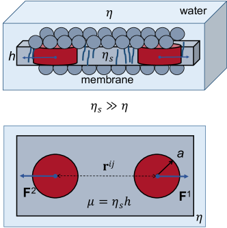
Figure 1: Illustration of a membrane of viscosity $\eta_{s}$ and thickness $h$, consisting of amphiphilic lipids (lighter, grey beads), with two driven proteins modeled as cylinders of radius $a$ (darker, maroon cylinders), immersed in a 3D surrounding fluid of viscosity $\eta$.

I.2 A pair of particles

When two or more particles move within a viscous fluid, they do not move independently. Mutual drag forces — hydrodynamic interactions — correlate their motions. For a single pair of particles Eq. (1) is generalized to

$${\bf v}^{i}_{\alpha}={\bf B}^{ij}_{\alpha\beta}\left({\bf r}\right){\bf F}^{j}_{\beta},$$ (4)

where the Latin indices $i,j=1,2$ mark the particles, and ${\bf r}={\bf r}^{2}-{\bf r}^{1}$ is the vector connecting their positions. Equation (4) describes the velocity response of each particle to the forces acting both on it and on its partner. The diagonal blocks ($i=j$) of the pair-mobility tensor give the self-mobility of each particle in the presence of its partner, given their separation ${\bf r}$, while the off-diagonal blocks ($i\neq j$) give their coupling due to the hydrodynamic interactions.

Within the Stokeslet approximation, valid in the limit of large separations compared to particle size ($r\gg a$), the particles are considered arbitrarily small, resulting in

$${\bf B}^{11}_{\alpha\beta}={\bf B}^{22}_{\alpha\beta}\simeq{\bf B}_{{\rm s},\alpha\beta},\ \ \ {\bf B}^{12}_{\alpha\beta}={\bf B}^{21}_{\alpha\beta}\simeq{\bf G}_{\alpha\beta}({\bf r}),$$ (5)

where ${\bf G}_{\alpha\beta}({\bf r})$ is the velocity response of the fluid at position ${\bf r}^{2}$ to a point-force at ${\bf r}^{1}$ (the Green’s function of the flow equations). Thus, in this limit, the diagonal block is just a self-mobility of an isolated particle, and the off-diagonal block is the coupling mobility of two point-like particles.

For a 3D suspension, the fluid’s response is given by the Oseen tensor Oseen ,

$${}^{{\rm 3D}}{\bf G}_{\alpha\beta}({\bf r})=\frac{1}{8\pi\eta r}\left(\boldsymbol{\delta}_{\alpha\beta}+\frac{{\bf r}_{\alpha}{\bf r}_{\beta}}{r^{2}}\right),$$ (6)

and the interaction strength decays with distance as $1/r$. This relatively slow decay corresponds to long-range hydrodynamic interactions between particles in suspensions.

For cylinders in a sheet, the analog of the Oseen tensor in the limit of $r\ll\kappa^{-1}$ is Lubensky ; Bussel ; LevineDyn ; LevineMob ; Naomi

$${}^{{\rm 2D}}{\bf G}_{\alpha\beta}({\bf r})=\frac{1}{4\pi\mu}\left[\left(\ln\frac{2}{\kappa r}-\gamma-\frac{1}{2}\right)\boldsymbol{\delta}_{\alpha\beta}+\frac{{\bf r}_{\alpha}{\bf r}_{\beta}}{r^{2}}\right].$$ (7)

Equations (3), (5), and (7) yield the pair-mobility tensor of two cylindrical particles within the Stokeslet approximation. The logarithmic decay with distance implies much longer-range correlations than in a 3D fluid, up to distances of order $\kappa^{-1}$. As a result, local perturbations give rise to strong nonlocal effects.

I.3 Many-particle dynamics

Let us consider an ensemble of many objects within a viscous sheet. In general, the velocity response of $N$ particles to the forces $\mathbb{F}=({\bf F}^{1},\ldots{\bf F}^{N})$ acting on them, is given by a many-particle mobility tensor, according to

$${\bf v}^{i}_{\alpha}={\bf B}^{ij}_{\alpha\beta}\left(\mathbbm{r}\right){\bf F}^{j}_{\beta},$$ (8)

where $i,j=1\ldots N$ are particle labels, and $\mathbbm{r}=({\bf r}^{1},...,{\bf r}^{N})$ is the configuration defined by the positions of all particles. A simple way to construct an approximate many-particle mobility tensor is to assume superposition of pair-mobilities. The pair-mobility in the Stokeslet approximation ($|{\bf r}^{ij}|\gg a$ for all pairs), Eq. (5), gives

$${\bf B}^{i=j}_{\alpha\beta}={\bf B}_{{\rm s},\alpha\beta},\ \ \ {\bf B}^{i\neq j}_{\alpha\beta}={\bf G}_{\alpha\beta}({\bf r}^{ij}),$$ (9)

where ${\bf r}^{ij}={\bf r}^{j}-{\bf r}^{i}$. Substitution of the expressions (2) and (6) for a 3D suspension in Eq. (9) yields the Kirkwood-Riseman (KR) tensor Kirkwood . The 2D-analog of this tensor is obtained by using the expressions (3) and (7) in Eq. (9) LevineMob .

I.4 Positive-definite mobility tensor

If the mobility tensor is not positive-definite, there exist configurations, for which the resulting power imparted to the particles,

$$\epsilon={\bf F}^{i}_{\alpha}{\bf v}^{i}_{\alpha}={\bf F}^{i}_{\alpha}{\bf B}^{ij}_{\alpha\beta}(\mathbbm{r}){\bf F}^{j}_{\beta},$$ (10)

is negative. However, in the viscous regime this power equals the energy dissipation rate in the fluid, which cannot be negative due to the second law of thermodynamics. The Stokeslet approximation fails to fulfill this requirement, as it becomes invalid once there are configurations with insufficiently large separations Zwanzig . The problem emerges, in particular, in Brownian Dynamics simulations, where configurations involving close-by particles are inevitable. The KR tensor gives rise to instability and non-physical dynamics in such simulations Zwanzig .

Rotne and Prager RP , and Yamakawa Yamakawa , calculated an improved tensor, which overcomes the problem of the KR tensor in 3D. The derivation by Rotne and Prager is based on an Ansatz for the stress tensor, taking into account the finite size of the particles, and integrating the flow response over their surfaces. This variational treatment yields a diffusion tensor, which goes beyond the Stokeslet limit. Although the tensor is not expected to be accurate for small separations, it (a) ensures a positive dissipation rate for all particle and force configurations, and (b) converges to the KR tensor for large separations. This Rotne-Prager-Yamakawa (RPY) tensor is given by

$${}^{{\rm 3D}}{\bf B}^{i=j}_{\alpha\beta}=^{{\rm 3D}}{\bf B}_{{\rm s},\alpha\beta},\ \ \ {}^{{\rm 3D}}{\bf B}^{i\neq j}_{\alpha\beta}=^{{\rm 3D}}{\bf G}_{\alpha\beta}({\bf r}^{ij})+{\bf C}({\bf r}^{ij}),$$ (11)

$${\bf C}({\bf r})=\frac{1}{12\pi\eta r}\frac{a^{2}}{r^{2}}\left(\boldsymbol{\delta}_{\alpha\beta}-3\frac{{\bf r}_{\alpha}{\bf r}_{\beta}}{r^{2}}\right),$$

where ${}^{{\rm 3D}}{\bf B}_{\rm s}$ remains the Stokes mobility of Eq. (2), and ${}^{{\rm 3D}}{\bf G}_{\alpha\beta}$ is the Oseen tensor, Eq. (6). Compared to the KR tensor of Eq. (9), the RPY tensor introduces a correction to second order in $a/r$. In fact, Eq. (11) is equivalent to a superposition of pair-mobilities, corrected to order $(a/r)^{2}$, which was not noted in the original paper.

Similarly, the negative mobility problem arises when using the 2D-analog of the KR tensor, obtained from Eqs. (3), (7), and (9). Here as well, the Stokeslet approximation fails for short-distance configurations, as will be demonstrated below. In the following section we apply the Rotne-Prager construction to the 2D case.

II 2D Positive-definite mobility tensor (PDT)

We follow the line of argument of Ref. 16 while adapting it to cylinders in a sheet. Since we restrict the discussion to distances $r\ll\kappa^{-1}$, the analysis is essentially two-dimensional, i.e., the dynamics is confined to the plane of the sheet. The effect of the 3D surroundings is captured by the cut-off $\kappa$ only. Thus, from now on we deal with a two-dimensional problem and omit the superscripts 2D.

Consider a configuration $\mathbbm{r}$ of cylindrical particles and forces $\mathbb{F}$ acting on them. The resulting exact flow field ${\bf u}({\bf r})$, satisfying the boundary conditions on the perimeters of all particles, is unknown. The stress tensor associated with it is $\boldsymbol{\sigma}_{\alpha\beta}({\bf r})=-p({\bf r})\boldsymbol{\delta}_{\alpha\beta}+\boldsymbol{\tau}_{\alpha\beta}({\bf r})$, where $p({\bf r})$ and $\boldsymbol{\tau}({\bf r})$ are the exact pressure and viscous-stress fields, with

$$\boldsymbol{\tau}_{\alpha\beta}({\bf r})=\mu\left[\partial_{\alpha}{\bf u}_{\beta}({\bf r})+\partial_{\beta}{\bf u}_{\alpha}({\bf r})\right].$$ (12)

Even though the exact stress tensor is unknown, it can be approximated, provided that the following basic properties are maintained. (a) Both $\boldsymbol{\sigma}$ and $\boldsymbol{\tau}$ are symmetric tensors, $\boldsymbol{\sigma}_{\alpha\beta}=\boldsymbol{\sigma}_{\beta\alpha}$ and $\boldsymbol{\tau}_{\alpha\beta}=\boldsymbol{\tau}_{\beta\alpha}$. (b) $\boldsymbol{\tau}$ is traceless, $\boldsymbol{\tau}_{\alpha\alpha}=0$. (c) The total stress tensor is divergenceless (local forces acting on a fluid element balance to zero since inertia is neglected),

$$\partial_{\beta}\boldsymbol{\sigma}_{\alpha\beta}({\bf r})=-\partial_{\alpha}p({\bf r})+\mu\partial_{\beta\beta}{\bf u}_{\alpha}({\bf r})=0.$$ (13)

(d) For the same reason, the total force exerted by the 2D flow on the perimeter of each particle exactly balances the external force applied to it,

$$a\int_{0}^{2\pi}d\theta\,\boldsymbol{\sigma}_{\alpha\beta}[{\bf r}^{i}+a{\bf n}^{i}(\theta)]\,{\bf n}^{i}_{\beta}(\theta)={\bf F}^{i}_{\alpha},$$ (14)

where ${\bf n}^{i}(\theta)$ is a unit normal to the perimeter of cylinder $i$. Once the viscous stress is formulated, one can obtain the mobility tensor by demanding that the total dissipation rate produced by the viscous flow must be equal to the power imparted to the particles by the external forces,

$$\epsilon=(2\mu)^{-1}\int d^{2}r\,\boldsymbol{\tau}_{\alpha\beta}\boldsymbol{\tau}_{\beta\alpha}={\bf F}^{i}_{\alpha}{\bf B}^{ij}_{\alpha\beta}(\mathbbm{r}){\bf F}^{j}_{\beta}.$$ (15)

Note that the integration is over the fluid domain of the sheet, excluding the areas of the particles.

The exact viscous stress tensor $\boldsymbol{\tau}$, evidently, is positive-definite, producing a strictly positive dissipation rate $\epsilon$ for any configuration. In linear hydrodynamics it is also a minimizer of $\epsilon$. Doibook Any choice of a valid stress tensor satisfying the requirements (a)–(d), is bound to produce a dissipation rate above the minimum, $\bar{\epsilon}\geq\epsilon>0$, and thus be positive-definite and correspond to a PDT.

Following these guidelines, we construct a stress tensor based on the flow induced by a single forced particle, and define

$$\bar{\boldsymbol{\sigma}}_{\alpha\beta}({\bf r}) \equiv -\bar{p}({\bf r})\boldsymbol{\delta}_{\alpha\beta}+\bar{\boldsymbol{\tau}}_{\alpha\beta}({\bf r})=\sum_{i}\boldsymbol{\sigma}^{i}_{\alpha\beta}({\bf r}-{\bf r}^{i}),$$

$$\bar{p}({\bf r}) \equiv \sum_{i}p^{i}({\bf r}-{\bf r}^{i}),\ \ \ \bar{\boldsymbol{\tau}}_{\alpha\beta}\equiv\sum_{i}\boldsymbol{\tau}^{i}_{\alpha\beta}({\bf r}-{\bf r}^{i}),$$ (16)

where $\boldsymbol{\sigma}^{i}$, $p^{i}$, and $\boldsymbol{\tau}^{i}$ are the total stress, pressure, and viscous stress produced in the sheet by a single particle located at ${\bf r}^{i}$ and driven by a force ${\bf F}^{i}$. We use bars to distinguish the functions associated with the constructed tensor from those of the exact one. Since $\boldsymbol{\sigma}^{i}$ is the exact stress for the case of a single particle, it is symmetric and divergenceless, $\boldsymbol{\tau}^{i}$ is symmetric and traceless, and, thus, $\bar{\boldsymbol{\sigma}}$ satisfies properties (a)–(c). In addition, the integral of $\boldsymbol{\sigma}^{i}$ over the perimeter of particle $i$ is equal to ${\bf F}^{i}$, whereas the integral of $\boldsymbol{\sigma}^{i}$ over the perimeter of another particle $j$ vanishes due to the divergence theorem. Hence, $\bar{\boldsymbol{\sigma}}$ satisfies requirement (d) as well. Therefore,

$$\epsilon\leq\bar{\epsilon}=(2\mu)^{-1}\int d^{2}r\,\bar{\boldsymbol{\tau}}_{\alpha\beta}\bar{\boldsymbol{\tau}}_{\beta\alpha}={\bf F}^{i}_{\alpha}\bar{{\bf B}}^{ij}_{\alpha\beta}(\mathbbm{r}){\bf F}^{j}_{\beta},$$ (17)

where $\bar{{\bf B}}^{ij}_{\alpha\beta}$ is the approximate many-particle mobility tensor (yet to be calculated), corresponding to the Ansatz (16).

The next step is to find the fields $\boldsymbol{\sigma}^{i}$, $\boldsymbol{\tau}^{i}$, and $p^{i}$ induced by a single forced particle. They are readily obtained from Saffman’s treatment of the single-cylinder problem Saffman . The flow velocity ${\bf u}^{i}({\bf r})$ at a point ${\bf r}$ in the fluid, resulting from a force ${\bf F}^{i}$ applied to a single cylinder at the origin, can be represented as

$${\bf u}_{\alpha}^{i}({\bf r})={\bf U}_{\alpha\beta}({\bf r}){\bf F}_{\beta}^{i}$$

$${\bf U}_{\alpha\beta}({\bf r})=\frac{1}{4\pi\mu}\left[\left(\ln\frac{2}{\kappa r}-\gamma-\frac{1}{2}+\frac{a^{2}}{2r^{2}}\right)\boldsymbol{\delta}_{\alpha\beta}+\left(1-\frac{a^{2}}{r^{2}}\right)\frac{{\bf r}_{\alpha}{\bf r}_{\beta}}{r^{2}}\right].$$ (18)

The resulting viscous stress and pressure, obtained from the equations, $\boldsymbol{\tau}^{i}_{\alpha\beta}=\mu(\partial_{\alpha}{\bf u}^{i}_{\beta}+\partial_{\beta}{\bf u}^{i}_{\alpha})$ and $\partial_{\beta}\boldsymbol{\sigma}^{i}_{\alpha\beta}=-\partial_{\alpha}p^{i}+\partial_{\beta}\boldsymbol{\tau}^{i}_{\alpha\beta}=0$, are

$$\boldsymbol{\sigma}^{i}_{\alpha\beta}({\bf r}) = -p^{i}\boldsymbol{\delta}_{\alpha\beta}+\boldsymbol{\tau}^{i}_{\alpha\beta}$$

$$\boldsymbol{\tau}^{i}_{\alpha\beta}({\bf r}) = {\bf T}_{\alpha\beta\gamma}({\bf r}){\bf F}_{\gamma}^{i},\ \ \ \ p^{i}({\bf r})=\frac{{\bf r}_{\alpha}{\bf F}_{\alpha}^{i}}{2\pi\mu r},$$ (19)

where the tensor ${\bf T}_{\alpha\beta\gamma}({\bf r})=\mu\left(\partial_{\beta}{\bf U}_{\alpha\gamma}+\partial_{\alpha}{\bf U}_{\beta\gamma}\right)$. These results are substituted into Eq. (16) to yield the total stress $\bar{\boldsymbol{\sigma}}_{\alpha\beta}({\bf r})$. Note that while Eq. (19) refers to the stress induced by an individual particle, the total stress in Eq. (16) is a superposition of all such individual contributions.

The last step is to calculate the dissipation rate produced by the constructed viscous stress and extract the approximate mobility tensor [see Eq. (17)]. The integral in Eq. (17) contains diagonal terms, $I_{1}=\int d^{2}r\,\boldsymbol{\tau}^{i}_{\alpha\beta}({\bf r}-{\bf r}^{i})\boldsymbol{\tau}^{i}_{\beta\alpha}({\bf r}-{\bf r}^{i})$, and off-diagonal ones, $I_{2}=\int d^{2}r\,\boldsymbol{\tau}^{i}_{\alpha\beta}({\bf r}-{\bf r}^{i})\boldsymbol{\tau}^{j\neq i}_{\beta\alpha}({\bf r}-{\bf r}^{j})$. The integration over the fluid area of the sheet, excluding the areas of the cylindrical objects, is technically very difficult. Therefore, repeating the arguments of Ref. 16, we extend the definition of each individual stress $\boldsymbol{\tau}^{i}$ into the interior domain of the relevant particle $i$, such that $\boldsymbol{\tau}^{i}(|{\bf r}-{\bf r}^{i}|<a)=0$. The stresses emanating from particles $i$ and $j$ are not zero within the interior of particle $k~{}(k\neq i,j$). Thus, when we replace the correct integration domain with the whole area of the sheet, we introduce superfluous contributions to the dissipation from areas that do not contain a viscous fluid (for example, the contribution from the integral of $\boldsymbol{\tau}^{1}\boldsymbol{\tau}^{2}$ over the internal area of particle $3$). The sum of all these contributions is the integral of $\bar{\boldsymbol{\tau}}\bar{\boldsymbol{\tau}}$ over the non-fluid areas, which is strictly positive, and therefore further increases the dissipation rate beyond $\bar{\epsilon}$. Finally, we replace the integrals $I_{1}$ and $I_{2}$ by the following perimeter integrals:

$$I^{\prime}_{1}=a\int_{0}^{2\pi}d\theta\,{\bf u}^{i}_{\alpha}({\bf w}^{i})\,\boldsymbol{\sigma}^{i}_{\alpha\beta}({\bf w}^{i})\,{\bf n}^{i}_{\beta}={\bf F}^{i}_{\alpha}\bar{{\bf B}}^{ii}_{\alpha\beta}{\bf F}^{i}_{\beta},$$

$$I^{\prime}_{2}=a\int_{0}^{2\pi}d\theta\,{\bf u}^{i}_{\alpha}({\bf w}^{i})\,\boldsymbol{\sigma}^{j}_{\alpha\beta}({\bf w}^{j})\,{\bf n}^{j}_{\beta}={\bf F}^{i}_{\alpha}\bar{{\bf B}}^{i\neq j}_{\alpha\beta}{\bf F}^{j}_{\beta}.$$

In these expressions ${\bf w}^{i,j}(\theta)={\bf r}^{i,j}+a{\bf n}^{i,j}$, where ${\bf n}^{i}(\theta)$ and ${\bf n}^{j}(\theta)$ are unit normals to the perimeters of particles $i$ and $j$, using the same value of $\theta$ for the two along the integration. The divergence theorem and the facts that $\boldsymbol{\sigma}$ is divergenceless and $\boldsymbol{\tau}$ is traceless allow us to transform the integrals $I^{\prime}_{1,2}$ into $I_{1,2}$. The nonlocal terms, coupling the flow velocity at the perimeter of one particle with the stress at the perimeter of another, are a nonintuitive but direct consequence of the superposition Ansatz (16). Substituting Eqs. (18) and (19) into the integrals $I^{\prime}_{1,2}$ and evaluating these integrals, we extract the PDT,

$$\bar{{\bf B}}^{i=j}_{\alpha\beta} = \frac{1}{4\pi\mu}\left(\ln\frac{2}{\kappa a}-\gamma\right)\boldsymbol{\delta}_{\alpha\beta},$$

$$\bar{{\bf B}}^{i\neq j}_{\alpha\beta} = \frac{1}{4\pi\mu}\left[\left(\ln\frac{2}{\kappa r^{ij}}-\gamma-\frac{1}{2}+\frac{a^{2}}{(r^{ij})^{2}}\right)\boldsymbol{\delta}_{\alpha\beta}+\left(1-\frac{2a^{2}}{(r^{ij})^{2}}\right)\frac{{\bf r}^{ij}_{\alpha}{\bf r}^{ij}_{\beta}}{(r^{ij})^{2}}\right],$$ (20)

where $r^{ij}=|{\bf r}^{ij}|=|{\bf r}^{j}-{\bf r}^{i}|$.

This equation is our central result. The diagonal terms simply reproduce Saffman’s self-mobility, Eq. (3). The off-diagonal terms, as in the original RPY tensor for 3D suspensions, introduce corrections of order $(a/r^{ij})^{2}$ to the 2D version of the KR tensor, Eqs. (5) and (7).

In the appendices we present three elaborations on this result. Appendix A shows that Eq. (20) is equivalent to a superposition of pair-mobilities, corrected for finite particle size. Appendix B extends the mobility tensor to cases where particles may overlap ($r^{ij}\leq 2a$). In Appendix C we suggest a useful extension for large separations in fluid membranes ($r^{ij}>\kappa^{-1}$).

II.1 Test case 1: Two cylinders

Let us consider the simplest configuration, an isolated pair of cylindrical particles (or membrane inclusions) separated by ${\bf r}={\bf r}^{1}-{\bf r}^{2}=r{\bf\hat{x}}$ and driven apart by the opposing forces ${\bf F}^{1}=-{\bf F}^{2}=F{\bf\hat{x}}$, as shown in Fig. 2.

Following Eq. (20), the relative velocity of the particles is

$$\Delta v=v^{1}-v^{2}=\frac{F}{4\pi\mu}\left(2\ln\frac{r}{a}-1+\frac{2a^{2}}{r^{2}}\right).$$ (21)

When the correction term $2a^{2}/r^{2}$ is neglected, the relative velocity becomes negative for $r/a<\sqrt{e}\simeq 1.65$, meaning that at these separations the particles get closer when pushed apart. As shown in Fig. 2, the correction term ensures positive mobility at all separations. This test case produces a maximum interaction effect, and, therefore, the mobility should remain positive for any other choice of forces. In this simplest example of two particles the problem arises at overlapping distances. In the next example, however, the problem appears at larger, attainable separations.

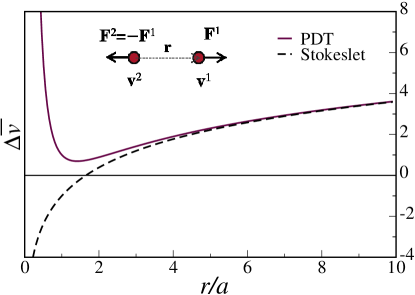
Figure 2: Normalized velocity difference, $\Delta\bar{v}=4\pi\mu\Delta v/F$ ($\Delta v=v^{1}-v^{2}$), of two cylindrical particles of radius $a$, separated by distance $r$ and pulled in opposite directions by forces of the same magnitude $F$, plotted versus the ratio $r/a$. The Stokeslet approximation (dashed black line) yields negative $\Delta v$ (particles move inward while driven outward) at the overlapping distances, $r\lesssim 1.65a$, while the PDT (maroon solid line) gives strictly positive results for all $r/a$ values.

II.2 Test case 2: Ring of normally driven cylinders

We now examine an initial configuration of $N=10$ cylindrical particles evenly distributed along a circular ring of radius $R=1$. The particles are driven in the normal outward direction by identical forces ${\bf F}=F\hat{{\bf n}}$ (see Fig. 3) and interact hydrodynamically. We take $\kappa=10^{-3}$ and $\mu=1$ and check various line fractions $\phi$, such that $a=\phi\pi/N$. At every time-step we calculate the velocity of each particle according to Eq. (20) and advance them to their new positions at the next step. The velocity hardly changes within the considered $50$ steps. We compare the results obtained with and without the correction term (see Fig. 3).

The figure shows that above a certain particle density, $\phi_{c}\simeq 0.55$, the uncorrected tensor yields negative velocities — the ring shrinks under an outward forcing. For the same parameters, the new tensor gives strictly positive velocities — the ring always expands, for all line fractions. As the density increases, the calculated velocities, although positive, become inaccurate. In particular, at $\phi=1$, the velocity is expected to vanish due to the impossibility of inward flow, while the approximate tensor produces a relatively small finite value.

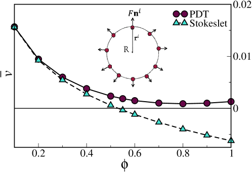
Figure 3: Normalized velocities, $\bar{v}=4\pi\mu v/F$, of $N=10$ cylindrical particles of radius $a$, arranged in a symmetrical ring of radius $R$ and normally driven by a force of magnitude $F$, plotted versus particle density $\phi$ (line fraction). The velocities calculated using the Stokeslet approximation (blue triangles, dashed line) become negative above a certain density $\phi_{c}\simeq 0.55$. The velocities calculated using the positive-definite tensor (maroon circles, solid line) are positive at all densities. The normalized curves depend on $\kappa$ and $N$ only, and we have used $\kappa=10^{-3}$. The value of $a/R$ is set at each point by the density, according to $a/R=\pi\phi/N$.

III Discussion

This work addresses the many-body hydrodynamic interactions among driven or diffusing cylindrical objects within a viscous sheet. Treating two test cases, a pair of particles and a ring of many particles, we have demonstrated the elimination of non-physical situations of negative mobility, using the derived PDT. Therefore, the tensor can be safely used in numerical calculations involving short-range hydrodynamic interactions, such as Stokesian Dynamics schemes Stokesdyn for viscous sheets.

Despite the ensured stability, we stress again that the formalism and the resulting tensor are not exact, but limited to second order in the ratio of particle size to separation. A treatment of many-body dynamics which would be accurate to higher orders, should involve not only the correction to the pair-mobility, but a departure from the pair-wise superposition assumption as well.

One application of the formalism developed here is directly related to the permeability of immobile protein assemblies in membranes to lipid flow. This problem will be discussed in a forthcoming publication. Another example would be an improved calculation of the self-mobility or diffusivity of extended objects, such as rods and polymer molecules, embedded in a viscous sheet or membrane LevineMob ; Noruzifar . We recall that in such calculations, the correction found by Rotne and Prager to the Kirkwood-Riseman tensor vanishes upon spatial averaging, as noted by Yamakawa Yamakawa . The same holds for our correction to the Stokeslet approximation in 2D. Therefore, the preaveraging approximation for extended objects should not be used with the corrected tensor, as it will nullify the effects of the correction term.

An important extension of this work would be to take into consideration viscoelastic (frequency-dependent) effects, either within the sheet Camley2 , or in its surrounding environment Komura .

Appendix A: Tensor derivation based on pair-mobility

In this Appendix we recalculate the corrected pair-mobility of two cylindrical particles following Ref. 9. We show that the many-particle tensor constructed from superposition of these pair-mobilities coincides with the PDT derived in the main text.

The starting point is once again the flow field induced by a single cylinder located at the origin and driven by the force ${\bf F}^{1}$. Our purpose is to calculate the velocity ${\bf v}^{2}({\bf r})$ of another, force-free, cylinder, embedded in this flow field at position ${\bf r}$. For a sphere in a 3D viscous fluid, this relation between the particle velocity ${\bf v}^{2}({\bf r})$ and the flow velocity ${\bf u}({\bf r})$ is given by Faxén’s first law Faxen . The analogous law for a cylinder in a viscous sheet, in the limit $\kappa^{-1}\gg a$, was derived in Ref. 9,

$${\bf v}^{2}({\bf r}) = {\bf u}({\bf r})+\frac{a^{2}}{4}\nabla^{2}{\bf u}.$$ (22)

Substituting Eq. (18) in Eq. (22), we obtain ${\bf v}_{\alpha}^{2}({\bf r})={\bf B}_{\alpha\beta}^{12}({\bf r}){\bf F}_{\beta}^{1}$ with the pair-mobility

$${\bf B}_{\alpha\beta}^{12}=\frac{1}{4\pi\mu}\left[\left(\ln\frac{2}{\kappa r}-\gamma-\frac{1}{2}+\frac{a^{2}}{r^{2}}\right)\boldsymbol{\delta}_{\alpha\beta}+\left(1-\frac{2a^{2}}{r^{2}}\right)\frac{{\bf r}_{\alpha}{\bf r}_{\beta}}{r^{2}}\right].$$ (23)

This result coincides with the pair-mobility block $\bar{{\bf B}}^{i\neq j}_{\alpha\beta}$ of Eq. (20). Hence, the many-particle mobility tensor, constructed from such pair-mobilities, is identical to our PDT. Note, however, that this alternative derivation does not prove positive-definiteness of the constructed tensor.

Appendix B: Overlapping particles

The mobility tensor derived in the main text, Eq. (20), is guaranteed to be positive-definite provided that the disks do not overlap, i.e., $r^{ij}>2a$ for all pairs $i,j$. (Its derivation relied on the flow and stress fields around a single forced disk, which are defined only outside the disk.) This restriction does not pose a problem if short-range repulsion between particles is included, as is done in most simulations. Still, extending the mobility tensor to include overlapping separations may be useful, e.g., in simulations where direct interactions are not of interest. The “inner” tensor (for $r^{ij}\leq 2a$) can be derived by recalculating the integrals in Sec. II while replacing the two circular boundaries of the interacting disks by the boundary of two overlapping disks, as was done for the 3D case in Refs. 16; 35. Here we obtain the inner tensor in a simpler way, by postulating its general form and imposing the conditions that it should satisfy.

Based on the required integrations and the 3D calculation,RP ; Wajnryb2013 we anticipate an inner tensor of the form,

$$\bar{{\bf B}}^{i\neq j}_{\alpha\beta}(r^{ij}\leq 2a)= \frac{1}{4\pi\mu}\left[\left(C_{1}+C_{2}\frac{r^{ij}}{2a}+C_{3}\frac{r^{ij}}{2a}\ln\frac{r^{ij}}{2a}\right)\boldsymbol{\delta}_{\alpha\beta}\right.$$ (24)

$$\left.+\left(D_{1}+D_{2}\frac{r^{ij}}{2a}+D_{3}\frac{r^{ij}}{2a}\ln\frac{r^{ij}}{2a}\right)\frac{{\bf r}^{ij}_{\alpha}{\bf r}^{ij}_{\beta}}{(r^{ij})^{2}}\right].$$

To find the six coefficients we impose the following conditions (satisfied also in the 3D case): (a) the inner tensor should be divergenceless, similar to the outer one; (b) it should converge continuously to the outer tensor at $r^{ij}=2a$; (c) at $r^{ij}=0$, as the two disks overlap perfectly, they move together, i.e., the tensor should converge to $B_{\rm s}\boldsymbol{\delta}_{\alpha\beta}$. These conditions yield,

$$C_{1} = \ln\frac{2}{\kappa a}-\gamma,$$

$$C_{2} = -\ln 2-\frac{1}{4},$$

$$C_{3} = 2\ln 2-\frac{3}{2},$$

$$D_{1} = 0,$$

$$D_{2} = \frac{1}{2},$$

$$D_{3} = -\ln 2+\frac{3}{4}.$$ (25)

Equations (20), (24), and (25), together, give the mobility tensor for disks at all distances, including the possibility of overlap.

Appendix C: Large separations in membranes

In the main text, the tensor of Eq. (20) is limited to particle separations smaller than the cutoff, $r^{ij}\ll\kappa^{-1}$ for all pairs $i,j$. In the particular case of fluid membranes, the cutoff distance, and the hydrodynamic interaction beyond it, are well characterized, arising from the coupling of the membrane to the surrounding 3D fluid. It would be important for large-scale simulations of membrane inclusions to have a mobility tensor which is valid also for $r^{ij}\gtrsim\kappa^{-1}$.

A natural extension of Eq. (20) is the replacement of the logarithmic Green’s function, Eq. (7), by the full Green’s function for a membrane,Naomi ; LevineDyn while keeping the short-range ($\sim a^{2}/r^{2}$) correction terms. This results in

$$\bar{{\bf B}}^{i=j}_{\alpha\beta}= \frac{1}{4\pi\mu}\left(\ln\frac{2}{\kappa a}-\gamma\right)\boldsymbol{\delta}_{\alpha\beta},$$

$$\bar{{\bf B}}^{i\neq j}_{\alpha\beta}(r^{ij})= \frac{1}{4\mu}\left\{\left[H_{0}(\kappa r^{ij})-\frac{H_{1}(\kappa r^{ij})}{\kappa r^{ij}}-\frac{1}{2}\left(Y_{0}(\kappa r^{ij})-Y_{2}(\kappa r^{ij})\right)+\frac{2+a^{2}}{\pi(\kappa r^{ij})^{2}}\right]\boldsymbol{\delta}_{\alpha\beta}\right.$$ (26)

$$-\left.\left[H_{0}(\kappa r^{ij})-\frac{2H_{1}(\kappa r^{ij})}{\kappa r^{ij}}+Y_{2}(\kappa r^{ij})+\frac{2(2+a^{2})}{\pi(\kappa r^{ij})^{2}}\right]\frac{{\bf r}^{ij}_{\alpha}{\bf r}^{ij}_{\beta}}{(r^{ij})^{2}}\right\},$$

where $Y_{n}$ and $H_{n}$ are, respectively, Bessel functions of the second kind and Struve functions. This tensor covers all values of $r^{ij}$, whether smaller or larger than $\kappa^{-1}$, as long as $r^{ij},\kappa^{-1}\gg a$. For separations $r^{ij}\ll\kappa^{-1}$ it coincides with the PDT of Eq. (20), while at larger separations the positiveness issue is irrelevant. Thus, even though we cannot provide a rigorous proof for the positive-definiteness of Eq. (26), this mobility tensor is very plausibly positive-definite for all configurations of membrane inclusions.

References

- (1) P. G. Saffman and M. Delbruck, Proc. Nat. Acad. Sci. USA 72, 3111 (1975).
- (2) V. Prasad and E. R. Weeks, Phys. Rev. E 80, 026309 (2009).
- (3) Z. H. Nguyen, M. Atkinson, C. S. Park, J. Maclennan, M. Glaser, and N. Clark, Phys. Rev. Lett. 105, 268304 (2010).
- (4) Z. Qi, Z. H. Nguyen, C. S. Park, M. A. Glaser, J. E. Maclennan, N. A. Clark, T. Kuriabova, and T. R. Powers, Phys. Rev. Lett. 113, 128304 (2014).
- (5) V. Prasad, S. A. Koehler, and E. R. Weeks, Phys. Rev. Lett. 97, 176001 (2006).
- (6) F. L. H. Brown, Quart. Rev. Biophys. 44, 391 (2011).
- (7) P. G. Saffman, J. Fluid Mech. 73, 593 (1976).
- (8) B. D. Hughes, B. A. Pailthorpe, and L. R. White, J. Fluid Mech. 110, 349 (1981).
- (9) N. Oppenheimer and H. Diamant, Biophys. J. 96, 3041 (2009).
- (10) A. J. Levine and F. C. MacKintosh, Phys. Rev. E 66, 061606 (2002).
- (11) A. J. Levine, T. B. Liverpool, and F. C. MacKintosh, Phys. Rev. E 69, 021503 (2004).
- (12) A. Naji, P. J. Atzberger, and F. L. H. Brown, Phys. Rev. Lett. 102, 138102 (2009).
- (13) B. A. Camley and F. L. H. Brown, Soft Matter 9, 4767 (2013)
- (14) E. Noruzifar, B. A. Camley, and F. L. H. Brown, J. Chem. Phys. 141, 124711 (2014).
- (15) R. Zwanzig, J. Kiefer, and G. H. Weiss, Proc. Natl. Acad. Sci. USA 60, 381 (1968).
- (16) J. Rotne and S. Prager, J. Chem. Phys. 50, 4831 (1969).
- (17) H. Yamakawa, J. Chem. Phys. 53, 436 (1970).
- (18) J. Happel and H. Brenner, Low Reynolds Number Hydrodynamics, Martinus Nijhoff, The Hague, 1983, Sec. 6.2.
- (19) E. Evans and E. Sackmann, J. Fluid Mech. 194, 553 (1988).
- (20) H. A. Stone and A. Ajdari, J. Fluid Mech. 369, 151 (1998).
- (21) A. Naji, A. J. Levine, and P. A. Pincus, Biophys. J. 93, L49 (2007).
- (22) D. R. Daniels and M. S. Turner, Langmuir 23, 6667 (2007).
- (23) M. L. Henle and A. J. Levine, Phys. Rev. E 81, 011905 (2010).
- (24) S. Ramachandran, S. Komura, K. Seki, and G. Gompper, Eur. Phys. J. E 34, 46 (2011).
- (25) C. Pozrikidis, Boundary Integral and Singularity Methods for Linearized Viscous Flow, Cambridge University Press, 1992, Sec. 2.2.
- (26) S. J. Bussell, D. L. Koch, and D. A. Hammer, J. Fluid Mech. 243, 679 (1992).
- (27) D. K. Lubensky and R. E. Goldstein, Phys. Fluids 8, 843 (1996).
- (28) J. G. Kirkwood and J. Riseman, J. Chem. Phys. 16, 565 (1948).
- (29) J. Happel and H. Brenner, Low Reynolds Number Hydrodynamics, Martinus Nijhoff, The Hague, 1983, Sec. 6.4.
- (30) M. Doi, Soft Matter Physics, Oxford University Press, 2013, Chap. 7.
- (31) J. F. Brady, Ann. Rev. Fluid Mech. 20, 111 (1988).
- (32) B. A. Camley and F. L. H. Brown, Phys. Rev. E 84, 021904 (2011).
- (33) S. Komura, S. Ramachandran, and K. Seki, Europhys. Lett. 97, 68007 (2012).
- (34) J. Happel and H. Brenner, Low Reynolds Number Hydrodynamics, Martinus Nijhoff, The Hague, 1983, Sec. 3.2.
- (35) E. Wajnryb, K. A. Mizerski, P. J. Zuk, and P. Szymczak, J. Fluid Mech. 731, R3 (2013).