Which Evaluations Uncover Sense Representations that Actually Make Sense?

Abstract

Text representations are critical for modern natural language processing. One form of text representation, sense-specific embeddings, reflect a word’s sense in a sentence better than single-prototype word embeddings tied to each type. However, existing sense representations are not uniformly better: although they work well for computer-centric evaluations, they fail for human-centric tasks like inspecting a language’s sense inventory. To expose this discrepancy, we propose a new coherence evaluation for sense embeddings. We also describe a minimal model (Gumbel Attention for Sense Induction) optimized for discovering interpretable sense representations that are more coherent than existing sense embeddings.

1 Context, Sense, and Representation

Computers need to represent the meaning of words in context. bert Devlin et al. (2019) and elmo Peters et al. (2018) have dramatically changed how natural language processing represents text. Rather than one-size-fits-all word vectors that ignore the nuance of how words are used in context, these new representations have topped the leaderboards for question answering, inference, and classification.

Contextual representations have supplanted multisense embeddings Camacho-Collados and Pilehvar (2018). While these methods learn a vector for each sense, they do not work encode meanings in downstream tasks as well as contextual representations Peters et al. (2018).

However, computers are not the only consumer of text representations. Humans also use word representations to understand diachronic drift, investigate a language’s sense inventory, or to cluster and explore documents. Thus, a primary role for multisense word embeddings is human understanding of word meanings. Unfortunately, multisense models have only been evaluated on computer-centric dimensions and have ignored the question of sense interpretability.

We first develop measures for how well models encode and explain a word’s meaning to a human (Sec. 4). Existing multisense models do not necessarily fare best on this evaluation; our simpler model (Gumbel Attention for Sense Induction: gasi, Sec. 2) that focuses on discrete sense selection can better capture human-interpretable representations of senses; comparing against traditional evaluations (Sec. 5), gasi has better contextual word similarity and competitive non-contextual word similarity. Finally, we discuss the connections between representation learning and how modern contextual representations could better capture interpretable senses (Sec. 6).

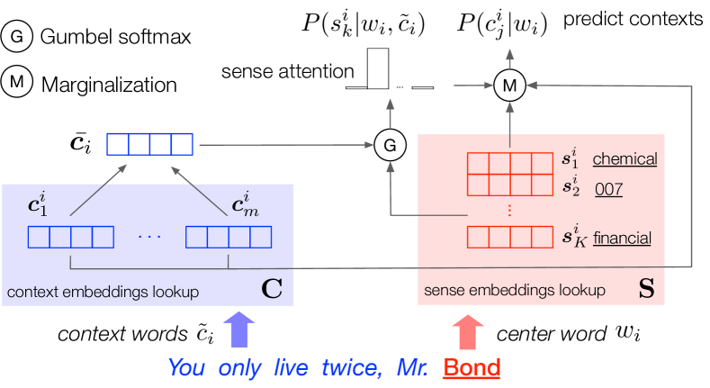
Figure 1: Network structure with an example of our gasi model which learns a set of global context embeddings C and a set of sense embeddings S.

2 Attentional Sense Induction

Before we explore human interpretability of sense induction, we first describe our simple models to disentangle word senses. Our two models are built on Word2Vec (Mikolov et al., 2013a, b), which we review in Sec. 2.1. Both models use a straightforward attention mechanism to select which sense is used in a token’s context, which we contrast to alternatives for sense selection (Sec. 2.3). Building on these foundations, we introduce our model, gasi, and along the way introduce a soft-attention stepping-stone (sasi).

2.1 Foundations: Skip-Gram and Gumbel

Word2Vec jointly learns word embeddings $\text{{W}}\in\mathbb{R}^{|V|\times d}$ and context embeddings $\text{{C}}\in\mathbb{R}^{|V|\times d}$. More specifically, given a vocabulary $V$ and embedding dimension $d$, it maximizes the likelihood of the context words $c_{j}^{i}$ that surround a given center word $w_{i}$ in a context window $\tilde{c}_{i}$,

$$J(\text{{W}},\text{{C}})\propto\sum_{w_{i}\in V}\sum_{c_{j}^{i}\in\tilde{c}_{i}}\log P(c_{j}^{i}\,|\,w_{i};\text{{W}},\text{{C}}),$$ (1)

where $P(c_{j}^{i}\,|\,w_{i})$ is over the vocabulary,

$$P(c_{j}^{i}\,|\,w_{i};\text{{W}},\text{{C}})=\frac{\exp\left({\bm{c}_{j}^{i}}^{\top}\bm{w}_{i}\right)}{\sum_{c\in V}\exp\left(\bm{c}^{\top}\bm{w}_{i}\right)}.$$ (2)

In practice, $\log P(c_{j}^{i}\,|\,w_{i})$ is approximated by negative sampling. We extend it to learn representations for individual word senses.

2.2 Gumbel Softmax

As we introduce word senses, our model will need to select which sense is relevant for a context. The Gumbel softmax (Jang et al., 2016; Maddison et al., 2016) approximates the sampling of discrete random variables; we use it to select the sense. Given a discrete random variable $X$ with $P(X=k)\propto\alpha_{k}$, $\alpha_{k}\in(0,\infty)$, the Gumbel-max (Gumbel and Lieblein, 1954) refactors the sampling of $X$ into

$$X=\operatorname*{arg\,max}_{k}(\log\alpha_{k}+g_{k}),$$ (3)

where the Gumbel noise $g_{k}=-\log(-\log(u_{k}))$ and $u_{k}$ are i.i.d. from Uniform(0, 1). The Gumbel softmax approximates sampling $\operatorname{one\_hot}(\operatorname*{arg\,max}_{k}(\log\alpha_{k}+g_{k}))$ by

$$y_{k}=\operatorname{softmax}((\log\alpha_{k}+g_{k})/\tau).$$ (4)

Unlike soft selection of senses, the Gumbel softmax can make harder selections, which will be more interpretable to humans.

2.3 Why Attention? Musing on Alternatives

For fine-grained sense inventories, it makes sense to have graded assignment of tokens to senses Erk et al. (2009); Jurgens and Klapaftis (2015). However, for coarse senses—except for humor Miller et al. (2017)—words typically are associated with a single sense, often a single sense per discourse Gale et al. (1992). A good model should respect this. Previous models either use non-differentiable objectives or—in the case of the current state of the art, muse Lee and Chen (2017)—reinforcement learning to select word senses. By using Gumbel softmax, our model both approximates discrete sense selection and is differentiable.

As we argue in the next section, applications with a human in the loop are best assisted by discrete senses; the Gumbel softmax, which we develop for our task here, helps us discover these discrete senses.

2.4 Attentional Sense Induction

Embeddings

We learn a context embedding matrix $\text{{C}}\in\mathbb{R}^{|V|\times d}$ and a sense embedding tensor $\text{{S}}\in\mathbb{R}^{|V|\times K\times d}$. Unlike previous work (Neelakantan et al., 2014; Lee and Chen, 2017), no extra embeddings are kept for sense induction.

Number of Senses

For simplicity and consistency with previous work, our model has $K$ fixed senses. Ideally, if we set a large number of $K$, with a perfect pruning strategy, we can estimate the number of senses per type by removing duplicated senses.

However, this is challenging McCarthy et al. (2016); instead we use a simple pruning strategy. We estimate a pruning threshold $\lambda$ by averaging the estimated duplicate sense and true neighbor distances,

$$\lambda=\frac{1}{2}(\operatorname{mean}(D_{dup})+\operatorname{mean}(D_{nn})),$$ (5)

where $D_{dup}$ are the cosine distances for duplicated sense pairs and $D_{nn}$ is that of true neighbors (different types). We sample 100 words and if two senses are top-5 nearest neighbors of each other, we consider them duplicates.

After pruning duplicated senses with $\lambda$, we can retrain a new model with estimated number of senses for each type by masking the sense attentions. Results in Table 2 and 5 validate our pruning strategy.

Sense Attention in Objective Function

Assuming a center word $w_{i}$ has senses $\{s_{1}^{i},s_{2}^{i},\dots,s_{K}^{i}\}$, the original Skip-Gram likelihood becomes a marginal distribution over all senses of $w_{i}$ with sense induction probability $P(s_{k}^{i}\,|\,w_{i})$; we focus on the disambiguation given local context $\tilde{c}_{i}$ and estimate $P(s_{k}^{i}\,|\,w_{i})\approx P(s_{k}^{i}\,|\,w_{i},\tilde{c}_{i})$; and thus,

$$P(c_{j}^{i}\,|\,w_{i})\approx\sum_{k=1}^{K}P(c_{j}^{i}\,|\,s_{k}^{i})\underbrace{P(s_{k}^{i}\,|\,w_{i},\tilde{c}_{i})}_{\mbox{{attention}}},$$ (6)

Replacing $P(c_{j}^{i}\,|\,w_{i})$ in Equation 1 with Equation 6 gives our objective function $J(\text{{S}},\text{{C}})\propto$

$$\sum_{w_{i}\in V}\sum_{c_{j}^{i}\in\tilde{c}_{i}}\log\sum_{k=1}^{K}P(c_{j}^{i}\,|\,s_{k}^{i})P(s_{k}^{i}\,|\,w_{i},\tilde{c}_{i}).$$ (7)

Modeling Sense Attention

We can model the contextual sense induction distribution with soft attention; we call the resulting model soft-attention sense induction (sasi); although it is a stepping stone to our final model, we compare against it in our experiments as it isolates the contributions of hard attention. In sasi, the sense attention is conditioned on the entire local context $\tilde{c}_{i}$ with softmax:

$$P(s_{k}^{i}\,|\,w_{i},\tilde{c}_{i})=\frac{\exp\left(\bar{\bm{c}}_{i}^{\top}\bm{s}_{k}^{i}\right)}{\sum_{k=1}^{K}\exp\left(\bar{\bm{c}}_{i}^{\top}\bm{s}_{k}^{i}\right)},$$ (8)

where $\bar{\bm{c}}_{i}$ is the mean of the context vectors in $\tilde{c}_{i}$. A derivation of how this affects negative sampling is in Appendix A.

2.5 Scaled Gumbel Softmax for Sense Disambiguation

To learn distinguishable sense representations, we implement hard attention in our full model, Gumbel Attention for Sense Induction (gasi). While hard attention is conceptually attractive, it can increase computational difficulty: discrete choices are not differentiable and thus incompatible with modern deep learning frameworks. To preserve differentiability (and resorting to equally complex reinforcement learning), we apply the Gumbel softmax reparameterization trick to our sense attention function (Equation 8).

Vanilla Gumbel

The discrete sense sampling from Equation 8 can be refactored

$$\bm{z^{i}}=\operatorname{one\_hot}(\operatorname*{arg\,max}_{k}(\bar{\bm{c}_{i}}^{\top}\bm{s}_{k}^{i}+g_{k})),$$ (9)

and the hard attention approximated

$$y_{k}^{i}=\operatorname{softmax}((\bar{\bm{c}_{i}}^{\top}\bm{s}_{k}^{i}+g_{k})/\tau).$$ (10)

Scaled Gumbel

Gumbel softmax learns a flat distribution over senses even with low temperatures: the dot product $\bar{\bm{c}}_{i}^{\top}\bm{s}_{k}^{i}$ is too small compared to the Gumbel noise $g_{k}$. Thus we use a scaling factor $\beta$ to encourage sparser distributions,

$$\gamma_{k}^{i}=\operatorname{softmax}((\bar{\bm{c}_{i}}^{\top}\bm{s}_{k}^{i}+\beta g_{k})/\tau),$$ (11)

and tune it as a hyperparameter. We append gasi-$\beta$ to the name of models with a scaling factor. This is critical for learning distinguishable senses (Figure 2, Table 5, and Table 2). Our final objective function for gasi-$\beta$ is

$$J(\text{{S}},\text{{C}})\propto\sum_{w_{i}\in V}\sum_{w_{c}\in c_{i}}\sum_{k=1}^{K}\gamma_{k}^{i}\log P(w_{c}\,|\,s_{k}^{i}).$$ (12)

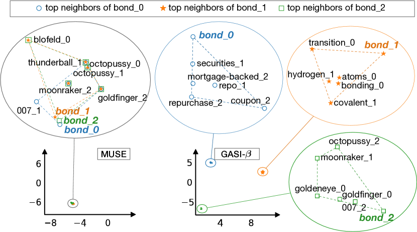
Figure 2: t-sne projections of nearest neighbors for “bond” by hard-attention models: muse (rl-based) and our gasi-$\beta$. Trained on same dataset and vocabulary, both models learn three vectors per word (bond$\_i$ is $i$^th sense vector). gasi (right) learns three distinct senses of “bond” while muse (left) learns overlapping senses.

3 Data and Training

For fair comparisons, we try to remain consistent with previous work (Huang et al., 2012; Neelakantan et al., 2014; Lee and Chen, 2017) in all aspects of training. In particular, we train gasi on the same April 2010 Wikipedia snapshot (Shaoul C., 2010) with 1B tokens and the same vocabulary released by Neelakantan et al. (2014); set the number of senses $K=3$ and dimension $d=300$ for each word unless otherwise specified. More details are in the Appendix. Following Maddison et al. (2016), we fix the temperature $\tau=0.5$, and tune the scaling factor $\beta=0.4$ using grid search within $\{0.1\dots 0.9\}$ on AvgSimC for contextual word similarity (Section 5); this tuning preceded all interpretability experiments. If not reprinted, numbers for competing models are either computed with pre-trained embeddings released by authors or trained on released code.

4 Evaluating Interpretability

We turn to traditional evaluations of sense embeddings later (Section 5), but our focus is on human interpretability. If you show a human the senses, can they understand why a model would assign a sense to that context? This section evaluates whether the representations make sense to human consumers of multisense models.

In the age of bert and elmo, these are the dimensions that are most critical for multisense representations. While contextual word vectors are most useful for computer understanding of meaning, humans often want an overview of word meanings for other tasks.

Sense representations are useful for human-in-the-loop applications. They help understand semantic drift Hamilton et al. (2016): how do the meanings of “gay” reflect social progress? They help people learn languages Noraset et al. (2017): what does it mean when someone says that I “embarrassed” them? They help linguists understand the sense inventory of a language Kawahara et al. (2014): what are the frames that can be used by the verb “participate”? These questions (and human understanding) are helped by discrete senses, which the Gumbel softmax uncovers.

More broadly, this is the goal of interpretable machine learning Doshi-Velez and Kim (2017). While downstream models do not always need an interpretable explanation of why a model uses a particular representation, interactive machine learning and explainable machine learning do. To date, multisense representations ignore this use case.

Model	Sense	Judgment	Agreement
	Accuracy	Accuracy
muse	67.33	62.89	0.73
mssg-30k	69.33	66.67	0.76
gasi-$\beta$	71.33	67.33	0.77

Table 1: Word intrusion evaluations on top ten nearest neighbors of sense embeddings. Users find misfit words most easily with gasi-$\beta$, suggesting these representations are more interpretable.

Qualitative analysis

Previous papers use nearest neighbors of a few examples to qualitatively argue that their models have captured meaningful senses of words. We also give an example in Figure 2, which provides an intuitive view on how the learned senses are clustered by visualizing the nearest neighbors of word “bond” using t-sne projection (Maaten and Hinton, 2008). Our model (right) disentangles the three sense of “bond” clearly.

However, examples can be cherry-picked. This problem bedeviled topic modeling until rigorous human evaluation was introduced (Chang et al., 2009). We adapt both aspects of their evaluations: word intrusion (Schnabel et al., 2015) to evaluate whether individual senses are coherent and topic intrusion—rather sense intrusion in this setting—to evaluate whether humans agree with models’ sense assignments in context. Using crowdsourced evaluations from Figure-Eight, we compare our models with two previous state-of-the-art sense embeddings models, i.e., mssg (Neelakantan et al., 2014) and muse (Lee and Chen, 2017).

Model	Accuracy	$P$	Agreement
muse	28.0	0.33	0.68
mssg-30K	44.5	0.37	0.73
gasi (no $\beta$)	33.8	0.33	0.68
gasi-$\beta$	50.0	0.48	0.75
gasi-$\beta$-pruned	75.2	0.67	0.96

Table 2: Human-model consistency on contextual word sense selection; $P$ is the average probability assigned by the model to the human choices. gasi-$\beta$ is most consistent with crowdworkers. Reducing sense duplications by retraining our model with pruning mask improves significantly human-model agreement.

4.1 Word Intrusion for Sense Coherence

Schnabel et al. (2015) suggest a “good” word embedding should have coherent neighbors and evaluate coherence by word intrusion. They present crowdworkers four words: three are close in embedding space while one of which is an “intruder”. If the embedding makes sense, contributors will easily spot the word that “does not belong”.

Similarly, we examine the coherence of ten nearest neighbors of senses in the contextual word sense selection task (Section 4.2) and replace one neighbor with an “intruder”. We generate three intruders for each sense and collect three judgments per intruder. To account for variation in users and intruders, we count an instance as “correct” if two or more crowdworkers correctly spot the intruder.

Like Chang et al. (2009), we want the “intruder” to be about as frequent as the target but not too similar. For sense $s_{i}^{m}$ of word type $w_{i}$, we randomly select a word from the neighbors of another sense $s_{i}^{n}$ of $w_{i}$.

All models have comparable model accuracy. gasi-$\beta$ learns senses that have the highest coherence while muse learns mixtures of senses (Table 1).

We use the aggregated confidence score provided by Figure-Eight to estimate the level of inter-rater agreement between multiple contributors Figure Eight (2018). The agreement is high for all models and gasi-$\beta$ has the highest agreement, suggesting that the senses learned by gasi-$\beta$ are easier to interpret.

4.2 Contextual Word Sense Selection

The previous task measures whether individual senses are coherent. Now we evaluate models’ disambiguation of senses in context.

Task Description

Given a target word in context, we ask a crowdworker to select which sense group best fits the sentence. Each sense group is described by its top ten distinct nearest neighbors, and the sense group order is shuffled.

Data Collection

We select fifty nouns with five sentences from SemCor 3.0 (Miller et al., 1994). We first filter all word types with fewer than ten sentences and select the fifty most polysemous nouns from WordNet (Miller and Fellbaum, 1998) among the remaining senses. For each noun, we randomly select five sentences.

Metrics

For each model, we collect three judgments for each question. We consider a model correct if at least two crowdworkers select the same sense as the model.

		muse	mssg	gasi-$\beta$
word overlap	agree	4.78	0.39	1.52
	disagree	5.43	0.98	6.36
Glove cosine	agree	0.86	0.33	0.36
	disagree	0.88	0.57	0.81

Table 3: Similarities of human and model choices when they agree and disagree for two metrics: simple word overlap (top) and Glove cosine similarity (bottom). Humans agree with the model when the senses are distinct.

The real question is - how are those four years used and what is their value as training?
s1	hypothetical, unanswered, topic, answered, discussion, yes/no, answer, facts
s2	toss-up, answers, guess, why, answer, trivia, caller, wondering, answering
s3	argument, contentious, unresolved, concerning, matter, regarding, debated, legality

Table 4: A case where mssg has low overlap but confuses raters (agreement 0.33); model chooses s1.

Sense Disambiguation and Interpretability

If humans consistently pick the same sense as the model, they must first understand the choices, thus implying the nearest neighbor words were coherent. Moreover, they also agree that among those senses, that sense was the right choice for this token. gasi-$\beta$ selections are most consistent with humans’; it has the highest accuracy and assigns the largest probability assigned to the human choices (Table 2). Thus, gasi-$\beta$ produces sense embeddings that are both more interpretable and distinguishable. gasi without a scaling factor, however, has low consistency and flat sense distribution.

Model Confidence

However, some contexts are more ambiguous than others. For fine-grained senses, best practice is to use graded sense assignments Erk et al. (2013). Thus, we also show the model’s probability of the top human choice; distributions close to $\frac{1}{K}$ (0.33) suggest the model learns a distribution that cannot disambiguate senses. We consider granularity of senses further in Sec. 6.

Inter-rater Agreement

We use the confidence score computed by Figure-Eight to estimate the raters’ agreement for this task. gasi-$\beta$ has the highest human-model agreement, while both Muse and gasi without scaling have the lowest.

Error Analysis

Next, we explore why crowdworkers disagree with the model even though the senses are interpretable (Table 1). Is it that the model has learned duplicate senses that both the users and model cannot distinguish (the senses are all bad or identical) or is it that crowdworkers agree with each other but disagree with the model (the model selects bad senses)?

Two trends suggest duplicate senses cause disagreement both for humans with models and humans with each other. For two measures of sense similarity—simple word overlap and glove similarity—similarity is lower when users and models agree (Table 3). Humans also agree with each other more. For gasi-$\beta$, pairs with perfect agreement have a word overlap of around 2.5, while the senses with lowest agreement have overlap around 5.5.

To reduce duplicated senses, we retrain the model with pruning (Section 2.4, Equation 5). We remove a little more than one sense per type on average. To maintain the original setting, for word types that have fewer than three senses left, we compute the nearest neighbors to dummy senses represented by random embeddings. Our model trained with pruning mask (gasi-$\beta$-pruned) reaches very high inter-rater agreement and higher human-model agreement than models with a fixed number of senses (Table 2, bottom).

5 Word Similarity Evaluation

gasi and gasi-$\beta$ are interpretable, but how do they fare on standard word similarity tasks?

Contextual Word Similarity

Tailored for sense embedding evaluation, Stanford Contextual Word Similarities (Huang et al., 2012, scws) has 2003 word pairs tied to context sentences. These tasks assign a pair of word types (e.g., “green” and “buck”) a similarity/relatedness score. Moreover, both words in the pair have an associated context. These contexts disambiguate homonymous and polysemous word types and thus captures sense-specific similarity. Thus, we use this dataset to tune our hyperparameters, comparing Spearman’s rank correlation $\rho$ between embedding similarity and the gold similarity judgments: higher scores imply the model captures semantic similarities consistent with the trusted similarity scores.

To compute the word similarity with senses we use two metrics Reisinger and Mooney (2010) that take context and sense disambiguation into account: MaxSimC computes the cosine similarity $\cos(s_{1}^{*},s_{2}^{*})$ between the two most probable senses $s_{1}^{*}$ and $s_{2}^{*}$ that maximizes $P(s_{k}^{i}\,|\,w_{i},\tilde{c}_{i})$. AvgSimC weights average similarity over the combinations of all senses $\sum_{i=1}^{K}\sum_{i=j}^{K}P(s_{i}^{1}\,|\,w_{1},\tilde{c}_{1})P(s_{j}^{2}\,|\,w_{2},\tilde{c}_{2})\cos(s_{i}^{1}s_{j}^{2})$.

We compare variants of our model with existing sense embedding models (Table 5), including two previous sotas: the clustering-based Multi-Sense Skip-Gram model (Neelakantan et al., 2014, mssg) on AvgSimC and the rl-based Modularizing Unsupervised Sense Embeddings (Lee and Chen, 2017, muse) on MaxSimC. gasi better captures similarity than sasi, corroborating that hard attention aids word sense selection. gasi without scaling has the best MaxSimC; however, it learns a flat sense distribution (Figure 2). gasi-$\beta$ has the best AvgSimC and a competitive MaxSimC. While muse has a higher MaxSimC than gasi-$\beta$, it fails to distinguish senses as well (Figure 2, Section 4).

We also evaluate the retrained model with pruning mask on this dataset. gasi-$\beta$-pruned has the same AvgSimC as gasi-$\beta$ and higher local similarity correlation (Table 5, bottom), validating our pruning strategy (Section 2.4).

Model	MaxSimC	AvgSimC
Huang et al. (2012)-50d	26.1	65.7
mssg-6k	57.3	69.3
mssg-30k	59.3	69.2
Tian et al. (2014)	63.6	65.4
Li and Jurafsky (2015)	66.6	66.8
Qiu et al. (2016)	64.9	66.1
Bartunov et al. (2016)	53.8	61.2
muse_Boltzmann	67.9	68.7
sasi	55.1	67.8
gasi (w/o scaling)	68.2	68.3
gasi-$\beta$	66.4	69.5
gasi-$\beta$-pruned	67.0	69.5

Table 5: Spearman’s correlation $100\rho$ on scws (trained on 1B token, 300d vectors except for Huang et al.). gasi and gasi-$\beta$ both can disambiguate the sense and correlate with human ratings. Retraining the model with pruned senses furthur improves local similarity correlation.

Word Sense Selection in Context

scws evaluates models’ sense selection indirectly. We further compare gasi-$\beta$ with previous sota, mssg-30k and muse, on the Word in Context dataset (Pilehvar and Camacho-Collados, 2018, wic) which requires the model to identify whether a word has the same sense in two contexts. To reduce the variance in training and to focus on evaluating the sense selection module, we use an evaluation suited for unsupervised models: if the model selects different sense vectors given contexts, we mark that the word has different senses. For muse, mssg and gasi-$\beta$, we use each model’s sense selection module; for DeConf (Pilehvar and Collier, 2016) and sw2v (Mancini et al., 2017), we follow Pilehvar and Camacho-Collados (2018) and Pelevina et al. (2016) by selecting the closest sense vectors to the context vector. DeConf results are comparable to supervised results (59.4$\pm$ 0.7). gasi-$\beta$ has the best result (55.3) apart from DeConf itself (58.55)(full results in Table 8 in appendix), which uses the same sense inventory (Miller and Fellbaum, 1998, WordNet) as wic.

Non-Contextual Word Similarity

While contextual word similarity is best suited for our model and goals, other datasets without contexts (i.e., only word pairs and a rating) are both larger and ubiquitous for word vector evaluations. To evaluate the semantics captured by each sense-specific embeddings, we compare the models on non-contextual word similarity datasets. Like Lee and Chen (2017) and Athiwaratkun et al. (2018), we compute the word similarity based on senses by MaxSim (Reisinger and Mooney, 2010), which maximizes the cosine similarity over the combination of all sense pairs and does not require local contexts,

$$\text{MaxSim}(w_{1},w_{2})=\max_{0\leq i\leq K,0\leq j\leq K}\cos(s_{i}^{1},s_{j}^{2}).$$ (13)

gasi-$\beta$ has better correlation on three datasets, is competitive on the rest (Table 6), and remains competitive without scaling. gasi is better than muse, the other hard-attention multi-prototype model, on six datasets and worse on three. Our model can reproduce word similarities as well or better than existing models through our sense selection.

Dataset	muse	sasi	gasi	gasi-$\beta$	PFT-GM
SimLex-999	39.61	31.56	40.14	41.68	40.19
WS-353	68.41	58.31	68.49	69.36	68.6
MEN-3k	74.06	65.07	73.13	72.32	77.40
MC-30	81.80	70.81	82.47	85.27	74.63
RG-65	81.11	74.38	77.19	79.77	79.75
YP-130	43.56	48.28	49.82	56.34	59.39
MT-287	67.22	64.54	67.37	66.13	69.66
MT-771	64.00	55.00	66.65	66.70	68.91
RW-2k	48.46	45.03	47.22	47.69	45.69

Table 6: Spearman’s correlation on non-contextual word similarity (MaxSim). gasi-$\beta$ has higher correlation on three datasets and is competitive on the others. pft-gm is trained with two components/senses while other models learn three. A full version including mssg is in appendix.

5.1 Word Similarity vs. Interpretability

Word similarity tasks (Section 5) and human evaluations (Section 4) are inconsistent. gasi, gasi-$\beta$ and muse are all competitive in word similarity (Table 5 and Table 6), but only gasi-$\beta$ also does well in the human evaluations (Table 2). Both gasi without scaling and muse fail to learn distinguishable senses and cannot disambiguate senses. High word similarities do not necessarily indicate “good” sense embeddings quality; our human evaluation—contextual word sense selection—is complementary.

6 Related Work: Representation, Evaluation

Schütze (1998) introduces context-group discrimination for senses and uses the centroid of context vectors as a sense representation. Other work induces senses by context clustering (Purandare and Pedersen, 2004) or probabilistic mixture models (Brody and Lapata, 2009). Reisinger and Mooney (2010) first introduce multiple sense-specific vectors for each word, inspiring other multi-prototype sense embedding models. Generally, to address polysemy in word embeddings, previous work trains on annotated sense corpora (Iacobacci et al., 2015) or external sense inventories (Labutov and Lipson, 2013; Chen et al., 2014; Jauhar et al., 2015; Chen et al., 2015; Wu and Giles, 2015; Pilehvar and Collier, 2016; Mancini et al., 2017); Rothe and Schütze (2017) extend word embeddings to lexical resources without training; others induce senses via multilingual parallel corpora (Guo et al., 2014; Šuster et al., 2016; Ettinger et al., 2016).

We contrast our gasi to unsupervised monolingual multi-prototype models along two dimensions: sense induction methodology and differentiability.

On the dimension of sense induction methodology, Huang et al. (2012) and Neelakantan et al. (2014) induce senses by context clustering; Tian et al. (2014) model a corpus-level sense distribution; Li and Jurafsky (2015) model the sense assignment as a Chinese Restaurant Process; Qiu et al. (2016) induce senses by minimizing an energy function on a context-depend network; Bartunov et al. (2016) model the sense assignment as a steak-breaking process; Nguyen et al. (2017) model the sense embeddings as a weighted combination of topic vectors with pre-computed weights by topic models; Athiwaratkun et al. (2018) model word representations as Gaussian Mixture embeddings where each Gaussian component captures different senses; Lee and Chen (2017) compute sense distribution by a separate set of sense induction vectors. The proposed gasi marginalizes the likelihood of contexts over senses and induces senses by local context vectors; the most similar sense selection module is a bilingual model (Šuster et al., 2016) except that it does not introduce lower bound for negative sampling but uses weighted embeddings, which results in mixed senses.

On the dimension of differentiability, most sense selection models are non-differentiable and discretely select senses, with two exceptions: Šuster et al. (2016) use weighted vectors over senses; Lee and Chen (2017) implement hard attention with rl to mitigate the non-differentiability. In contrast, gasi keeps full differentiability by reparameterization and approximates discrete sense sampling with the scaled Gumbel softmax.

However, the elephants in the room are bert and elmo. While there are specific applications where humans might be better served by multisense embeddings, computers seem to be consistently better served by contextual representations. A natural extension is to use the aggregate representations of word senses from these models. Particularly for elmo, one could cluster individual mentions Chang (2019), but this is unsatisfying at first blush: it creates clusters more specific than senses. bert is even more difficult: the transformer is a dense, rich representation, but only a small subset describes the meaning of individual words. Probing techniques Perone et al. (2018) could help focus on semantic aspects that help humans understand word usage.

6.1 Granularity

Despite the confluence of goals, there has been a disappointing lack of cross-fertilization between the traditional knowledge-based lexical semantics community and the representation-learning community. We, following the trends of sense learning models, have—from the perspective of those used to VerbNet or WordNet—used far too few senses per word. While there is disagreement about sense inventory, “hard” and “line” Leacock et al. (1998) definitely have more than three senses. Expanding to granular senses presents both challenges and opportunities for future work.

While moving to a richer sense inventory is valuable future work, it makes human annotation more difficult Erk et al. (2013)—while we can expect humans to agree on which of three senses are used, we cannot for larger sense inventories. In topic models, Chang et al. (2009) develop topic log odds (in addition to the more widely used model precision) to account for graded assignment to topics. Richer user models would need to capture these more difficult decisions.

However, moving to more granular senses requires richer modeling. Bayesian nonparametrics (Orbanz and Teh, 2010) can determine the number of clusters that best explain the data. Combining online stick breaking distributions Wang et al. (2011) with gasi’s objective function could remove unneeded complexity for word types with few senses and consider the richer sense inventory for other words.

7 Conclusion

The goal of multi-sense word embeddings is not just to win word sense evaluation datasets. Rather, they should also describe language: given millions of tokens of a language, what are the patterns in the language that can help a lexicographer or linguist in day-to-day tasks like building dictionaries or understanding semantic drift. Our differentiable Gumbel Attention Sense Induction (gasi) offers comparable word similarities with multisense representations while also learning more distinguishable, interpretable senses.

However, simply asking whether word senses look good is only a first step. A sense induction model designed for human use should be closely integrated into that task. While we use a Word2Vec-based objective function in Section 2, ideally we should use a human-driven, task-specific metric (Feng and Boyd-Graber, 2019) to guide the selection of senses that are distinguishable, interpretable, and useful.

Appendix

Equation and figure numbers continue from main submission.

A Derivation Desiderata

Like the Skip-Gram objective (Equation 2), we model the likelihood of a context word given the center sense $P(c_{j}^{i}\,|\,s_{k}^{i})$ using softmax,

$$P(c_{j}^{i}\,|\,s_{k}^{i})=\frac{\exp\left({\bm{c}_{j}^{i}}^{\top}\bm{s}_{k}^{i}\right)}{\sum_{j=1}^{|V|}\exp\left(\bm{c}_{j}^{\top}\bm{s}_{k}^{i}\right)},$$ (14)

where the bold symbol $\bm{s}_{k}^{i}$ is the vector representation of sense $s_{k}^{j}$ from S, and $\bm{c}_{j}$ is the context embedding of word $c_{j}$ from C.

Computing the softmax over the vocabulary is time-consuming. We want to adopt negative sampling to approximate $\log P(c_{j}^{i}\,|\,s_{k}^{i})$, which does not exist explicitly in our objective function (Equation 7).

However, given the concavity of the logarithm function, we can apply Jensen’s inequality,

$$\log \left[\sum_{k=1}^{K}P(c_{j}^{i}\,|\,s_{k}^{i})P(s_{k}^{i}\,|\,w_{i},\tilde{c}_{i})\right]\geq$$ (15)

$$\sum_{k=1}^{K}P(s_{k}^{i}\,|\,w_{i},\tilde{c}_{i})\log P(c_{j}^{i}\,|\,s_{k}^{i}),$$

and create a lower bound of the objective. Maximizing this lower bound gives us a tractable objective, $J(\text{{S}},\text{{C}})\propto$

$$\sum_{w_{i}\in V}\sum_{c_{j}^{i}\in\tilde{c}_{i}}\sum_{k=1}^{K}P(s_{k}^{i}\,|\,w_{i},\tilde{c}_{i})\log P(c_{j}^{i}\,|\,s_{k}^{i}),$$ (16)

where $\log P(c_{j}^{i}\,|\,s_{k}^{i})$ is estimated by negative sampling Mikolov et al. (2013b),

$$\text{log }\sigma({\bm{c}_{j}^{i}}^{\top}\bm{s}_{k}^{i})+\sum_{j=1}^{n}\mathbb{E}_{c_{j}\sim P_{n}(c)}[\text{log }\sigma(-\bm{c}_{j}^{\top}\bm{s}_{k}^{j}))]$$

B Training Details

During training, we fix the window size to five and the dimensionality of the embedding space to 300 for comparison to previous work. We initialize both sense and context embeddings randomly within U(-0.5/dim, 0.5/dim) as in Word2Vec. We set the initial learning rate to 0.01; it is decreased linearly until training concludes after 5 epochs. The batch size is 512, and we use five negative samples per center word-context pair as suggested by Mikolov et al. (2013a). The subsample threshold is 1e-4. We train our model on the GeForce GTX 1080 Ti, and our implementation (using pytorch 3.0) takes $\sim 6$ hours to train one epoch on the April 2010 Wikipedia snapshot Shaoul C. (2010) with 100k vocabulary. For comparison, our implementation of Skip-Gram on the same framework takes $\sim 2$ hours each epoch.

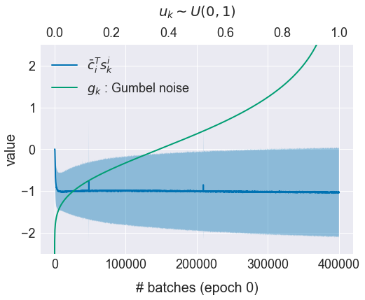
Figure 3: Our hard attention mechanism is approximated with Gumbel softmax on the context-sense dot product $\bar{\bm{c}}_{i}^{\top}\bm{s}_{k}^{i}$ (Equation 10), whose mean and std plotted here as a function of iteration. The shadowed area shows that it has a smaller scale than the Gumbel noise $g_{k}$, such that $g_{k}$, rather than the embeddings, dominates the sense attention.

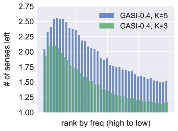
Figure 4: Histogram of number of senses left after post-training pruning for two models: gasi-0.4 initialized with three senses and gasi-0.4 initialized with five senses. We rank the number of senses of words by their frequency from high to low.

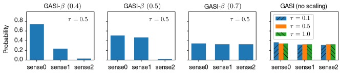
Figure 5: As the scale factor $\beta$ increases, the sense selection distribution for “bond” given examples from SemCor 3.0 for synset “bond.n.02” becomes flatter, indicating less disambiguated sense vectors.

Dataset	mssg-30k	mssg-6k	muse_Boltzmann	sasi	gasi	gasi-$\beta$	PFT-GM
SimLex-999	31.80	28.65	39.61	31.56	40.14	41.68	40.19
WS-353	65.69	67.42	68.41	58.31	68.49	69.36	68.6
MEN-3k	65.99	67.10	74.06	65.07	73.13	72.32	77.40
MC-30	67.79	76.02	81.80	70.81	82.47	85.27	74.63
RG-65	73.90	64.97	81.11	74.38	77.19	79.77	79.75
YP-130	40.69	42.68	43.56	48.28	49.82	56.34	59.39
MT-287	65.47	64.04	67.22	64.54	67.37	66.13	69.66
MT-771	61.26	58.83	64.00	55.00	66.65	66.70	68.91
RW-2k	42.87	39.24	48.46	45.03	47.22	47.69	45.69

Table 7: Spearman’s correlation $100\rho$ on non-contextual word similarity (MaxSim). gasi-$\beta$ outperforms the other models on three datasets and is competitive on others. pft-gm is trained with two components/senses while other models learn three.

C Number of Senses

For simplicity and consistency with most of previous work, we present our model with a fixed number of senses $K$.

C.1 Post-training Pruning and Retraining

For words that do not have multiple senses or have most senses appear very low-frequently in corpus, our model (as well as many previous models) learns duplicate senses. Ideally, if we set a large number of $K$, with a perfect pruning strategy, we can estimate the number of senses per type by removing duplicated senses and retrain a new model with the estimated number of senses instead of a fixed number $K$.

However, this is challenging McCarthy et al. (2016); instead we use a simple pruning strategy and remove duplicated senses with a threshold $\lambda$. Specifically, for each word $w_{i}$, if the cosine distance between any of its sense embeddings ($\bm{s}_{m}^{i},\bm{s}_{n}^{i}$) is smaller than $\lambda$, we consider them to be duplicates. After discovering all duplicate pairs, we start pruning with the sense $s_{k}^{i}$ that has the most duplications and keep pruning with the same strategy until no more duplicates remain.

Model-specific pruning

We estimate a model-specific threshold $\lambda$ from the learned embeddings instead of deciding it arbitrary. We first sample 100 words from the negative sampling distribution over the vocabulary. Then, we retrieve the top-5 nearest neighbors (from all senses of all words) to each sense of each sampled word. If one of a word’s own senses appears as a nearest neighbor, we append the distance between them to a sense duplication list $D_{dup}$. For other nearest neighbors, we append their distances to the word neighbor list $D_{nn}$. After populating the two lists, we want to choose a threshold that would prune away all of the sense duplicates while differentiating sense duplications with other distinct neighbor words. Thus, we compute

$$\lambda=\frac{1}{2}(\operatorname{mean}(D_{dup})+\operatorname{mean}(D_{nn})).$$ (17)

C.2 Number of Senses vs. Word Frequency

It is a common assumption that more frequent words have more senses. Figure 4 shows a histogram of the number of senses left for words ranked by their frequency, and the results agree with the assumption. Generally, the model learns more sense for high frequent words, except for the most frequent ones. The most frequent words are usually considered stopwords, such as “the”, “a” and “our’, which have only one common meaning. Moreover, we compare our model initialized with three senses (gasi-0.4, $K=3$) against the one that has five (gasi-0.4, $K=5$). Initializing with a larger number of senses, the model is able to uncover more senses for most words.

C.3 Duplicated Senses and Human-Model Agreement

We measure distinctness both by counting shared nearest neighbors and the average cosine similarities of GloVe embeddings. Specifically, muse learns duplicate senses for most words, preventing users from choosing appropriate senses and preventing human-model agreement. gasi-$\beta$ learns some duplicated senses and some distinguishable senses. mssg appears to learn the fewest duplicate senses, but they are not distinguishable enough for humans. Users disagree with each other (0.33 agreement) even when the number of overlaps is very small (Figure 7). Table 4 shows an intuitive example. If we use rater agreement to measure how distinguishable the learned senses are to humans, gasi-$\beta$ learns the most distinguishable senses.

The model is more likely to agree with humans when humans agree with each other (Figure 6), i.e., human-model consistency correlates with rater agreement (Figure 6). mssg disagrees with humans more even when raters agree with each other, indicating worse sense selection ability.

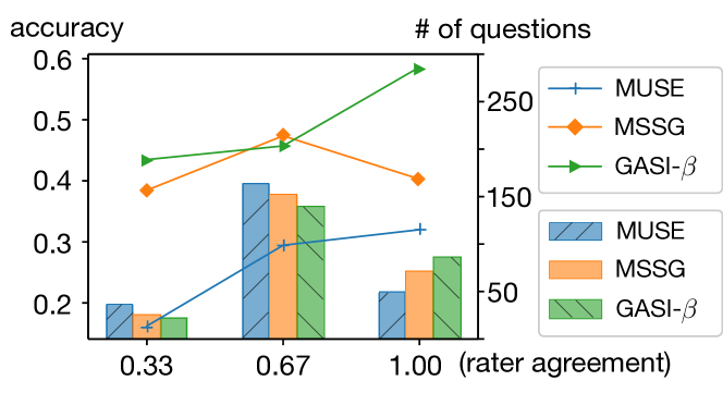
Figure 6: Higher inter-rater agreement correlates with higher human-model consistency.

Model	Accuracy(%)
unsupervised multi-prototype models
mssg-30k	54.00
muse_Boltzmann	52.14
gasi-$\beta$	55.27
semi-supervised with lexical resources
DeConf	58.55
sw2v	54.56

Table 8: Sense selection on Word in Context (wic) dataset.

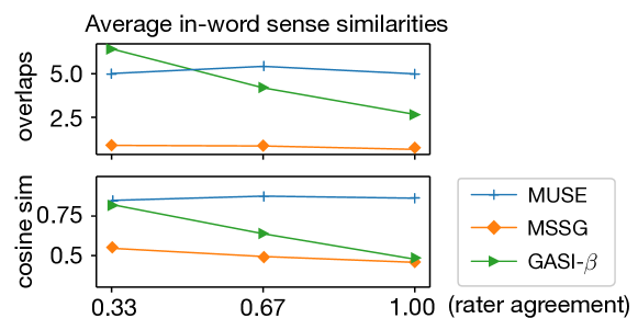
Figure 7: Overall, human agree more with each other when the senses are more distinct (less word overlaps and smaller cosine similarities)

References

- Athiwaratkun et al. (2018) Ben Athiwaratkun, Andrew Wilson, and Anima Anandkumar. 2018. Probabilistic fasttext for multi-sense word embeddings. In Proceedings of Empirical Methods in Natural Language Processing.
- Bartunov et al. (2016) Sergey Bartunov, Dmitry Kondrashkin, Anton Osokin, and Dmitry Vetrov. 2016. Breaking sticks and ambiguities with adaptive skip-gram. In Proceedings of Artificial Intelligence and Statistics.
- Brody and Lapata (2009) Samuel Brody and Mirella Lapata. 2009. Bayesian word sense induction. In Proceedings of the European Chapter of the Association for Computational Linguistics.
- Bruni et al. (2014) Elia Bruni, Nam-Khanh Tran, and Marco Baroni. 2014. Multimodal distributional semantics. Journal of Artificial Intelligence Research, 49.
- Camacho-Collados and Pilehvar (2018) José Camacho-Collados and Mohammad Taher Pilehvar. 2018. From word to sense embeddings: A survey on vector representations of meaning. CoRR, abs/1805.04032.
- Chang (2019) Henry Chang. 2019. Visualizing ELMo contextual vectors.
- Chang et al. (2009) Jonathan Chang, Jordan Boyd-Graber, Chong Wang, Sean Gerrish, and David M. Blei. 2009. Reading tea leaves: How humans interpret topic models. In Proceedings of Advances in Neural Information Processing Systems.
- Chen et al. (2015) Tao Chen, Ruifeng Xu, Yulan He, and Xuan Wang. 2015. Improving distributed representation of word sense via WordNet gloss composition and context clustering. In Proceedings of the Association for Computational Linguistics, pages 15–20. Association for Computational Linguistics.
- Chen et al. (2014) Xinxiong Chen, Zhiyuan Liu, and Maosong Sun. 2014. A unified model for word sense representation and disambiguation. In Proceedings of Empirical Methods in Natural Language Processing. Citeseer.
- Devlin et al. (2019) Jacob Devlin, Ming-Wei Chang, Kenton Lee, and Kristina Toutanova. 2019. BERT: Pre-training of deep bidirectional transformers for language understanding. In Conference of the North American Chapter of the Association for Computational Linguistics.
- Doshi-Velez and Kim (2017) Finale Doshi-Velez and Been Kim. 2017. Towards a rigorous science of interpretable machine learning. arXiv.
- Erk et al. (2009) Katrin Erk, Diana McCarthy, and Nicholas Gaylord. 2009. Investigations on word senses and word usages. In Proceedings of the Association for Computational Linguistics.
- Erk et al. (2013) Katrin Erk, Diana McCarthy, and Nicholas Gaylord. 2013. Measuring word meaning in context. Computational Linguistics, 39(3):511–554.
- Ettinger et al. (2016) Allyson Ettinger, Philip Resnik, and Marine Carpuat. 2016. Retrofitting sense-specific word vectors using parallel text. In Conference of the North American Chapter of the Association for Computational Linguistics.
- Feng and Boyd-Graber (2019) Shi Feng and Jordan Boyd-Graber. 2019. What ai can do for me: Evaluating machine learning interpretations in cooperative play. In International Conference on Intelligent User Interfaces.
- Figure Eight (2018) Figure Eight. 2018. How to calculate a confidence score. Https://success.figure-eight.com/hc/en-us/articles/201855939-How-to-Calculate-a-Confidence-Score.
- Finkelstein et al. (2002) Lev Finkelstein, Evgeniy Gabrilovich, Yossi Matias, Ehud Rivlin, Zach Solan, Gadi Wolfman, and Eytan Ruppin. 2002. Placing search in context: The concept revisited. ACM Transactions on Information Systems, 20(1).
- Gale et al. (1992) William A. Gale, Kenneth W. Church, and David Yarowsky. 1992. One sense per discourse. In Proceedings of the workshop on Speech and Natural Language.
- Goldberg and Levy (2014) Yoav Goldberg and Omer Levy. 2014. word2vec explained: Deriving mikolov et al.’s negative-sampling word-embedding method. arXiv preprint arXiv:1402.3722.
- Gumbel and Lieblein (1954) Emil Julius Gumbel and Julius Lieblein. 1954. Statistical theory of extreme values and some practical applications: a series of lectures. Technical report, US Government Printing Office Washington.
- Guo et al. (2014) Jiang Guo, Wanxiang Che, Haifeng Wang, and Ting Liu. 2014. Learning sense-specific word embeddings by exploiting bilingual resources. In Proceedings of International Conference on Computational Linguistics.
- Halawi et al. (2012) Guy Halawi, Gideon Dror, Evgeniy Gabrilovich, and Yehuda Koren. 2012. Large-scale learning of word relatedness with constraints. In Knowledge Discovery and Data Mining.
- Hamilton et al. (2016) William L. Hamilton, Jure Leskovec, and Dan Jurafsky. 2016. Diachronic word embeddings reveal statistical laws of semantic change. In Proceedings of the Association for Computational Linguistics.
- Hill et al. (2015) Felix Hill, Roi Reichart, and Anna Korhonen. 2015. Simlex-999: Evaluating semantic models with (genuine) similarity estimation. Computational Linguistics, 41(4).
- Huang et al. (2012) Eric H Huang, Richard Socher, Christopher D Manning, and Andrew Y Ng. 2012. Improving word representations via global context and multiple word prototypes. In Proceedings of the Association for Computational Linguistics.
- Iacobacci et al. (2015) Ignacio Iacobacci, Taher Mohammad Pilehvar, and Roberto Navigli. 2015. Sensembed: Learning sense embeddings for word and relational similarity. In Proceedings of the Association for Computational Linguistics, pages 95–105. Association for Computational Linguistics.
- Jang et al. (2016) Eric Jang, Shixiang Gu, and Ben Poole. 2016. Categorical reparameterization with gumbel-softmax. arXiv preprint arXiv:1611.01144.
- Jauhar et al. (2015) Sujay Kumar Jauhar, Chris Dyer, and Eduard Hovy. 2015. Ontologically grounded multi-sense representation learning for semantic vector space models. In Conference of the North American Chapter of the Association for Computational Linguistics.
- Jurgens and Klapaftis (2015) David Jurgens and Ioannis Klapaftis. 2015. Semeval-2013 task 13: Word sense induction for graded and non-graded senses. In Proceedings of the Workshop on Semantic Evaluation.
- Kawahara et al. (2014) Daisuke Kawahara, Daniel Peterson, Octavian Popescu, and Martha Palmer. 2014. Inducing example-based semantic frames from a massive amount of verb uses. In Proceedings of the European Chapter of the Association for Computational Linguistics.
- Labutov and Lipson (2013) Igor Labutov and Hod Lipson. 2013. Re-embedding words. In Proceedings of the Association for Computational Linguistics.
- Leacock et al. (1998) Claudia Leacock, George A. Miller, and Martin Chodorow. 1998. Using corpus statistics and wordnet relations for sense identification. Computational Linguistics, 24(1):147–165.
- Lee and Chen (2017) Guang-He Lee and Yun-Nung Chen. 2017. MUSE: Modularizing unsupervised sense embeddings. In Proceedings of Empirical Methods in Natural Language Processing.
- Li and Jurafsky (2015) Jiwei Li and Dan Jurafsky. 2015. Do multi-sense embeddings improve natural language understanding? arXiv preprint arXiv:1506.01070.
- Luong et al. (2013) Thang Luong, Richard Socher, and Christopher Manning. 2013. Better word representations with recursive neural networks for morphology. In Conference on Computational Natural Language Learning.
- Maaten and Hinton (2008) Laurens van der Maaten and Geoffrey Hinton. 2008. Visualizing data using t-sne. Journal of Machine Learning Research, 9(Nov).
- Maddison et al. (2016) Chris J Maddison, Andriy Mnih, and Yee Whye Teh. 2016. The concrete distribution: A continuous relaxation of discrete random variables. arXiv preprint arXiv:1611.00712.
- Mancini et al. (2017) Massimiliano Mancini, Jose Camacho-Collados, Ignacio Iacobacci, and Roberto Navigli. 2017. Embedding words and senses together via joint knowledge-enhanced training. In Conference on Computational Natural Language Learning.
- McCarthy et al. (2016) Diana McCarthy, Marianna Apidianaki, and Katrin Erk. 2016. Word sense clustering and clusterability. Computational Linguistics, 42(2):245–275.
- Mikolov et al. (2013a) Tomas Mikolov, Kai Chen, Greg Corrado, and Jeffrey Dean. 2013a. Efficient estimation of word representations in vector space. arXiv preprint arXiv:1301.3781.
- Mikolov et al. (2013b) Tomas Mikolov, Ilya Sutskever, Kai Chen, Greg S Corrado, and Jeff Dean. 2013b. Distributed representations of words and phrases and their compositionality. In Proceedings of Advances in Neural Information Processing Systems.
- Miller and Fellbaum (1998) George Miller and Christiane Fellbaum. 1998. Wordnet: An electronic lexical database. MIT Press Cambridge.
- Miller and Charles (1991) George A Miller and Walter G Charles. 1991. Contextual correlates of semantic similarity. Language and cognitive processes, 6.
- Miller et al. (1994) George A Miller, Martin Chodorow, Shari Landes, Claudia Leacock, and Robert G Thomas. 1994. Using a semantic concordance for sense identification. In Proceedings of the workshop on Human Language Technology.
- Miller et al. (2017) Tristan Miller, Christian Hempelmann, and Iryna Gurevych. 2017. SemEval-2017 task 7: Detection and interpretation of English puns. In Proceedings of the Workshop on Semantic Evaluation.
- Neelakantan et al. (2014) Arvind Neelakantan, Jeevan Shankar, Alexandre Passos, and Andrew McCallum. 2014. Efficient non-parametric estimation of multiple embeddings per word in vector space. In Proceedings of Empirical Methods in Natural Language Processing.
- Nguyen et al. (2017) Dai Quoc Nguyen, Dat Quoc Nguyen, Ashutosh Modi, Stefan Thater, and Manfred Pinkal. 2017. A mixture model for learning multi-sense word embeddings. In Proceedings of the Joint Conference on Lexical and Computational Semantics.
- Noraset et al. (2017) Thanapon Noraset, Chen Liang, Lawrence A Birnbaum, and Douglas C Downey. 2017. Definition modeling: Learning to define word embeddings in natural language. In Association for the Advancement of Artificial Intelligence.
- Orbanz and Teh (2010) P. Orbanz and Y. W. Teh. 2010. Bayesian Nonparametric Models. Springer.
- Pelevina et al. (2016) Maria Pelevina, Nikolay Arefiev, Chris Biemann, and Alexander Panchenko. 2016. Making sense of word embeddings. In Workshop on Representation Learning for NLP.
- Perone et al. (2018) Christian S Perone, Roberto Silveira, and Thomas S Paula. 2018. Evaluation of sentence embeddings in downstream and linguistic probing tasks. arXiv preprint arXiv:1806.06259.
- Peters et al. (2018) Matthew Peters, Mark Neumann, Mohit Iyyer, Matt Gardner, Christopher Clark, Kenton Lee, and Luke Zettlemoyer. 2018. Deep contextualized word representations. In Conference of the North American Chapter of the Association for Computational Linguistics.
- Pilehvar and Camacho-Collados (2018) Mohammad Taher Pilehvar and Jose Camacho-Collados. 2018. Wic: 10,000 example pairs for evaluating context-sensitive representations. arXiv preprint arXiv:1808.09121.
- Pilehvar and Collier (2016) Mohammad Taher Pilehvar and Nigel Collier. 2016. De-conflated semantic representations. In Proceedings of Empirical Methods in Natural Language Processing.
- Purandare and Pedersen (2004) Amruta Purandare and Ted Pedersen. 2004. Word sense discrimination by clustering contexts in vector and similarity spaces. In Conference on Computational Natural Language Learning.
- Qiu et al. (2016) Lin Qiu, Kewei Tu, and Yong Yu. 2016. Context-dependent sense embedding. In Proceedings of Empirical Methods in Natural Language Processing.
- Radinsky et al. (2011) Kira Radinsky, Eugene Agichtein, Evgeniy Gabrilovich, and Shaul Markovitch. 2011. A word at a time: computing word relatedness using temporal semantic analysis. In Proceedings of the World Wide Web Conference.
- Reisinger and Mooney (2010) Joseph Reisinger and Raymond J. Mooney. 2010. Multi-prototype vector-space models of word meaning. In Conference of the North American Chapter of the Association for Computational Linguistics.
- Rothe and Schütze (2017) Sascha Rothe and Hinrich Schütze. 2017. Autoextend: Combining word embeddings with semantic resources. Computational Linguistics, 43(3).
- Rubenstein and Goodenough (1965) Herbert Rubenstein and John B Goodenough. 1965. Contextual correlates of synonymy. Communications of the ACM, 8(10).
- Schnabel et al. (2015) Tobias Schnabel, Igor Labutov, David M. Mimno, and Thorsten Joachims. 2015. Evaluation methods for unsupervised word embeddings. In Proceedings of Empirical Methods in Natural Language Processing.
- Schütze (1998) Hinrich Schütze. 1998. Automatic word sense discrimination. Computational linguistics, 24(1).
- Shaoul C. (2010) Westbury C Shaoul C. 2010. The Westbury Lab Wikipedia Corpusa.
- Šuster et al. (2016) Simon Šuster, Ivan Titov, and Gertjan van Noord. 2016. Bilingual learning of multi-sense embeddings with discrete autoencoders. In Conference of the North American Chapter of the Association for Computational Linguistics.
- Tian et al. (2014) Fei Tian, Hanjun Dai, Jiang Bian, Bin Gao, Rui Zhang, Enhong Chen, and Tie-Yan Liu. 2014. A probabilistic model for learning multi-prototype word embeddings. In Proceedings of International Conference on Computational Linguistics.
- Wang et al. (2011) Chong Wang, John Paisley, and David M. Blei. 2011. Online variational inference for the hierarchical Dirichlet process. In Proceedings of Artificial Intelligence and Statistics.
- Wu and Giles (2015) Zhaohui Wu and C Giles. 2015. Sense-aaware semantic analysis: A multi-prototype word representation model using Wikipedia. In Association for the Advancement of Artificial Intelligence.
- Yang and Powers (2006) Dongqiang Yang and David Martin Powers. 2006. Verb similarity on the taxonomy of WordNet. Masaryk University.