MQGrad: Reinforcement Learning of Gradient Quantization in Parameter Server
Abstract
One of the most significant bottleneck in training large scale machine learning models on parameter server (PS) is the communication overhead, because it needs to frequently exchange the model gradients between the workers and servers during the training iterations. Gradient quantization has been proposed as an effective approach to reducing the communication volume. One key issue in gradient quantization is setting the number of bits for quantizing the gradients. Small number of bits can significantly reduce the communication overhead while hurts the gradient accuracies, and vise versa. An ideal quantization method would dynamically balance the communication overhead and model accuracy, through adjusting the number bits according to the knowledge learned from the immediate past training iterations. Existing methods, however, quantize the gradients either with fixed number of bits, or with predefined heuristic rules. In this paper we propose a novel adaptive quantization method within the framework of reinforcement learning. The method, referred to as MQGrad, formalizes the selection of quantization bits as actions in a Markov decision process (MDP) where the MDP states records the information collected from the past optimization iterations (e.g., the sequence of the loss function values). During the training iterations of a machine learning algorithm, MQGrad continuously updates the MDP state according to the changes of the loss function. Based on the information, MDP learns to select the optimal actions (number of bits) to quantize the gradients. Experimental results based on a benchmark dataset showed that MQGrad can accelerate the learning of a large scale deep neural network while keeping its prediction accuracies.
1 Introduction
With the rapid growth of the training data and the resulting machine learning model complexity, distributed optimization has become a popular solution for scaling up the machine learning problems. Parameters sever (PS) [?] is one of the most popularly adopted distributed computing framework tailored for large scale machine learning. PS splits the computers in a cluster into worker nodes and server nodes. The data and workload are distributed to worker nodes and the globally shared model parameters are maintained by the server nodes. During the training of machine learning models, the worker nodes process data and calculate the gradients while server nodes synchronize parameters and perform global updates. PS can scale up a number of machine learning algorithms such as LDA and logistic regression.
It has been observed that the communication overhead is one of the major bottleneck in PS[?; ?]. At each of the optimization iteration, after finishing the local computations, multiple worker nodes need to push the resulting gradients of the parameters to the corresponding server nodes for parameter updating, and then pull the updated parameters to local for next iteration computations. Since the optimization procedure needs to execute a large number of iterations, the communication volume between the worker nodes and server nodes is huge and time consuming. Thus, how to reduce the communication volume becomes a key problem for accelerating the training of machine learning algorithms on PS.
Gradient quantization has been proposed as one of the most effective approach to reduce the communication overhead in distributed systems [?; ?; ?]. It reduces the number of bits used to transmit each parameter through quantizing (compressing) the transmitted values. When applying gradient quantization in PS, how to determine the number of bits used to transit each parameter, aka the quantization bits, is a critical issue. On one hand, one may want to set a small quantization bits for significantly reducing the communication overhead. On the other hand, the quantization bits cannot be too small because heavily compressing the gradients inevitably makes the model inaccurate, which may slow down the decreasing of the loss or even make the optimization not converge. How to balance between the communication overhead and gradient accuracy is one of the key issues in gradient quantization.
Ideally, for choosing optimal quantization bits at each iteration, PS system would dynamically adjust the bits with the knowledge learned from the past optimization iterations (e.g., the decreasing rates of the loss function at the past a few iterations). Existing approaches, however, usually choose a fixed quantization bits before running the machine learning algorithm [?; ?]. In recent years methods are proposed in which the quantization bits can be dynamically adjusted with predefined heuristic rules. For example, ? proposes to adjust the quantization bits according to the norm of gradient vector. The experience from the past optimization iterations is not fully utilized.
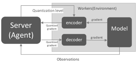
In this paper, we aim at developing a new method that can learn to adjust the quantization bits, on the basis of the information collected from the past optimization iterations. Inspired by the success of learning to learn [?] and reinforcement learning, we propose to use the Markov decision process (MDP) to learn the quantization bits in PS, referred to as MQGrad. The agent-environment interaction framework of MQGrad is shown in Figure 1. MQGrad formalizes the adjustment of the quantization bits as actions in an MDP. At each iteration of training the machine learning algorithm, the MQGrad agent repeatedly monitors the values of the machine learning loss function for updating its state and calculating the rewards. Then, it chooses the best action (quantization bits) and sends it to the workers for quantizing the gradients at the current iteration. The reinforcement algorithm of SARSA [?] is utilized here for determining the quantization bits and updating the parameters of the MDP model.
MQGrad offers several advantages: ease in implementation, ability of balancing the communication overhead and model accuracy automatically, and effectively accelerating the large scale machine learning algorithms.
Experimental results indicate that MQGrad can outperform the baseline quantization methods including the fixed quantization methods and the adaptive quantization, in terms of accelerating a deep learning algorithm trained on CIFAR-10 dataset.
2 Related work
A lot of research efforts have been spent for accelerating the distributed (machine learning) systems through reducing the communication cost of the system.
One direct approach to minimize communication overhead is just to reduce the number of parameters need to be exchanged, e.g. by having fewer parameters in the first place by sparsifying them. In the early works[?; ?; ?; ?], network pruning has been proved as a valid way to reduce the complexity of the network. Recently, ? pruned state-of-the-art CNN models with no loss of accuracy and ? prunes the network’s connections by removing all connections with weights below a threshold to reduce the parameters.
Another way to reduce the communication overhead is using less bits to represent the parameters or gradients, called parameter or gradient quantization. For example, ? uses 1 bit to quantize the gradients which greatly reduce the communication overhead while it needs the quantization error to be carried forward across mini-batches. ? proposed quantized SGD(QSGD) which is a family of compression schemes with convergence guarantees and good practical performance. ? used similar stochastic quantization like QSGD but focused on using three possible values to represent each value of gradient. ? reduced the communication overhead by nearly an order of magnitude through adaptively choosing the bits to quantize the weights according to gradient’s mean square error. The method is based on the simple hypothesis: when the gradient’s norm is large, more bits are needed to represent the gradient because relatively small perturbations can result in relatively large changes in the error.
All existing parameter quantization methods cannot utilize the knowledge from the optimization history. In this paper, we propose to learn to set the quantization bits, on the basis of the data collected from the past training iterations. The idea is similar to that of “learning to learn” [?] which automatically learns the updating rule of optimization in machine learning. A number of learning to learn algorithms has been proposed in the past a few years and reinforcement learning is also used for the task. For example, reinforcement learning algorithms are used for tuning the learning rate [?; ?; ?], for optimizing device placement for Tensorflow computational graphs[?], and for generating network architecture to maximize the expected accuracy of the validate set [?]. In this paper, we make use of the reinforcement learning model of MDP to learn the quantization bits for compressing the gradients.
3 Our Approach: MQGrad
In this section, we describe the proposed MQGrad model for reducing the communication overhead in PS.
3.1 Background: machine learning with PS
The goal of many machine learning algorithms can be formalized as minimizing a “loss function” which captures the properties of the learned model, e.g., the error in terms of the training data and the complexity of the learned model. In general, there is no closed-form solution for the optimization problem. Instead, the training starts from an initial model. It iteratively refines the model by processing the training data and stops when a (near) optimal solution is found or the model is considered to be converged.
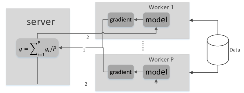
In a distributed computing environment, we usually split the training data in multiple workers and send each worker the same parameters at first. Each worker computes gradient of the loss function with respect to parameters based on the training data it has and then sends the gradient to the server. Server collects gradients from all workers, averages it and then sends the gradient to all workers for updating the parameters. Figure 2 shows the process.
Usually a PS system spends a lot of time to communicate the gradients between sever nodes and worker nodes, as the number of parameters is large and they need to be transfered at each of the training iteration. Gradient quantization has been widely used to reduce the communication overhead and accelerate the training process. In the following sections, we describe our proposed MQGrad model which learns to adjust the quantization bits with reinforcement learning.
3.2 MQGrad system architecture
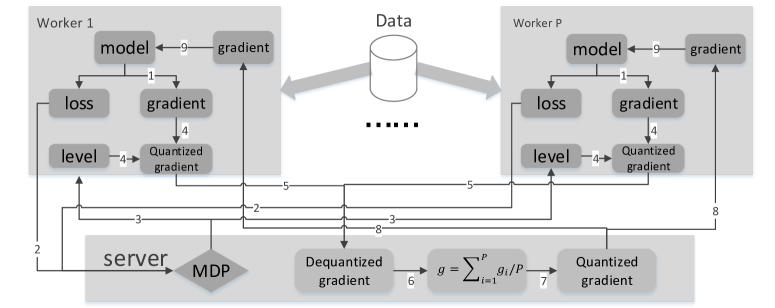
We extend the PS architecture shown in Figure 2 with an MDP module on the sever side and gradient quantize/de-quantize modules on all of the nodes, achieving the MQGrad system shown in Figure 3 and the functions executed on the scheduler, workers, and servers are shown in Algorithm 1.
Suppose that a large scale machine learning model is being trained on the PS. After distributing the training data and the model parameters (necessary working set) to each worker node, the training algorithm executes an iterative optimization of its loss function. At each iteration , given the current model parameters, the training algorithm calculates the local gradients at each worker node. At the same time, each worker also calculates the local value of the loss function based on the local data (step 1 in Fig. 3, line 28 in Alg. 1). The local values at all of the workers are collected by the sever MDP module (step 2 in Fig. 3, line 38 of Alg. 1). After that, the MDP module at server restores the overall global loss, updates its state, calculates the reward, determines the action (the quantization bits), and finally broadcasts the number to all worker nodes (step 3 in Fig. 3, line 39-47 in Alg. 1). Given the quantization bits, the worker nodes quantize111MQGrad uses the Quantize (Encode) and De-quantize (Decode) functions in https://www.tensorflow.org/performance/quantization. their local gradients (step 4 in Fig. 3, line 30 in Alg. 1) and send the quantized local gradients to the parameter server (step 5 in Fig. 3, line 31 in Alg. 1). The server nodes de-quantize and summarize all of the received local gradients to a global gradient for updating the model parameters (step 6 and 7 in Fig. 3, line 51-52 in Alg. 1). Then the server broadcasts the quantized global gradient (step 8 in Fig. 3, line 53 in Alg. 1) and the workers receive it, de-quantize the gradient, and update the local model parameters (step 9 in Fig. 3, line 32-33 in Alg. 1).
Receiving the signal that the model parameters have been updated, the machine learning training algorithm moves to iteration and re-estimates the local gradients and local losses. The process repeats until converge or the number of iterations reaches a predefined maximum number.
3.3 Learning for gradient quantization with MDP
The key component in MQGrad is the MDP module which determines the quantization bits. The configuration of the MDP is as follows:
Time step : is the discrete time step of the MDP. To avoid adjusting the quantization bits too frequently, which may result in an unstable training process, the MDP model in MQGrad is configured to update the quantization bits every training iterations. That is, the server will broadcast the identical quantization bits used in the last iteration to worker nodes (step 3 in Figure 3) if , where is the iteration number of the machine learning training algorithm. During these iterations, the MDP module only collects the losses for constructing its state. The MDP module will be activated to update the quantization bits when . Thus the MDP time step . In this paper, we empirically set , which means the MDP time step is 5 times slower than the number of training iterations. Note that both and start from 0.
States : The MDP state at time step is denoted as , where is the most confident quantization bits at time step , predicted by the function; is calculated as follows: at time step , the MDP receives consequent global losses, denoted as , where is the global loss calculated based on the local losses received at the training iteration . The global losses reflect the goodness of the quantization bits used at the last iterations. These values, however, may vary to a large extent. To make the statistics of these losses stable, following the practices in [?], MQGrad makes use of the moving average technique to smooth these losses:
| (1) |
where is the parameter. Thus is a sequence of values: .
Actions : MQGrad has two actions at each time step: , where keeps the current quantization bits and increases the quantization bits by one. Thus given and the chosen action , the quantization bits for the immediate next training iterations is , where is the quantization bits in state . Note that MQGrad does not decrease the quantization bits. The configuration is based on the observation that with the machine learning training iteration goes on, more accurate gradients are needed to update the model parameters because the parameters are closer to the optimal solution. Experimental results also showed that the configuration can achieve better results.
function: The function predicts the value of taking action at the state s following policy . Following the practice in DQN [?], MQGRad configures the function as a neural network (parameterized by v). The input to the neural network is the state and the outputs are the confidence values for the available actions. The parameter v will be updated during the MDP iterations with SARSA algorithm [?].
Policy : defines the probability of selecting an action at state s. We define the policy with the -greedy criteria for balancing the exploration and exploitation. Specifically, at the MDP time step , given the state , the probability of selecting an action is denoted as and defined as:
Reward : MQGrad calculates the reward on the basis of the consequent losses collected from the last training iterations and the total time cost for executing the iterations. Intuitively, small decrease in loss with high time cost makes the reward small, and vise versa. Specifically, suppose that the moving averaged losses are and the time cost for executing the last training iterations is (in milliseconds). MQGrad solves the following linear regression problem for getting the decreasing rate with respect to iteration :
where is the bias. The reward is calculated as:
| (2) |
where is a scaling parameter.
Transition : The transition function defines the transition of the MDP state. The output of also consists of two parts: . These two components are calculated as:
| (3) |
After selecting on the basis of , the server broadcasts the quantization bits (where is the quantization bits in ) to all of the worker nodes. MQGrad then monitors and collects the losses of the immediate training iterations and constructs a sequence of moving averaged losses , on the basis of Equation (1). As for , if , MQGrad keeps . Otherwise, MQGrad increases the quantization bits in state by 1.
During the running of the MDP, the SARSA algorithm is used for determining the quantization bits and learning the parameters in function, as shown in Algorithm 2. The running of the MDP in MQGrad can be described as follows: at each MDP time step , the agent(server) receives the state (line 1 of Alg. 2) and the reward (line 2 of Alg. 2). Then an action is selected on the basis of the policy (line 3 of Alg. 2). After that, the system updates the parameter v of the network (line 4 of Alg. 2). Finally the number of bits is returned for conducting the gradient quantization (line 5 of Alg. 2).
The source code of MQGrad can be found in the Github http://hide_due_to_annonymous_review.
4 Experiments
4.1 Experimental settings
To test the performances of the proposed MQGrad system, experiments were conducted on two PS clusters. One consists of 12 nodes and the other consists of 18 nodes. Each nodes in the clusters contains 4 cores each of which has a frequency of 2.3GHz and these nodes were connected by a network with 10MB/s bandwidth.
The experiments were conducted on the basis of the CIFAR-10 [?] dataset. The machine learning algorithm tested is a 5-layer neural network: the first two are convolutional layers with each layers’ parameter’s shape being and . Local response normalization after max-pooling is used [?]. The third and fourth layers are fully connected layers with shapes and , respectively. The last softmax layer is also a fully connected layer with shape . Cross entropy loss with norm of the third layer and fourth layer’s parameters are used as the loss function. During the training, the batch size is set to 32 and the learning rate is set to 0.2. Considering the third and fourth layers have about 99.2% of the network parameters, gradient quantization is applied to these two layers. Other parameters are communicated without any compression.
The range of quantization bits is set to 2 to 8 bits (7 levels). The function has three layers: the first layer contains 5 nodes, representing the 5 average smoothed values in state . The second layer contains 10 nodes with ReLU activation. The third layer is a linear layer which has 7 nodes, each corresponds to a quantization bits.
MQGrad has some hyper parameters. The variables in SARSA and . The moving average parameter and the scaling variable .
We compared MQGrad with several state-of-the-arts baselines in gradient quantization, including the adaptive quantization method [?] (denoted as “Adaptive” in the paper) and the fixed quantization methods. For the fixed bit quantization methods, the numbers of quantization bits were set to 2, 4, and 8 and denoted as “Fix (2-bit)”, “Fix (4-bit)”, and “Fix (8-bit)”, respectively.
4.2 Experimental results
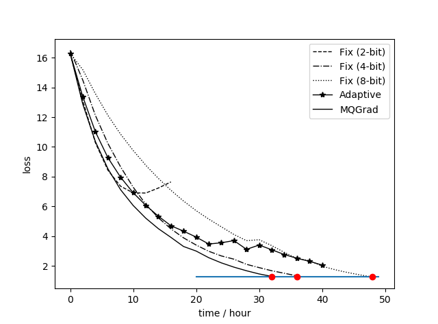
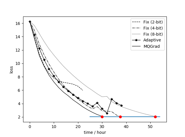
Figure 4 and Figure 5 show the training curves of “MQGrad” as well as the baselines in terms of the neural network loss being optimized, on the 12-node PS cluster and the 18-node PS cluster, respectively. The x-axises indicate the training time (in terms of hours). From the results, we can see that “MQGrad” outperformed all the baseline methods (used less training time to reach smaller loss) on both of these two clusters. For example, compared with the best baseline “Fix (4-bit)”, “MQGRad” used less 7.5 hours to reach the same loss on the 18-node cluster. The results indicate the effectiveness of using reinforcement learning for gradient quantization.
From the results, we can also see that the training curve “Fix (2-bit)” decreased the loss function very fast during the first ten hours. However, it did not converge in the remaining training time. The phenomenon indicated that at the early stage of the training low quantization bits helped to minimize the loss function fast. However, with the training goes on, high accurate gradients were necessary and the low quantization bits hurt the convergence. On the other hand, the training curve of “Fix (8-bit)”, which used more bits for quantizing the gradients during the training, steadily decreased during all of the training time. However, the decreasing speed was slow because a lot of time was wasted for transiting the gradients. Thus, “Fix (8-bit)” needed longer time to converge. “MQGrad” made a good trade-off: it used low quantization bits at the early training stages for saving the communication volume, and gradually increased the quantization bits for increasing the gradient accuracies. The method of “Adaptive” can also decrease the communication volume at the early training stages. However, the predefined heuristics in “Adaptive” cannot make good decisions to guarantee the gradient accuracy at the later training phases.
We also tested the model accuracies for these methods. Table 1 and Table 2 show the results on the 12-node cluster and 18-node cluster, respectively. “N/A” indicates the result is not available because the model has converged at the time. From the results we can see that the accuracies of MQGrad are higher than the baselines when trained with the same time, indicating the lower loss leads to higher performances. The final converged performances of MQGrad are comparable to “Adaptive” and “Fix (8-bit)”, indicating MQGrad can accelerate the training process while keeping model accuracies.
| 5 hours | 15 hours | 30 hours | 40 hours | |
|---|---|---|---|---|
| Fix (2-bit) | 50.8 | 55.9 | N/A | N/A |
| Fix (4-bit) | 41.9 | 57.5 | 66.7 | N/A |
| Fix (8-bit) | 35.7 | 55.6 | 60.8 | 68.1 |
| Adaptive | 49.4 | 60.1 | 65.3 | N/A |
| MQGrad | 54.7 | 65.6 | 67.7 | N/A |
| 5 hours | 15 hours | 30 hours | 40 hours | |
|---|---|---|---|---|
| Fix (2-bit) | 51.5 | 58.5 | N/A | N/A |
| Fix (4-bit) | 45.4 | 57.9 | 68.4 | N/A |
| Fix (8-bit) | 42.1 | 58.2 | 65.9 | 68.2 |
| Adaptive | 43.6 | 57.3 | 63.4 | N/A |
| MQGrad | 51.5 | 62.0 | 68.2 | N/A |
|
|
|
Adaptive | MQGrad | |||||||
|---|---|---|---|---|---|---|---|---|---|---|---|
| 12-node cluster | 13.3 | 8.0 | 4.44 | 8.13 | 7.41 | ||||||
| 18-node cluster | 11.4 | 7.27 | 4.21 | 5.84 | 4.11 |
Note that the execution of the quantization/de-quantization (and the MDP) modules in the baselines and MQGrad needs some additional time. We conducted experiments to show the fraction of these additional time among the whole training time. From the results shown in Table 3, we can see that on the 12-node and the 18-node clusters, MQGrad respectively need 7.41% and 4.11% of the time for running the quantization, de-quantization, and the MDP modules. For other baseline methods, most of the fractions are less than 10%. The results indicate that 1) the additional time costs caused by MDP module in MQGrad is negligible; 2) the time cost for quantizing/de-quantizing gradients is not high, making all of these methods can accelerate the overall training iterations.
5 Conclusion
In the paper we propose a novel gradient quantization method called MQGrad, for accelerating the distributed machine learning algorithms on parameter server. MQGrad learns to determine the number of bits for gradient quantization with the information collected from the past optimization iterations. MDP is used to formalize the process and the on-policy learning algorithm SARSA is used to learn the quantization bits and update the MDP parameters. Experimental results on a benchmark dataset showed that MQGrad outperformed the state-of-the-arts gradient quantization methods, in terms of accelerate the speeds of learning large scale machine learning models. Analysis showed that MQGrad accelerated the learning speeds through lowering the communication volume at the early stage of training and gradually improving the gradient accuracies with the training went on.
References
- [Alistarh et al., 2016] Dan Alistarh, Jerry Li, Ryota Tomioka, and Milan Vojnovic. Qsgd: Randomized quantization for communication-optimal stochastic gradient descent. arXiv preprint arXiv:1610.02132, 2016.
- [Andrychowicz et al., 2016] Marcin Andrychowicz, Misha Denil, Sergio Gomez, Matthew W Hoffman, David Pfau, Tom Schaul, and Nando de Freitas. Learning to learn by gradient descent by gradient descent. In Advances in Neural Information Processing Systems, pages 3981–3989, 2016.
- [Daniel et al., 2016] Christian Daniel, Jonathan Taylor, and Sebastian Nowozin. Learning step size controllers for robust neural network training. In AAAI, pages 1519–1525, 2016.
- [Dean et al., 2012] Jeffrey Dean, Greg Corrado, Rajat Monga, Kai Chen, Matthieu Devin, Mark Mao, Andrew Senior, Paul Tucker, Ke Yang, Quoc V Le, et al. Large scale distributed deep networks. In Advances in neural information processing systems, pages 1223–1231, 2012.
- [Fu et al., 2016] Jie Fu, Zichuan Lin, Miao Liu, Nicholas Leonard, Jiashi Feng, and Tat-Seng Chua. Deep q-networks for accelerating the training of deep neural networks. arXiv preprint arXiv:1606.01467, 2016.
- [Han et al., 2015] Song Han, Huizi Mao, and William J Dally. Deep compression: Compressing deep neural networks with pruning, trained quantization and huffman coding. arXiv preprint arXiv:1510.00149, 2015.
- [Han et al., 2016] Song Han, Xingyu Liu, Huizi Mao, Jing Pu, Ardavan Pedram, Mark A Horowitz, and William J Dally. Eie: efficient inference engine on compressed deep neural network. In Computer Architecture (ISCA), 2016 ACM/IEEE 43rd Annual International Symposium on, pages 243–254. IEEE, 2016.
- [Hanson and Pratt, 1989] Stephen José Hanson and Lorien Y Pratt. Comparing biases for minimal network construction with back-propagation. In Advances in neural information processing systems, pages 177–185, 1989.
- [Hassibi and Stork, 1993] Babak Hassibi and David G Stork. Second order derivatives for network pruning: Optimal brain surgeon. In Advances in neural information processing systems, pages 164–171, 1993.
- [Ho et al., 2013] Qirong Ho, James Cipar, Henggang Cui, Seunghak Lee, Jin Kyu Kim, Phillip B Gibbons, Garth A Gibson, Greg Ganger, and Eric P Xing. More effective distributed ml via a stale synchronous parallel parameter server. In Advances in neural information processing systems, pages 1223–1231, 2013.
- [Krizhevsky and Hinton, 2009] Alex Krizhevsky and Geoffrey Hinton. Learning multiple layers of features from tiny images. 2009.
- [Krizhevsky et al., 2012] Alex Krizhevsky, Ilya Sutskever, and Geoffrey E Hinton. Imagenet classification with deep convolutional neural networks. In Advances in neural information processing systems, pages 1097–1105, 2012.
- [LeCun et al., 1990] Yann LeCun, John S Denker, and Sara A Solla. Optimal brain damage. In Advances in neural information processing systems, pages 598–605, 1990.
- [Li et al., 2014] Mu Li, David G Andersen, Jun Woo Park, Alexander J Smola, Amr Ahmed, Vanja Josifovski, James Long, Eugene J Shekita, and Bor-Yiing Su. Scaling distributed machine learning with the parameter server. In OSDI, volume 1, page 3, 2014.
- [Mirhoseini et al., 2017] Azalia Mirhoseini, Hieu Pham, Quoc V Le, Benoit Steiner, Rasmus Larsen, Yuefeng Zhou, Naveen Kumar, Mohammad Norouzi, Samy Bengio, and Jeff Dean. Device placement optimization with reinforcement learning. arXiv preprint arXiv:1706.04972, 2017.
- [Mnih et al., 2013] Volodymyr Mnih, Koray Kavukcuoglu, David Silver, Alex Graves, Ioannis Antonoglou, Daan Wierstra, and Martin Riedmiller. Playing atari with deep reinforcement learning. arXiv preprint arXiv:1312.5602, 2013.
- [Øland and Raj, 2015] Anders Øland and Bhiksha Raj. Reducing communication overhead in distributed learning by an order of magnitude (almost). In Acoustics, Speech and Signal Processing (ICASSP), 2015 IEEE International Conference on, pages 2219–2223. IEEE, 2015.
- [Seide et al., 2014] Frank Seide, Hao Fu, Jasha Droppo, Gang Li, and Dong Yu. it stochastic gradient descent a1-bnd its application to data-parallel distributed training of speech dnns. In Fifteenth Annual Conference of the International Speech Communication Association, 2014.
- [Ström, 1997] Nikko Ström. Phoneme probability estimation with dynamic sparsely connected artificial neural networks. The Free Speech Journal, 5:1–41, 1997.
- [Sutton and Barto, 1998] Richard S Sutton and Andrew G Barto. Reinforcement learning: An introduction, volume 1. MIT press Cambridge, 1998.
- [Wen et al., 2017] Wei Wen, Cong Xu, Feng Yan, Chunpeng Wu, Yandan Wang, Yiran Chen, and Hai Li. Terngrad: Ternary gradients to reduce communication in distributed deep learning. arXiv preprint arXiv:1705.07878, 2017.
- [Xu et al., 2017] Chang Xu, Tao Qin, Gang Wang, and Tie-Yan Liu. Reinforcement learning for learning rate control. arXiv preprint arXiv:1705.11159, 2017.
- [Zoph and Le, 2016] Barret Zoph and Quoc V Le. Neural architecture search with reinforcement learning. arXiv preprint arXiv:1611.01578, 2016.