The Advantage of Foraging Myopically

Abstract

We study the dynamics of a myopic forager that randomly wanders on a lattice in which each site contains one unit of food. Upon encountering a food-containing site, the forager eats all the food at this site with probability $p<1$; otherwise, the food is left undisturbed. When the forager eats, it can wander $\mathcal{S}$ additional steps without food before starving to death. When the forager does not eat, either by not detecting food on a full site or by encountering an empty site, the forager goes hungry and comes one time unit closer to starvation. As the forager wanders, a multiply connected spatial region where food has been consumed—a desert—is created. The forager lifetime depends non-monotonically on its degree of myopia $p$, and at the optimal myopia $p=p^{*}(\mathcal{S})$, the forager lives much longer than a normal forager that always eats when it encounters food. This optimal lifetime grows as $\mathcal{S}^{2}/\ln\mathcal{S}$ in one dimension and faster than a power law in $\mathcal{S}$ in two and higher dimensions.

1 Introduction and Model

In this work, we extend of the starving random walk model of foraging [1, 2] to the situation where the forager is myopic. Whenever such a forager comes to a site that contains food, all the food at this site is eaten with probability $p$, while the food is left undisturbed with probability $1-p$. In the limiting case of $p=1$, the forager always consumes food when it is encountered. This rule corresponds to the original starving random walk, which here we term the normal forager. We want to understand the role of myopia—quantified by $p$—on the foraging dynamics and on the geometry of the “desert”, the region where food has been consumed. Our main results are: (a) the forager lifetime depends non-monotonically on $p$, (b) at an optimal value of $p$, the forager lifetime is much longer than that of a normal forager (with $p=1$), and (c) the average geometry of the desert has a simple character, even though the desert geometry for each individual trajectory is complex (Fig. 1).

Foraging is a fundamental biological process that has been extensively investigated and documented in the ecology literature (see e.g., Refs. [3, 4, 5, 6, 7, 8]). In classic theories of foraging, a typical assumption is that the forager has complete knowledge of its environment and makes rational decisions about when to continue exploiting a local resource and when to explore a new search domain. The starving random walk model represents a complementary perspective in which the forager has no knowledge of its environment and uses naive decision rules to search for resources.

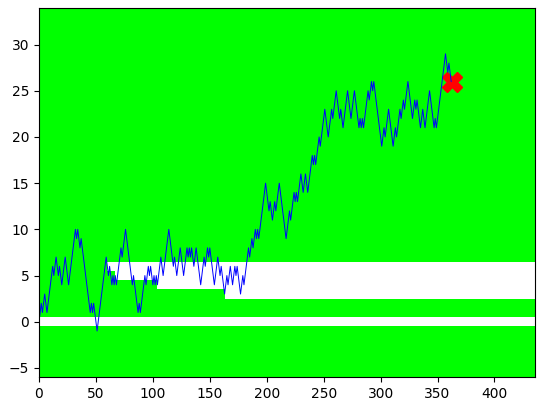
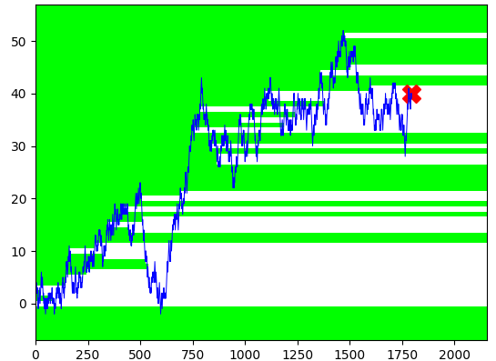
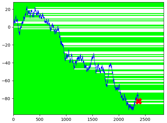
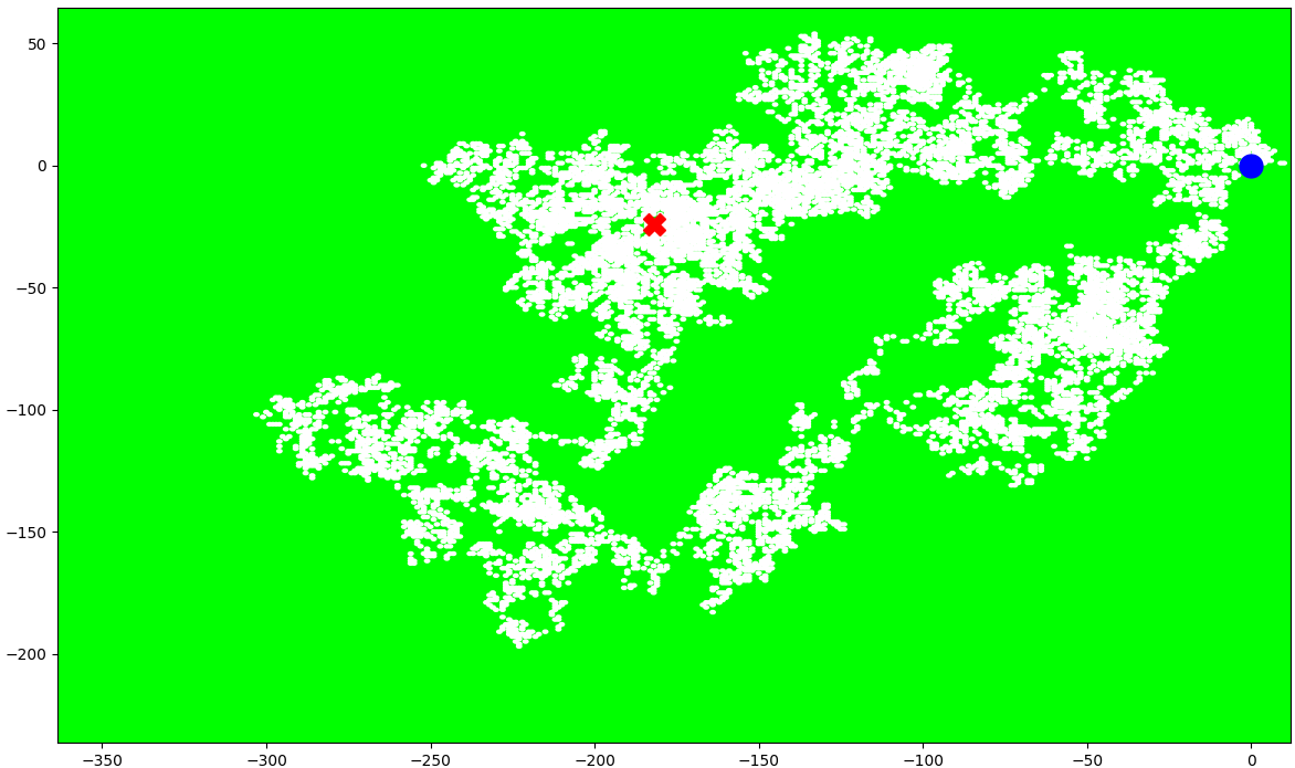
Figure 1: Typical space-time trajectories of a myopic forager with $\mathcal{S}=200$ and $p=p^{*}\approx 0.035$ in dimension $d=1$ (a)–(c) and $\mathcal{S}=100$ and $p=0.2$ in $d=2$ (d). Green shaded area represents food and white space denotes desert. In $d=2$, the starting location of the forager is indicated by the blue dot.

In the starving random walk model, a forager performs a random walk on an infinite lattice, independent of the presence of absence of resources in its local neighborhood [1, 2]. When the forager lands on a food-containing site, all the food at this site is consumed. Upon eating, a forager is fully satiated and can hop $\mathcal{S}$ additional steps without again eating before it starves. Upon landing on an empty site, the forager goes hungry and comes one time unit closer to starvation. The forager starves when it last ate $\mathcal{S}$ steps in the past. We may therefore view $\mathcal{S}$ as the metabolic storage capacity of the forager. Because there is no resource replenishment, the forager is doomed to ultimately starve and the basic question is: when does the forager starve?

This starving random walk model was recently extended to incorporate, in a minimalist way, various aspects of real foraging. As one example [9, 10], a forager was endowed with the attribute of greed, in which it moves preferentially towards food if the forager has a choice between hopping to an empty site or a food-containing site in its local neighborhood. It was found that there exists an optimal greediness that maximizes the forager lifetime in two dimensions, and an optimal value of negative greed (where the forager tends to avoid food in its local neighborhood) that maximizes the lifetime in one dimension. The starving random walk was also extended to incorporate frugality, in which the forager eats only if it is nutritionally depleted beyond a specified level when it lands on a food-containing site [11]. It was found that the forager lifetime is maximized at an optimal frugality level.

The issues that we address in this work are: How does the myopia of a forager affect its lifetime and the geometry of the desert that is created? An important consequence of myopia is that the desert is no longer simply connected (Fig. 1). In dimension $d=1$, the desert consists of multiple empty segments that are interspersed with oases—food-containing segments. As the forager wanders, it may nucleate a new desert segment when it eats food within a previously undepleted region; conversely, the forager may consume all the food in an oasis thereby joining disconnected desert segments. The connectedness of the desert in the original starving random walk model was a crucial feature that allowed for an asymptotic solution of the lifetime in $d=1$ [1, 2]. The multiple connectedness of the desert (Figs. 1(a)–(c)) for the myopic forager introduces a new layer of complexity to this challenging non-Markovian process; the problem in $d>1$ is geometrically even more complex (Fig. 1(d)).

In the next section, we first present a heuristic argument that accounts for the behavior of the forager lifetime for small $p$ in any spatial dimension. We also argue that the lifetime must depend non-monotonically on the myopia parameter $p$, at least in low spatial dimensions. In the following two sections, we present simulation results for the optimal myopia value and for the forager lifetime at the optimal myopia in spatial dimensions $d=1$, 2 and 3. We find that this maximal forager lifetime grows as $\mathcal{S}^{2}/\ln\mathcal{S}$ $d=1$, and grows faster than any power law in $\mathcal{S}$ for $d\geq 2$. In both $d=1$ and $d=2$, the average density profile of the desert decays exponentially in the distance from the starting point of the forager.

2 Heuristics

Because of the geometrical complication that the myopic forager carves out a multiply-connected desert, the approach used to analyze the dynamics of the normal forager in a single-segment desert, is not applicable here [1, 2]. However, we can understand the behavior of the lifetime when $p$ is within a suitable range. The extreme case of $p\ll\mathcal{S}^{-1}$ is uninteresting because the forager typically does not eat before it starves, so that its lifetime equals $\mathcal{S}$. Thus we examine the case where $p$ is small, but with $p>\mathcal{S}^{-1}$, so that the forager typically eats multiple times before it starves.

Figure 2: State space of the myopic forager in the limit of small $p$.

In this range of $p\gtrsim\mathcal{S}^{-1}$, but with $p\ll 1$, it is unlikely that the forager will revisit a site where food was previously consumed. Thus we assume that the forager always lands on a full site and check the validity of this assumption at the end of the calculation. If there is no depletion, there are only two outcomes after the forager takes a single step: it either eats with probability $p$, or does not eat with probability $1-p$. The state space for this process is depicted in Fig. 2; this same state-space geometry also arises in models of kinetic proofreading [12, 13, 14] and in the starving random walk in the mean-field limit [2]. The forager starts in the fully satiated state, corresponding to the right edge of the interval of length $\mathcal{S}$ in the figure. When the forager does not eat, it comes one time unit closer to starvation and thus hops one step to the left in state space. When the forager eats, it is fully satiated and hops all the way to the right edge of the interval. Starvation corresponds to the forager reaching site 0. The forager lifetime $\mathcal{T}$ is just the mean time for the particle in this state space to first reach site 0 when starting from site $\mathcal{S}$ (Fig. 2). This time can be determined by the formalism of Ref. [15] and was previously computed in Ref. [2] to be:

$$\mathcal{T}=\frac{1}{p}\big{[}(1-p)^{-\mathcal{S}}-1\big{]}\,.$$ (1)

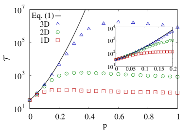
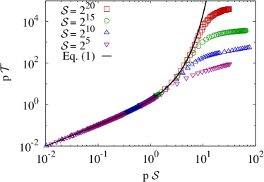
Figure 3: (a) Comparison of the heuristic lifetime from Eq. (1) with simulation data in $d=1$, 2, and 3 for $\mathcal{S}=32$. The inset shows detail for $p<0.2$. (b) Comparison of Eq. (1) expressed in scaled form with simulation data in $d=1$ for $\mathcal{S}$ up to $2^{20}$.

Equation (1) should hold as long as the density of food eaten over the spatial range where the forager wanders throughout its lifespan is small. After $\mathcal{T}$ steps, this spatial range is of the order of $\sqrt{\mathcal{T}}$ in dimension $d=1$. Thus the density of food eaten within this spatial range is of the order of $p\mathcal{T}/\sqrt{\mathcal{T}}=p\sqrt{\mathcal{T}}$, which should be be less than 1 for the assumption of no depletion to be valid. We therefore substitute the lifetime from (1) into $p\sqrt{\mathcal{T}}<1$ to give $\ln(1-p)>(\ln p)/\mathcal{S}$. Expanding the logarithm to lowest order gives $p<-\ln p/\mathcal{S}$, or $p<(\ln\mathcal{S})/\mathcal{S}$. In $d$ dimensions, the density of food eaten after $\mathcal{T}$ steps is given by $p\mathcal{T}/\mathcal{T}^{d/2}$. Requiring this density to be small gives $p<1$ in $d=2$ and no constraint on $p$ for $d>2$. These predictions accord with simulation data for $\mathcal{S}=32$ (Fig. 3(a)), which is the largest value of $\mathcal{S}$ that we can practically simulate in $d=3$, and for $\mathcal{S}$ up to $2^{20}$ in $d=1$ (Fig. 3(b)). The agreement between the data and Eq. (1) holds over a larger range of $p$ as the dimension increases, as follows from our argument.

3 Simulations in One Dimension

We characterize the forager dynamics by its lifetime $\mathcal{T(\mathcal{S}},p)$. The basic feature of the myopic forager is that there is an optimal value of the myopia parameter, $p^{*}(\mathcal{S})$, distinct for each $\mathcal{S}$, that maximizes the forager lifetime (Fig. 4). From plots such as these, we thereby determine the optimal value of $p^{*}(\mathcal{S})$ for $\mathcal{S}$ between $2$ and $2^{20}$ with an accuracy of 1% or less. As shown in Fig. 5(a), the data for the optimal value $p^{*}(\mathcal{S})$ is roughly consistent with $p^{*}\sim 1/\mathcal{S}$, but the data exhibit a slight but decreasing downward curvature. Indeed the functional form $p^{*}\sim\ln\mathcal{S}/\mathcal{S}$ fits the data quite well. Notice that this form for $p^{*}$ also corresponds to the limit of validity of the heuristic approach given in Sec. 2.

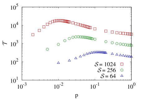
Figure 4: Forager lifetime versus $p$ in $d=1$ for three representative $\mathcal{S}$ values.

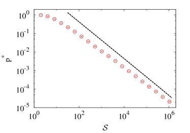
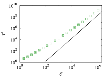
Figure 5: (a) Optimal myopia $p^{*}$ versus $\mathcal{S}$, and (b) maximal lifetime versus $\mathcal{S}$ in $d=1$. The (very thin) error bars are smaller than all data points. The dashed lines have slope $-1$ in (a) and $+2$ in (b). The data are based on $10^{4}$ realizations for $\mathcal{S}\leq 2^{19}$ and $10^{3}$ realizations for $\mathcal{S}=2^{20}$.

Once we determine the optimal value $p^{*}$ for each $\mathcal{S}$, we then study the $\mathcal{S}$ dependence of the lifetime at this optimal myopia $p^{*}(\mathcal{S})$. We define this maximal lifetime as $\mathcal{T}^{*}(\mathcal{S})$. The maximal lifetime is a smoothly increasing function of $\mathcal{S}$ with slow upward curvature on a double logarithmic scale (Fig. 5(b)). This slow curvature again suggests the presence of logarithmic corrections. Indeed, the data for $\ln\mathcal{S}\times\mathcal{T}^{*}$ appears to grow as $\mathcal{S}^{2}$. In fact, substituting the value of $p^{*}\sim\ln\mathcal{S}/\mathcal{S}$ into Eq. (1) also gives $\mathcal{T}^{*}\sim\mathcal{S}^{2}/\ln\mathcal{S}$. Finally, notice that this optimal value of $\mathcal{T}^{*}$ is much larger than the lifetime of the normal forager, which grows as $A\mathcal{S}$, with $A$ exactly calculable and approximately equal to $3.2768$ [1, 2] and also much larger than the limiting $p\to 0$ behavior of $\mathcal{S}=\mathcal{S}$. Thus our heuristic argument predicts that there must be maximum in the forager lifetime as a function of $p$, as well as the $\mathcal{S}$ dependence of the maximal lifetime $\mathcal{T}^{*}$.

We now study the geometry of the desert. Although the desert that is carved out by the forager consists of multiple segments of empty and food-containing sites (Fig. 1), its average density profile has a simple character (Fig. 6). For a forager that starts at $x=0$ and has metabolic capacity $\mathcal{S}$ and myopia parameter $p$, we measure the probability $P(x)$ that food at site $x$ has been consumed up to the instant when the forager starves. The dependence of this probability distribution on $p$ and $\mathcal{S}$ is not written for notational simplicity. Clearly $P(x)$ is decreases with $x$ because it is progressively less likely that the forager reaches a large distance and consumes food there. As shown in Fig. 6, the density profile is an exponentially decaying function of $x$ for all $x$; that is, $P(x)=X^{-1}\exp[-x/X]$, where $X=\langle x(p,\mathcal{S})\rangle$ is the mean extent of the depleted region. Thus the scaling function $f(z)\equiv X\,P(x/X)$ depends only on the scaling variable $z\equiv x/X$, as illustrated in the figure.

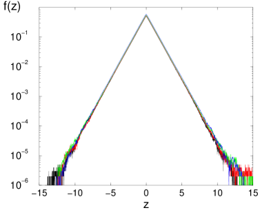
Figure 6: Scaled density profile $f(z)=XP(x/X)$ as a function of $z\equiv x/X$ in $d=1$. The four datasets, each based on $10^{6}$ realizations, are for $p=0.01$ and $\mathcal{S}=327=10^{10/4}$ (black) $563=10^{11/4}$ (red), $1000=10^{12/4}$ (green), and $1779=10^{13/4}$ (blue).

A simple mechanism underlies this exponential behavior of the density profile. Empirically, we find that the distribution of lifetimes $Q(\mathcal{T})$ of the myopic forager has an exponential tail, $Q(\mathcal{T})\sim\exp(-\mathcal{T}/\mathcal{T}^{*})$ in all dimensions. At the instant of starvation the probability that the forager has traveled a distance $r$ from its starting point is just the standard Gaussian $p(x,\mathcal{T})\sim\exp(-r^{2}/4D\mathcal{T})$, where $D$ is the diffusion coefficient of the forager. Convolving this Gaussian with the exponential lifetime distribution $Q(\mathcal{T})$, the outcome is again exponential decay in $x$, as written above. Related convolution-generated non-Gaussian behavior has been obtained in other generalized random walk models [16].

4 Simulations in Greater Than One Dimension

The dynamical behavior of the forager in $d\geq 2$ is qualitatively similar to that in $d=1$. However, because we can simulate only to $\mathcal{S}=2^{10}$ in $d=2$ and to $\mathcal{S}=2^{5}$ in $d=3$, our estimates for asymptotic behavior are imprecise. In $d=2$, the forager lifetime is again maximal at an intermediate value of $p^{*}$ that is strictly between 0 and 1 (Fig. 7) and also is a decreasing function of $\mathcal{S}$ (Fig. 8(a)). The dependence of $p^{*}$ versus $\mathcal{S}$ is almost linear on a double logarithmic scale (based on the last 7 points). A linear least-squares fit of the last 4 data points indicates that $p^{*}\sim\mathcal{S}^{-\alpha}$, with $\alpha\approx 0.76$. While the local slopes of $\ln p^{*}$ versus $\ln\mathcal{S}$ are becoming slightly more negative for larger $\mathcal{S}$, the number of data points is to few to extrapolate with any confidence. Thus we believe that $\alpha\approx 0.8$, with an uncertainty of roughly 0.1.

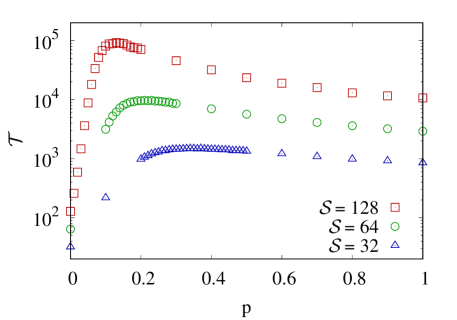
Figure 7: Forager lifetime versus $p$ in $d=2$ for three representative values of $\mathcal{S}$.

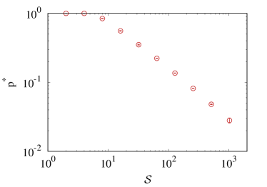
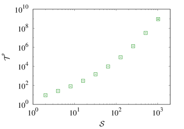
Figure 8: (a) The optimal value of $p$, $p^{*}$, as a function of $\mathcal{S}$, and (b) the maximal forager lifetime, $\mathcal{T}^{*}$, as a function of $\mathcal{S}$ in $d=2$. Error bars are shown. The data is based on $10^{4}$ realizations for $\mathcal{S}\leq 2^{9}$ and $10^{2}$ realizations for $\mathcal{S}=2^{10}$.

The maximal lifetime $\mathcal{T}^{*}$ of the myopic forager in $d=2$ grows much more rapidly with $\mathcal{S}$ than in $d=1$. On a double logarithmic scale, the data show significant upward curvature, which suggests that $\mathcal{T}^{*}$ grows faster than a power law in $\mathcal{S}$. However, a plot of $\ln\mathcal{T}^{*}$ versus $\mathcal{S}$ is curved downward, which excludes exponential growth. The data can be reasonably fit by a fractional exponential, $\mathcal{T}\sim\exp(\mathcal{S}^{\beta})$ with $\beta\approx 0.3$. This behavior roughly accords with Eq. (1): if $p^{*}\sim\mathcal{S}^{-\alpha}$, with $\alpha\approx 0.8$, then Eq. (1) predicts that $\mathcal{T}\sim\exp(\mathcal{S}^{\beta})$, with $\beta=1-\alpha=0.2$. To reach an unambiguous conclusion about the dependence of $\mathcal{T}^{*}$ versus $\mathcal{S}$ would require orders of magnitude longer simulations.

As in the case of $d=1$, the desert that is carved out by a forager in $d=2$ consists of multiple, disjoint food-free regions (Fig. 1(d)). In spite of this complicated geometry for a single trajectory, the average profile of the desert again has a simple character. For a forager that starts at $x=0$ and has metabolic capacity $\mathcal{S}$ and myopia parameter $p$, we measure the density profile $P(\mathbf{r})$ that the food at site $\mathbf{r}$ has been consumed up to the instant that the forager starves. This distribution is again a decreasing function of $|\mathbf{r}|$ because it is progressively less likely that the forager reaches a large distance and consumes food there (Fig. 9). The data indicate that the decay of the density profile is exponential in $\mathbf{r}$, as in the case of one dimension. The mechanism that causes this exponential density profile is the same as that in one dimension.

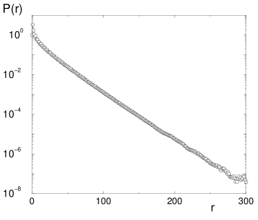
Figure 9: The radial density profile of the desert in $d=2$ for the case of $p=0.4$ and $\mathcal{S}=32$, averaged over $10^{4}$ realizations.

For completeness, we also simulate the myopic forager in $d=3$. Here the maximal lifetime grows so rapidly with $\mathcal{S}$ and the requisite memory needs are so large that we can only simulate the myopic forager for $\mathcal{S}\leq 32$. Figs. 10(a) shows the behavior of the lifetime versus $\mathcal{S}$ up to $\mathcal{S}=32$, while Figures 10(b) and (c), show the dependence of the optimal myopia $p^{*}$ and the maximal lifetime $\mathcal{T}^{*}$ as a function of $\mathcal{S}$. The only claim that we can make from the small range of data is that $\mathcal{T}^{*}$ grows faster than any power law in $\mathcal{S}$.

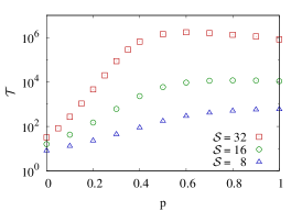
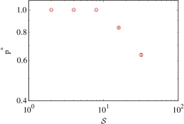
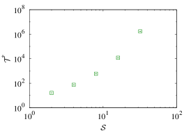
Figure 10: Simulation results in $d=3$. (a) Forager lifetime versus $p$ for three representative $\mathcal{S}$ values. (b) The optimal value of $p$, $p^{*}$, as a function of $\mathcal{S}$, and (c) the maximal forager lifetime, $\mathcal{T}^{*}$, as a function of $\mathcal{S}$. Error bars are shown. The data in (b) and (c) is based on $10^{4}$ realizations for $\mathcal{S}\leq 2^{4}$ and $10^{3}$ realizations for $\mathcal{S}=2^{5}$.

5 Summary

We extended the starving random walk model of foraging to the situation where the forager is myopic and eats with probability $p<1$ when it encounters food. As found previously in a variety of idealized foraging models [9, 10, 11], the forager lifetime is maximized when the basic model parameter, the degree of myopia $p$, is set to an optimal value. This optimal myopia $p^{*}$ appears to scale as $\ln\mathcal{S}/\mathcal{S}$ in one dimension and as $\mathcal{S}^{-\alpha}$ in two dimensions with $\alpha\approx 0.8$. At this optimal myopia, the maximal lifetime appears to grow as $\mathcal{S}^{2}/\ln\mathcal{S}$ in one dimension and as $\exp(\mathcal{S}^{\beta})$ in two dimensions, with $\beta$ close to the value $1-\alpha$, as anticipated from Eq. (1).

An important message from this model is that a forager with a poor ability to detect food lives much longer than a forager with perfect detection capability. This increased lifetime arises because the myopic forager typically eats when it is nutritionally depleted by a significant amount, so that the wastage of food resources is small. In contrast, a normal forager (with $p=1$) always eats when food is encountered and thus may waste a considerable amount of food whenever it eats again soon after its most recent meal. Thus for a naive forager with limited information processing capability, being myopic—equivalently, being somewhat clueless—turns out to be a surprisingly effective survival strategy.

References

- [1] O. Bénichou and S. Redner, Phys. Rev. Lett. 113, 238101 (2014).
- [2] M. Chupeau, O. Bénichou, and S. Redner, J. Phys. A: Math. & Theor. 49, 394003 (2016).
- [3] R. H. MacArthur and E. R. Pianka, Am. Nat. 100, 603 (1966).
- [4] E. L. Charnov, Theor. Popul. Biol. 9, 129 (1976).
- [5] G. H. Pyke, H. R. Pulliam, and E. L. Charnov, Q. Rev. Biol. 52, 137 (1977).
- [6] D. W. Stephens and J. R. Krebs, Foraging Theory, (Princeton University Press, Princeton, NJ, 1986).
- [7] W. J. O’Brien, H. I. Browman, and B. I. Evans, Am. Sci. 78, 152 (1990).
- [8] J. W. Bell, Searching Behaviour, the Behavioural Ecology of Finding Resources, Animal Behaviour Series (Chapman and Hall, London, 1991).
- [9] U. Bhat, S. Redner, and O. Bénichou, Phys. Rev. E 95, 062119 (2017).
- [10] U. Bhat, S. Redner, and O. Bénichou, J. Stat. Mech. 073213 (2017).
- [11] O. Bénichou, U. Bhat, P. L. Krapivsky, and S. Redner, Phys. Rev. E 97, 022110 (2018).
- [12] J. J. Hopfield, Proc. Nat. Acad. Sci. (USA) 71 4135 (1974).
- [13] B. Munsky, G. Bel, and I. Nemenman, J. Chem. Phys. 131, 235103 (2009).
- [14] G. Bel, B. Munsky, and I. Nemenman, Phys. Biol. 7, 016003 (2010).
- [15] S. Redner, A Guide to First-Passage Processes, (Cambridge University Press, Cambridge, UK, 2001).
- [16] A. V. Chechkin, F. Seno, R. Metzler, I. M. Sokolov, Phys. Rev. X 7, 021002 (2017).