A Channel-based Exact Inference Algorithm for Bayesian Networks

Abstract

This paper describes a new algorithm for exact Bayesian inference that is based on a recently proposed compositional semantics of Bayesian networks in terms of channels. The paper concentrates on the ideas behind this algorithm, involving a linearisation (‘stretching’) of the Bayesian network, followed by a combination of forward state transformation and backward predicate transformation, while evidence is accumulated along the way. The performance of a prototype implementation of the algorithm in Python is briefly compared to a standard implementation (pgmpy): first results show competitive performance.

1 Introduction

In general, inference is about answering probabilistic queries of the form: given this-and-this as evidence, what is the likelihood of that? The focus in this paper is on exact inference, where precise answers are sought and not approximations. In general, inference is computationally very expensive. In probabilistic graphical models one can exploit the graph structure in various ways. Here we concentrate on Bayesian networks, whose underlying graphs are directed and acyclic.

This paper presents a new algorithm for (exact) inference in Bayesian networks. The algorithm is based on a novel logical perspective on Bayesian networks, which has its roots in category theory and in the semantics of programming languages. Category theory is a mathematical formalism that concentrates on universal properties of mathematical constructs, see e.g. [2, 15, 13]. In computer science it is especially used to capture the essential structural properties in type theory and programming semantics. Its approach gives a ‘helicopter’ view in which, for instance, the similarities between discrete and continuous probabilistic computation (or even quantum computation) are emphasised [7]. In all these cases one deals with symmetric monoidal categories, for which a graphical language (‘string diagrams’, see e.g. [16]), has been developed. This language exploits the compositional character of this setting, with sequentical composition $\mathbin{\ast}$ interacting appropriately with parallel composition $\otimes$. This string diagram calculus is similar, but subtly different from the graphical languages used for Bayesian networks, see e.g. [5, 9, 10].

Here we shall not go into these underlying categorical theories nor into string diagrams. We refer to [10] for a recent (gentle) introduction. Instead, we present our approach in a rather hands-on manner, via a well-known Bayesian network example from the literature. It is based on the notion of channel, as abstraction of stochastic matrix. In fact, it is shown how conditional probability tables in Bayesian networks can be naturally seen as channels. This is not a novelty, but what is crucial for the current approach, is that along a channel one can do forward transformation $\gg$ of states (distributions), and backward transformation $\ll$ of predicates, see also [8]. These ideas are explained in Sections 2 and 3. There it is also shown how updating of states with predicates (evidence), in combination with forward and backward transformations, allows us to do Bayesian inference at a high level of abstraction, essentially by following the graph structure. We are well aware of the fact that this channel-based formalism deviates from the standard notation and terminology in Bayesian probability. But we do hope that the new algorithm for Bayesian inference that builds on this approach provides enough motivation to look into it.

Indeed, the interpretation of a Bayesian network in terms of channels is essential for the new inference algorithm, which is explained in Section 4. The algorithm consists of three steps: (1) the Bayesian network is stretched to a linear chain of channels; (2a) state transformation is performed forwardly, from the beginning of this chain, to the observation point in the chain, while evidence is incorporated along the way; (2b) predicate transformation is performed backwardly, from the end of the chain, to the observation point, while evidence is accumulated along the way. Finally, at the observation point, the (relevant marginal of the) updated state is returned as output. Section 4 provides more details, including two optimisation steps.

A prototype implementation of this stretch-and-infer algorithm has been written in Python, simply in order to investigate whether the approach works and can handle non-trivial examples. The implementation builds on the EfProb library [4] for channel-based probabilistic computations. This paper concentrates on the methodology to use channel-based compositional semantics for Bayesian inference — the main intellectual contribution — and not on this prototype implementation. Nevertheless, a brief comparison with the standard Variable Elimination algorithm (see e.g. [12, 3, 11]) is given in Subsection 4.4. The comparison is complicated by the level of non-determinism involved in these inference algorithms. Nevertheless, the comparison does indicate that our algorithm can handle non-trivial (standard) examples faster than Variable Elimination in the widely used Python library pgmpy for probabilistic graphical modeling [1].

The computations that have to be performed for inference are in principle well-known, by Bayes’ rule, namely suitable sums and products, and also divisions for normalisation. The cleverness in various algorithms lies in the order in which these computations are performed. In the terminology of Variable Elimination, this means the order in which variables are eliminated. The analogue in our algorithm is the order in which channels are lined-up in a chain, during the first, stretching phase of the computation. This order is randomly produced in a non-deterministic process, through iterations over sets, instead of lists, of ancestors of nodes. However, what we can do is perfom ‘dry runs’ of the stretching in order to find the best order (with the least width), as optimisation of our algorithm, see Subsection 4.3.1.

The outcome of an algorithm should not depend on its non-deterministic choices. In our algorithm this leads to the mathematical question whether the outcome is independent of the ordering of channels in a chain. Section 5 is devoted to answering this question, positively, by reducing the situation to its essential form. Finally, Section 6 describes future work.

2 The channel-based approach to Bayesian networks

This section explains in a concrete way how Bayesian networks can be described conveniently in terms of states $\omega$, channels $c$, and forward transformation $c\gg\omega$ of a state along a channel. For a more elaborate introduction we refer to [10], and to [6] for a more abstract account of the underlying category theory. We shall use the (categorical) calculus of channels, with sequential $\mathbin{\ast}$ and parallel $\otimes$ composition, in order to calculate marginals of a Bayesian network. We use as running example the standard ‘Asia’ Bayesian network, as reproduced in Figure 1. It describes a simple network for medical diagnostics.

Figure 1: The ‘Asia’ example from bnlearn.com with its conditional probability tables

2.1 Sequential composition

We write $t,f$ for the two ‘true’ and ‘false’ elements of the 2-element set $2=\{t,f\}$. The initial nodes smoke and asia in Figure 1 come equipped with two probability distributions on this set $2$. We like to write them as:

$$\begin{array}[]{rclcrcl}\textsf{smoke}&=&0.5|{\kern 1.00006pt}t{\kern 1.00006pt}\rangle+0.5|{\kern 1.00006pt}f{\kern 1.00006pt}\rangle&\qquad\mbox{and}&\textsf{asia}&=&0.01|{\kern 1.00006pt}t{\kern 1.00006pt}\rangle+0.99|{\kern 1.00006pt}f{\kern 1.00006pt}\rangle.\end{array}$$

More generally, a probability distribution on an $n$-element set $X=\{x_{1},\ldots,x_{n}\}$ will be written as formal convex sum $\sum_{i}r_{i}|{\kern 1.00006pt}x_{i}{\kern 1.00006pt}\rangle$ with $r_{i}\in[0,1]$ satisfying $\sum_{i}r_{i}=1$. Such a distribution will often be called a state. We write $\mathcal{D}(X)$ for the set of such distributions/states on $X$. Thus we have $\textsf{smoke},\textsf{asia}\in\mathcal{D}(2)$.

A conditional probability table (CPT) for a node in Figure 1 with $n$ parents corresponds to a function $2^{n}\rightarrow\mathcal{D}(2)$. For instance, we can read off:

$$\begin{array}[]{ccc}\begin{array}[]{rcl}\textsf{lung}(t)&=&0.1|{\kern 1.00006pt}t{\kern 1.00006pt}\rangle+0.9|{\kern 1.00006pt}f{\kern 1.00006pt}\rangle\\ \textsf{lung}(f)&=&0.01|{\kern 1.00006pt}t{\kern 1.00006pt}\rangle+0.99|{\kern 1.00006pt}f{\kern 1.00006pt}\rangle\end{array}&&\begin{array}[]{rcl}\textsf{dysp}(t,t)&=&0.9|{\kern 1.00006pt}t{\kern 1.00006pt}\rangle+0.1|{\kern 1.00006pt}f{\kern 1.00006pt}\rangle\\ \textsf{dysp}(t,f)&=&0.7|{\kern 1.00006pt}t{\kern 1.00006pt}\rangle+0.3|{\kern 1.00006pt}f{\kern 1.00006pt}\rangle\\ \textsf{dysp}(f,t)&=&0.8|{\kern 1.00006pt}t{\kern 1.00006pt}\rangle+0.2|{\kern 1.00006pt}f{\kern 1.00006pt}\rangle\\ \textsf{dysp}(f,f)&=&0.1|{\kern 1.00006pt}t{\kern 1.00006pt}\rangle+0.9|{\kern 1.00006pt}f{\kern 1.00006pt}\rangle\end{array}\end{array}$$

More generally, for sets $X,Y$, a channel from $X$ to $Y$ is a function $X\rightarrow\mathcal{D}(Y)$. It consists of an $X$-indexed collection of states on $Y$. It may be understood as a $\#X\times\#Y$ stochastic matrix. We often write $c\colon X\mathrel{\ooalign{$\to$\cr\hfil\!$\leavevmode\hbox{\set@color \leavevmode\hbox to3.2pt{\vbox to3.2pt{\text{[drawing]}}}}$\hfil\cr}}Y$ when we mean that $c$ is a channel from $X$ to $Y$, and thus a function from $X$ to $\mathcal{D}(Y)$. As we shall see, this special arrow $\mathrel{\ooalign{$\to$\cr\hfil\!$\leavevmode\hbox{\set@color \leavevmode\hbox to3.2pt{\vbox to3.2pt{\text{[drawing]}}}}$\hfil\cr}}$ is convenient when we compose channels, both sequentially and in parallel. Notice by the way that a state/distribution on a set $X$ is in fact also a channel, namely a channel of the form $1\mathrel{\ooalign{$\to$\cr\hfil\!$\leavevmode\hbox{\set@color \leavevmode\hbox to3.2pt{\vbox to3.2pt{\text{[drawing]}}}}$\hfil\cr}}X$, where $1=\{0\}$ is a singleton set.

A very basic operation associated with channels is state transformation. If we have a state $\omega=\sum_{i}r_{i}|{\kern 1.00006pt}x_{i}{\kern 1.00006pt}\rangle$ on $X$, and a channel $c\colon X\mathrel{\ooalign{$\to$\cr\hfil\!$\leavevmode\hbox{\set@color \leavevmode\hbox to3.2pt{\vbox to3.2pt{\text{[drawing]}}}}$\hfil\cr}}Y$, we can form a new state on $Y$, written as $c\gg\omega$. If we write $c(x_{i})=\sum_{j}s_{ij}|{\kern 1.00006pt}y_{ij}{\kern 1.00006pt}\rangle$, then:

$$\begin{array}[]{rcl}c\gg\omega&\coloneqq&\displaystyle\sum_{ij}r_{i}\cdot s_{ij}|{\kern 1.00006pt}y_{ij}{\kern 1.00006pt}\rangle.\end{array}$$

For instance, in the context of the Asia example,

$$\begin{array}[]{rcl}\textsf{lung}\gg\textsf{smoke}&=&0.055|{\kern 1.00006pt}t{\kern 1.00006pt}\rangle+0.9450|{\kern 1.00006pt}f{\kern 1.00006pt}\rangle\\ \textsf{tub}\gg\textsf{asia}&=&0.0104|{\kern 1.00006pt}t{\kern 1.00006pt}\rangle+0.9896|{\kern 1.00006pt}f{\kern 1.00006pt}\rangle.\end{array}$$

Thus, with state transformation $\gg$ we can calculate ‘marginal’ states for nodes in the graph, by just following the path. So far we have done single steps, we can also do this for multiple steps by composing channels sequentially. For channels $c\colon X\mathrel{\ooalign{$\to$\cr\hfil\!$\leavevmode\hbox{\set@color \leavevmode\hbox to3.2pt{\vbox to3.2pt{\text{[drawing]}}}}$\hfil\cr}}Y$ and $d\colon Y\mathrel{\ooalign{$\to$\cr\hfil\!$\leavevmode\hbox{\set@color \leavevmode\hbox to3.2pt{\vbox to3.2pt{\text{[drawing]}}}}$\hfil\cr}}Z$ we can form a composite channel $d\mathbin{\ast}c\colon X\mathrel{\ooalign{$\to$\cr\hfil\!$\leavevmode\hbox{\set@color \leavevmode\hbox to3.2pt{\vbox to3.2pt{\text{[drawing]}}}}$\hfil\cr}}Z$ in the following way. Recall that we have to define $d\mathbin{\ast}c$ as a function $X\rightarrow\mathcal{D}(Z)$. We use state transformation along the channel $d$ in:

$$\begin{array}[]{rcl}\big{(}d\mathbin{\ast}c\big{)}(x)&\coloneqq&d\gg c(x).\end{array}$$

It is not hard to see that this composition is associative. There is an identity channel $\mathrm{id}\colon X\mathrel{\ooalign{$\to$\cr\hfil\!$\leavevmode\hbox{\set@color \leavevmode\hbox to3.2pt{\vbox to3.2pt{\text{[drawing]}}}}$\hfil\cr}}X$ given by $\mathrm{id}(x)=1|{\kern 1.00006pt}x{\kern 1.00006pt}\rangle$, so that $\mathrm{id}\mathbin{\ast}c=c=c\mathbin{\ast}\mathrm{id}$. Further, one has ‘functoriality’ properties:

$$\begin{array}[]{rclcrcl}(d\mathbin{\ast}c)\gg\omega&=&d\gg(c\gg\omega)&&\mathrm{id}\gg\omega&=&\omega.\end{array}$$

We summarise the situation at some higher level of abstraction. Roughly, a Bayesian network consists of a directed acyclic graph (a ‘DAG’) with a conditional probability table for each node. These tables have to be of the right ‘dimension’. Associated with each node $A$ of the network, a finite set $\underline{A}$ is implicitly associated, with at least two elements. We write $\#A$ for the number of elements of $\underline{A}$. Often, $\#A=2$, as in the Asia example, but larger sets are allowed. If the node $A$ has (direct) parent nodes $B_{1},\ldots,B_{n}$, then the conditional probability table associated with $A$ has $\#B_{1}\cdot\ldots\cdot\#B_{n}$ many distributions on $\underline{A}$. Thus we can associate such a node $A$ with a channel $\underline{B}_{1}\times\cdots\times\underline{B}_{n}\mathrel{\ooalign{$\to$\cr\hfil\!$\leavevmode\hbox{\set@color \leavevmode\hbox to3.2pt{\vbox to3.2pt{\text{[drawing]}}}}$\hfil\cr}}\underline{A}$. Channels can be composed sequentially, and states/distributions can be transformed along channels.

2.2 Parallel composition

In a Bayesian network like in Figure 1 certain structure occurs in parallel. For instance, the two initial nodes smoke and asia can be combined into a joint distribution $\textsf{smoke}\otimes\textsf{asia}$ on $2\times 2$. We now describe how such parallel composition $\otimes$ works, both for states and for channels.

Given two states $\omega=\sum_{i}r_{i}|{\kern 1.00006pt}x_{i}{\kern 1.00006pt}\rangle$ on $X$ and $\rho=\sum_{j}s_{j}|{\kern 1.00006pt}y_{i}{\kern 1.00006pt}\rangle$ on $Y$, we can form the ‘joint’ or ‘product’ state $\omega\otimes\rho$ on $X\times Y$, namely:

$$\begin{array}[]{rcl}\omega\otimes\rho&\coloneqq&\displaystyle\sum_{i,j}r_{i}\cdot s_{j}|{\kern 1.00006pt}x_{i},y_{j}{\kern 1.00006pt}\rangle.\end{array}$$

For instance,

$$\begin{array}[]{rcl}\lx@intercol\@ADDCLASS{ltx_eqn_lefteqn}$\displaystyle\textsf{smoke}\otimes\textsf{asia}$\mbox{}\hfil\lx@intercol\\ &=&0.005|{\kern 1.00006pt}t,t{\kern 1.00006pt}\rangle+0.495|{\kern 1.00006pt}t,f{\kern 1.00006pt}\rangle+0.005|{\kern 1.00006pt}f,t{\kern 1.00006pt}\rangle+0.495|{\kern 1.00006pt}f,f{\kern 1.00006pt}\rangle\\ \lx@intercol\@ADDCLASS{ltx_eqn_lefteqn}$\displaystyle(\textsf{lung}\gg\textsf{smoke})\otimes\textsf{asia}$\mbox{}\hfil\lx@intercol\\ &=&0.00055|{\kern 1.00006pt}t,t{\kern 1.00006pt}\rangle+0.0544|{\kern 1.00006pt}t,f{\kern 1.00006pt}\rangle+0.00945|{\kern 1.00006pt}f,t{\kern 1.00006pt}\rangle+0.936|{\kern 1.00006pt}f,f{\kern 1.00006pt}\rangle.\end{array}$$

We extend $\otimes$ from states to channels via a pointwise definition: for $c\colon X\mathrel{\ooalign{$\to$\cr\hfil\!$\leavevmode\hbox{\set@color \leavevmode\hbox to3.2pt{\vbox to3.2pt{\text{[drawing]}}}}$\hfil\cr}}Y$ and $d\colon A\mathrel{\ooalign{$\to$\cr\hfil\!$\leavevmode\hbox{\set@color \leavevmode\hbox to3.2pt{\vbox to3.2pt{\text{[drawing]}}}}$\hfil\cr}}B$ we get $c\otimes d\colon X\times A\mathrel{\ooalign{$\to$\cr\hfil\!$\leavevmode\hbox{\set@color \leavevmode\hbox to3.2pt{\vbox to3.2pt{\text{[drawing]}}}}$\hfil\cr}}Y\times B$ via:

$$\begin{array}[]{rcl}\big{(}c\otimes d\big{)}(x,a)&\coloneqq&c(x)\otimes d(a).\end{array}$$

With parallel composition $\otimes$ we can compute more marginals in Figure 1. For instance, the marginal at the ‘either’ node can be obtained in several equivalent ways as:

$$\begin{array}[]{rcl}\lx@intercol\@ADDCLASS{ltx_eqn_lefteqn}$\displaystyle\big{(}\textsf{either}\mathbin{\ast}(\textsf{lung}\otimes\textsf{tub})\big{)}\gg(\textsf{smoke}\otimes\textsf{asia})$\mbox{}\hfil\lx@intercol\\ &=&\textsf{either}\gg((\textsf{lung}\otimes\textsf{tub})\gg(\textsf{smoke}\otimes\textsf{asia}))\\ &=&\textsf{either}\gg\big{(}(\textsf{lung}\gg\textsf{smoke})\otimes(\textsf{tub}\gg\textsf{asia})\big{)}\\ &=&0.0648|{\kern 1.00006pt}t{\kern 1.00006pt}\rangle+0.935|{\kern 1.00006pt}f{\kern 1.00006pt}\rangle.\end{array}$$

In order to cover the whole network in this way we need to have copy (and projection) channels. We write $\Delta\colon X\mathrel{\ooalign{$\to$\cr\hfil\!$\leavevmode\hbox{\set@color \leavevmode\hbox to3.2pt{\vbox to3.2pt{\text{[drawing]}}}}$\hfil\cr}}X\times X$ for the channel given by $\Delta(x)=1|{\kern 1.00006pt}x,x{\kern 1.00006pt}\rangle$. Similarly, there are projection channels $\pi_{i}\colon X_{1}\times X_{2}\mathrel{\ooalign{$\to$\cr\hfil\!$\leavevmode\hbox{\set@color \leavevmode\hbox to3.2pt{\vbox to3.2pt{\text{[drawing]}}}}$\hfil\cr}}X_{i}$, for $i=1,2$, given by $\pi_{i}(x_{1},x_{2})=1|{\kern 1.00006pt}x_{i}{\kern 1.00006pt}\rangle$. State transformation $\pi_{i}\gg\omega$ corresponds to marginalisation.

There is a convention in Bayesian networks that if a node has multiple outgoing arrows, then the same data is sent over all these wires. This means that there is implicit copying. We need to make this explicit, for a compositional description of Bayesian networks, and use slightly non-standard notation with copying explicit, as on the right in Figure 2.

         

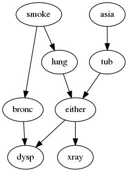
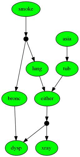
Figure 2: The underlying graph of the Asia example from Figure 1, in standard form on the left, and with explicit copy nodes $\bullet$ on the right.

With this explicit copying in place we see how calculate the marginal for the ‘dysp’ node. It arrises as composition:

$$\begin{array}[]{rcl}\lx@intercol\@ADDCLASS{ltx_eqn_lefteqn}$\displaystyle\big{(}\textsf{dysp}\mathbin{\ast}(\mathrm{id}\otimes\textsf{either})\mathbin{\ast}(\textsf{bronc}\otimes\textsf{lung}\otimes\mathrm{id})\mathbin{\ast}(\Delta\otimes\textsf{tub})\big{)}\gg(\textsf{smoke}\otimes\textsf{asia})$\mbox{}\hfil\lx@intercol\\ &=&0.3975|{\kern 1.00006pt}t{\kern 1.00006pt}\rangle+0.6025|{\kern 1.00006pt}f{\kern 1.00006pt}\rangle.\end{array}\hskip 200.0003pt$$

This state transformation formulation gives a systematic approach to computing marginals, basically by following the graph structure, and translating it into a corresponding channel expression. However, computing the outcome by hand is painful. The EfProb tool [4] has been designed to evaluate such expressions. Without going into details of the EfProb language, we hope the reader sees the correspondence between the above mathematical formula and the EfProb (Python) expression below.

⬇

… >> (smoke @ asia)

0.3975|t> + 0.6025|f>

We challenge the interested reader to write down the channel expression for computing the state for the node xray, and also for the joint state of dysp and xray. One can use the laws:

$$\begin{array}[]{rcl}(d\otimes e)\mathbin{\ast}(c\otimes f)&=&(d\mathbin{\ast}c)\otimes(e\mathbin{\ast}f)\\ (c\otimes d)\gg(\omega\otimes\rho)&=&(c\gg\omega)\otimes(d\gg\rho).\end{array}$$

3 Evidence in Bayesian networks

A typical Bayesian inference question, for the Asia example is: given that a patient has been in Asia and has a positive xray, what is the likelihood of having dyspnea? In this question we have certain ‘evidence’, namely ‘having been in asia’ and ‘positive xray’, and we have a specific ‘observation’ node (namely dysp) whose resulting state we like to infer. This section introduces the machinery to answer such questions under the channel-based interpretation of Bayesian networks.

We take a quite general perspective on evidence, namely using the ‘soft’ or ‘uncertain’ view (using terminology from [3]). Also we use ‘predicate’ instead of ‘evidence’ in line with the terminology from (logical) program semantics, see [10].

Quite generally, a predicate $p$ on a set $X$ is a function $p\colon X\rightarrow[0,1]$. Thus, the truth value $p(x)\in[0,1]$ associated with an element $x\in X$ involves uncertainty. If either $p(x)=0$ or $p(x)=1$, for each $x\in X$, the predicate $p$ is called sharp. A sharp predicate is also called an event. Each set $X$ carries the ‘truth’ predicate $\mathbf{1}\colon X\rightarrow[0,1]$, given by $\mathbf{1}(x)=1$ for each $x\in X$. For two predicates $p,q\colon X\rightarrow[0,1]$ we write $p\mathrel{\&}q$ for the predicate obtained by pointwise multiplication: $(p\mathrel{\&}q)(x)=p(x)\cdot q(x)$. Notice that $p\mathrel{\&}\mathbf{1}=p=\mathbf{1}\mathrel{\&}p$. For the special set $2=\{t,f\}$ we write $\mathit{tt},\mathit{ff}\colon 2\rightarrow[0,1]$ for the (sharp) predicates with $\mathit{tt}(t)=1=\mathit{ff}(f)$ and $\mathit{tt}(f)=0=\mathit{ff}(t)$.

Definition 1

Let $X=\{x_{1},\ldots,x_{n}\}$ be a finite set, with a state $\omega=\sum_{i}r_{i}|{\kern 1.00006pt}x_{i}{\kern 1.00006pt}\rangle$ and a predicate $p\colon X\rightarrow[0,1]$.

1. We write $\omega\models p$ for the validity of predicate $p$ in state $\omega$. It is defined as $\omega\models p\coloneqq\sum_{i}r_{i}\cdot p(x_{i})$. It is the expected value of $p$ in $\omega$.

2. If the validity $\omega\models p$ is non-zero we define an updated state $\omega|_{p}$ on $X$, pronounced as: $\omega$ given $p$. It is defined as:

   $$\begin{array}[]{rcl}\omega|_{p}&\coloneqq&\displaystyle\sum_{i}\frac{r_{i}\cdot p(x_{i})}{\omega\models p}\big{|}{\kern 1.00006pt}x_{i}{\kern 1.00006pt}\big{\rangle}.\end{array}$$

As we see, the updated state $\omega|_{p}$ takes the evidence $p$ into account via multiplication with the probabilities of $\omega$. The resulting values have to be normalised, via the validity $\omega\models p$, in order to obtain a distribution again. We refer to [10] for more information about this updating, including an associated version of Bayes’ rule.

We need one more notion before we can start doing inference, namely predicate transformation along a channel. Given a channel $c\colon X\mathrel{\ooalign{$\to$\cr\hfil\!$\leavevmode\hbox{\set@color \leavevmode\hbox to3.2pt{\vbox to3.2pt{\text{[drawing]}}}}$\hfil\cr}}Y$ and a predicate $q$ on $Y$, we can form a new predicate $c\ll q$ on $X$, via the definition:

$$\begin{array}[]{rclcrcl}\big{(}c\ll q\big{)}(x)&\coloneqq&\displaystyle\sum_{j}s_{j}\cdot p(y_{j})&\qquad\mbox{when}&c(x)&=&\displaystyle\sum_{j}s_{j}|{\kern 1.00006pt}y_{j}{\kern 1.00006pt}\rangle.\end{array}$$

Below we describe some of the mathematical laws that predicate transformation satisfies, but first we like to illustrate how it is used in inference. Let’s ask ourselves a first question. Suppose that we have evidence that a patient has lung cancer; what is then the likelihood of bronchitis?

We proceed in the following methodological way, using that there is a path from nodes ‘lung’ to ‘bronc’ via the initial state ‘smoke’. We have the lungcancer evidence in the form of the predicate $\mathit{tt}$ on the codomain of the lung channel. We first turn it into a predicate $\textsf{lung}\ll\mathit{tt}$ on its domain, and then use it to update the smoke state to $\textsf{smoke}|_{\textsf{lung}\ll\mathit{tt}}$. The answer is obtained via state transformation along the bronc channel:

$$\begin{array}[]{rcl}\textsf{bronc}\gg\big{(}\textsf{smoke}|_{\textsf{lung}\ll\mathit{tt}}\big{)}&=&0.5727|{\kern 1.00006pt}t{\kern 1.00006pt}\rangle+0.4273|{\kern 1.00006pt}f{\kern 1.00006pt}\rangle.\end{array}$$

In the beginning of this section we had a more challenging question, namely: given a visit to Asia and a negative xray, what is the likelihood of dyspnea? For the answer we update the asia state to $\textsf{asia}|_{\mathit{tt}}$ and also update the either state with predicate $\textsf{xray}\ll\mathit{ff}$, and then use these updated states in the forward recomputation of the dyspnea likelihood. In EfProb this looks as follows — where @ is written for the tensor $\otimes$ and / for conditioning.

⬇

… ((copy >> smoke) @ (asia / tt))) / (one @ (xray << ff))

0.3669|t> + 0.6331|f>

Clearly, this answer is not easy to read (and construct). The main contributions of this paper is an algorithm for doing this systematically, by first ‘stretching’ a Bayesian network to a chain of channels, as in Figure 3, and then doing forward & backward inference along this chain. This will be described in the next section.

But before stopping here we would like to write down some basic laws for predicate transformation:

$$\begin{array}[]{rclcrclcrcl}(d\mathbin{\ast}c)\ll q&=&c\ll(d\ll q)&&\mathrm{id}\ll q&=&q&&c\ll\mathbf{1}&=&\mathbf{1}.\end{array}$$

Further, the validity $c\gg\omega\models q$ is the same as $\omega\models c\ll q$. Finally, we mention that causal reasoning (or prediction) is given by first updating and then doing forward state tranformation, as in $c\gg(\omega|_{p})$. In contrast, evidential reasoning (or explanation) involves first doing predicate transformation and then updating, as in $\omega|_{c\ll q}$. We refer to [9, 10] for further details — where these two approaches are called forward and backward inference.

4 A channel-based inference algorithm

Having seen the basics of state transformation, predicate transformation, and state updates, we can now proceed to the novelty of this paper, namely a new channel-based inference algorithm for exact Bayesian inference. The algorithm contains two steps, which we call ‘stretching’ and ‘transformation’ respectively. A prototype version of this algorithm has been developed in Python, on the basis of the EfProb library [4]. It will be described as we proceed. In the end there is a non-rigorous comparison to the standard variable elimination algorithm for inference, as implemented in the widely used pgmpy library for probabilistic graphical modeling. This section will thus have the following subsections.

1. Stretching

2. Transformations

3. Optimisation

4. Comparison.

Figure 3: A stretching of the Asia Bayesian network, producing a chain of channels. The order of the channels with bronc, lung, tub does not matter because of Equation (1); the same holds for dysp and xray.

4.1 Stretching a Bayesian network

The aim of the stretching algorithm is to turn a Bayesian network into a linear chain of channels, with one node (conditional probability table, seen as channel) per step in the chain. Informally, the algorithm works as follows. It first adds initial nodes to the chain. It then adds one by one nodes (as channels in EfProb) all of whose ancestors are already in the chain. For instance, in the Asia example from Figure 2 we can add nodes/channels in a chain in the following orders.

• smoke, asia, bronc, lung, tub, either, dysp, xray

• asia, smoke, tub, lung, either, xray, bronc, dysp

Clearly, there are different possible orders in such a ‘stretched’ chain. When constructing a chain of channels we have to make sure that the inputs are copied and re-arranged when needed. Figure 3 describes the resulting chain of channels corresponding to the first order given above, in which the initial states have been omitted. Recall that we write $2=\{t,f\}$ for the two element set.

At this stage we do not care which order is chosen — although we will have to say a bit more about this later in Subsection 4.3 from an optimisation perspective. From a mathematical perspective the order does not matter so much because we have the following property for channel composition:

$$\begin{array}[]{rcl}(c\otimes\mathrm{id})\mathbin{\ast}(\mathrm{id}\otimes d)&=&(\mathrm{id}\otimes d)\mathbin{\ast}(c\otimes\mathrm{id}).\end{array}$$ (1)

This means that channels that do not interact can be shifted, see Figure 3. There is a bit more to say about this when it comes to updating, but that will be postponed to Section 5.

This stretching algorithm has been implemented in Python. It turns a Bayesian model formalised in the pgmpy library into a chain of composable EfProb channels. The program typically yields different outcomes for different runs. This non-determinism arises because the program iterates over sets (instead of lists) of parent nodes in a pgmpy model; in iterations over sets, a random order is chosen. The implementation involves quite a bit of bookkeeping, in order to copy nodes along the way and to swap inputs so that they are lined up in the right order for the subsequent channel. We are not going to describe these details here. We just like to mention that we do the copying ‘lazily’ in order to keep the size of intermediate sets limited. Recall that taking a parallel product $\otimes$ of distributions involves a multiplication of the sizes of the underlying sets.

Figure 4 gives an impression of two different outcomes of stretching the standard ‘Child’ Bayesian network. It clearly shows that copying is done only when needed. The graphs on the left and right are not properly linear, but this is due to the way such graphs are rendered (using pydot). The underlying datastructures are linear chains of channels.

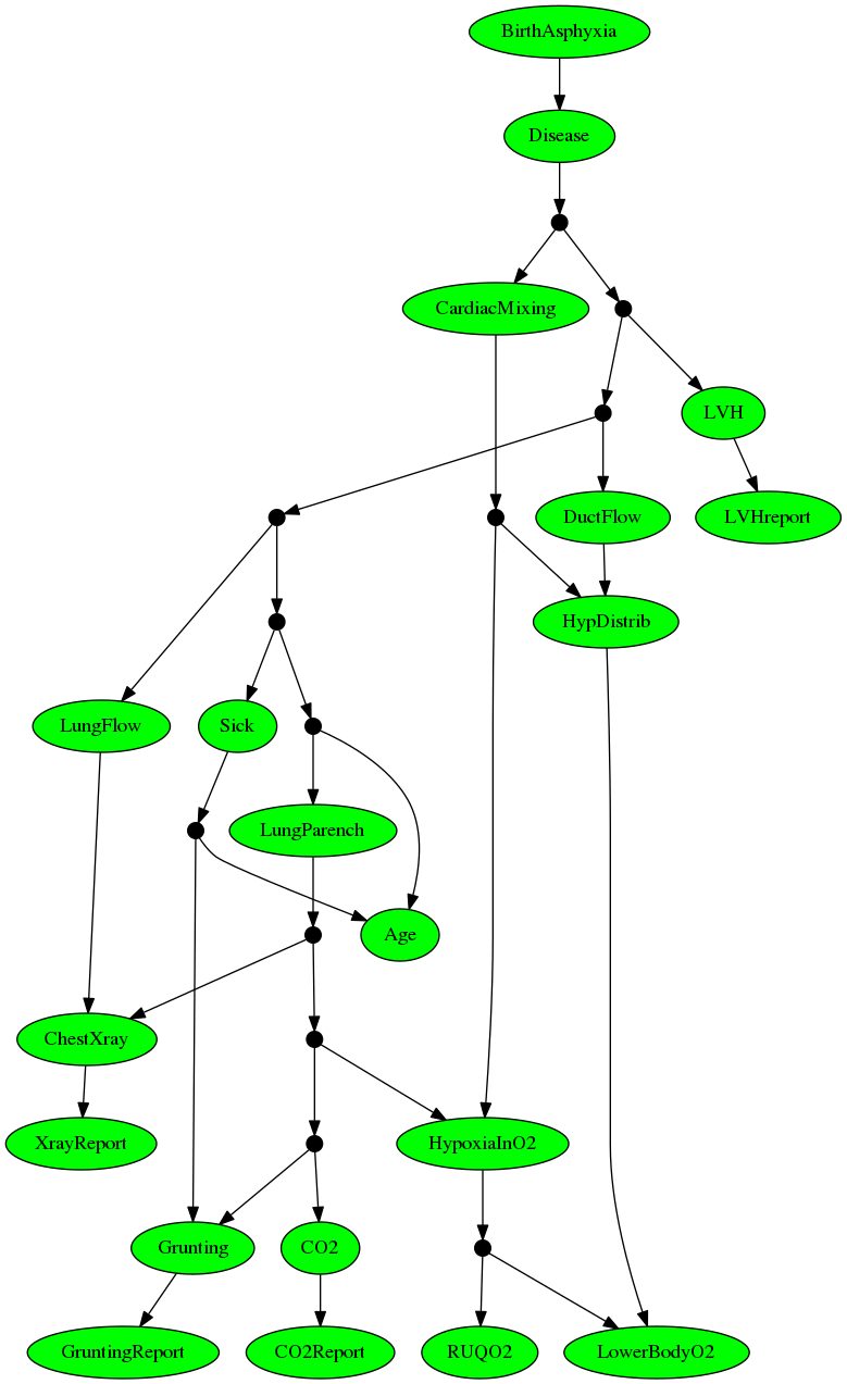
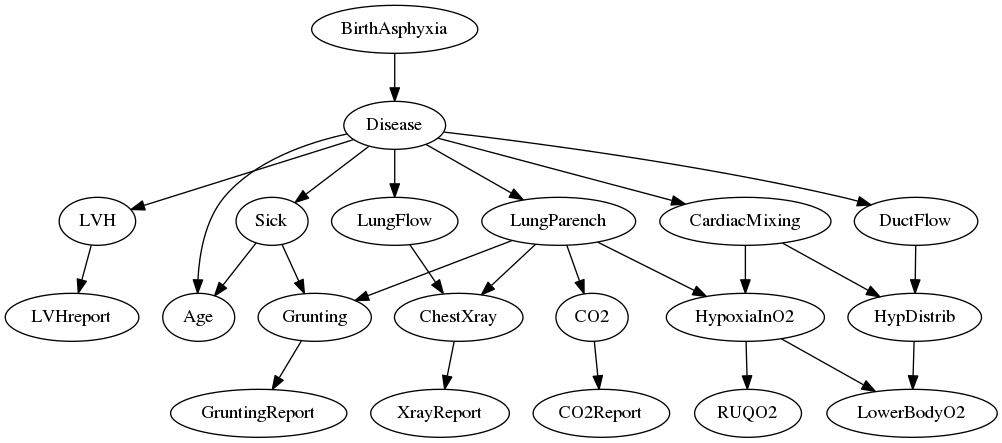
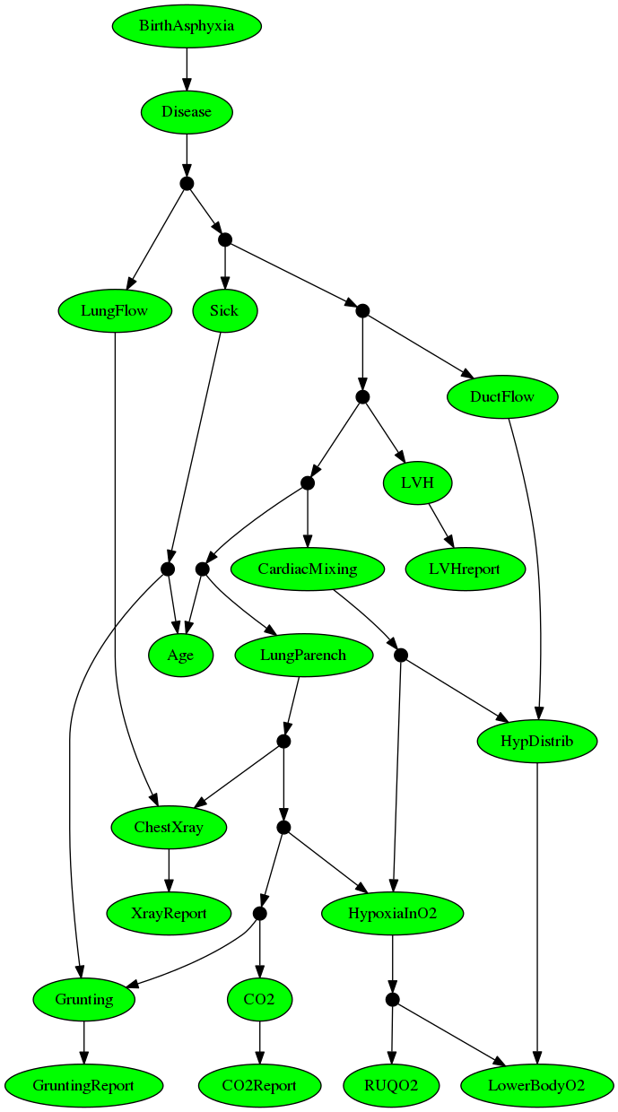
Figure 4: The original ‘Child’ Bayesian network from bnlearn.com in the middle, and two different ways of stretching it, on the left and on the right.

4.2 Transformation along the chain of channels and updating

Figure 5: A stretched Bayesian network with the observation and evidence located somewhere along the chain of channels.

At this stage we are ready to handle inference, as a second step in the algorithm, after stretching. First, we fix the kind of inference queries we will be using, following rather standard practices. Our queries will be of the form:

$$Q\big{(}\mathcal{B},on,en_{1}:p_{1},\ldots,en_{n}\colon p_{1}\big{)}$$ (2)

where:

• $\mathcal{B}$ is the Bayesian network that the query is applied to;

• $on$ is the ‘observation node’;

• $en_{1},\ldots,en_{n}$ are evidence nodes, with predicates $p_{1},\ldots,p_{n}$ on the underlying sets of these nodes.

In the current context we allow the predicates to be fuzzy (soft); this goes beyond existing approaches.

Our inference algorithm, represented in (2) above as a query $Q$, performs the following consecutive steps.

1. Stretch the Bayesian network $\mathcal{B}$ to a linear chain of channels, as described in the previous subsection.

2. Locate the observation node and the evidence nodes at the right stages in this chain, where these nodes appear for the first time as codomain (outcome) of the corresponding channel. The resulting situation is sketched in Figure 5.

3. Perform state transformation from the initial node to the observation node, while updating the state with evidence along the way.

   More concretely, take as first state $\omega_{1}=\textsf{initial}$. Given state $\omega_{i}$ at stage $i$ with subsequent channel $i$, take:

   $$\begin{array}[]{rcl}\omega_{i+1}&\coloneqq&\left\{\begin{array}[]{ll}c_{i}\gg\big{(}\omega_{i}|_{p}\big{)}&\mbox{if there is predicate $p$ at stage $i$ in the chain}\\ c_{i}\gg\omega_{i}&\mbox{otherwise.}\end{array}\right.\end{array}$$

   We continue doing this until the ‘observe’ node point is reached in the chain, from above. The state obtained so far is called $\omega$.

   (There is a subtlety that the predicate $p$ should be suitably weakenend to be of the right type. The same holds for the predicate $p$ in the next point; we ignore these matters at this stage; a precise description is given in Example 2 below.)

4. Perform predicate transformation from the final node to the the observation node, accumulating evidence along the way.

   More concretely, take as predicate $q_{n}=\mathbf{1}$, where $n$ is the length of the chain. If there happens to be evidence with predicate $p$ at the last stage, we take $q_{n}=p$ instead. Assume predicate $q_{i+1}$ is given at stage $i+1$. A new predicate $q_{i}$ is formed for the previous stage, via:

   $$\begin{array}[]{rcl}q_{i}&\coloneqq&\left\{\begin{array}[]{ll}\big{(}c_{i+1}\ll q_{i+1}\big{)}\mathrel{\&}p&\mbox{if there is predicate $p$ at stage $i$ in the chain}\\ c_{i+1}\ll q_{i+1}&\mbox{otherwise.}\end{array}\right.\end{array}$$

   (We recall that $\mathrel{\&}$ is used for pointwise multiplication of fuzzy predicates.) We continue doing this until we reach the observation node, this time from below. Write $q$ for the predicate that has been built up at that point.

5. Return the updated state $\omega|_{q}$, marginalised appropriately to node $on$. This is the output of the inference algorithm. Marginalisation is needed because the underlying set of the state $\omega$ is typically a product of several spaces.

In the code fragment below we illustrate how this looks like for the query that we considered in the previous section: dyspnea likelihood given presence in Asia and negative xray. First we load the Asia Bayesian network from the bnlearn library, in bif format, and turn it into a Bayesian model in pgmpy.

⬇

>>> asia_model = reader.get_model()

Our new algorithm’s answer to the inference query is produced via the function stretch_and_infer, with appropriate arguments:

⬇

… {’asia’ : [1,0], ’xray’ : [0,1]})

0.3669|dysp_0> + 0.6331|dysp_1>

For comparison, using pgmpy’s variable elimination one writes:

⬇

>>> asia_inference.query([’dysp’],

… evidence={’asia’ : 0, ’xray’ : 1})[’dysp’] )

The latter produces the same distribution, but pretty-printed differently:

As mentioned, our implementation allows the use of fuzzy, non-sharp predicates, expressing uncertainly about the evidence at hand, as in:

⬇

… {’asia’ : [0.9, 0.2], ’xray’ : [0.1, 0.75]})

0.3711|dysp_0> + 0.6289|dysp_1>

Example 2

We also describe more concretely how inference along a chain of channels works in the new algorithm. We use the same query as above, applied to the chain of channels described in Figure 3. We use the language EfProb. First, a state forward is defined via state transformation $\gg$, as in step (3) in the above description of the algorithm, where the evidence tt of having been in asia is incorporated immediately at the first step. The observation node is after the dysp channel, so that we can follow the chain in Figure 3 in a step-by-step manner:

⬇

… * (id @ copy)

… * (id @ either)

… * (id @ id @ tub)

… * (id @ lung @ id)

… * (bronc @ id @ id)

… * (copy @ id)

… >> ((smoke @ asia) / (one @ tt))

Notice that the evidence tt (of having been in asia) on the set $2$ is weakened to a predicate one @ tt on $2\times 2$, so that the types match.

Similarly, a predicate backward is defined by starting at the end of the chain, as in step (4) of the algorithm. In this case the negative-xray evidence ff is present at the last point of the chain, and only one predicate transformation step $\ll$ is needed to reach the observation point (after dysp), see again Figure 3.

We are now ready to produce the outcome, in step (5) of the algorithm, via state update and marginalisation (using state transformation with the first projection pi1):

⬇

0.3669|t> + 0.6331|f>

In principle, the stretch step of our inference algorithm can be executed once, as a precomputation. Subsequent multiple queries can then be run on this stretched network. However, in the next subsection we discuss an optimisation step which is query-dependent and make such pre-computation pointless.

4.3 Optimisation of the inference algorithm

The implementation that we have developed for the above inference algorithm is a prototype. Squeezing out the last cycle for efficiency has not been a design goal. Nevertheless, two optimisations have been included, which improve the algorithm as sketched in the previous two subsections.

4.3.1 Doing dry runs first

As we described in Subsection 4.1, stretching of a Bayesian network is a non-deterministic process. From a mathematical perspective, it does not matter which order of channels appears in the resulting chain. However, from a computational perspective it is important to keep the ‘width’ of the chain as small as possible. This width is defined as the maximum size of intermediate product sets in the chain. For instance, in the stretching in Figure 3 the maximal width is 8, given by the 8-element set $2\times 2\times 2$. Different orderings of channels in a chain can lead to different widths.

What our implementation does is perform a number of random ‘dry’ stretch runs, say 1000, to find out in a brute force manner which of these chains has the least width. This is the one that we proceed with, in order to fill in the precise ‘burocratic’ details about coping and swapping in order to line up inputs appropriately for each channel. As an illustration, doing 100 dry runs on the Child network (in the middle of Figure 4) yields the following 28 different possible widths (duplicate occurrences have been removed).

$${\begin{array}[]{lclclcl}19440&&9720&&38880&&4860\\ 7776&&3888&&15552&&12960\\ 6480&&3240&&58320&&8640\\ 23328&&46656&&25920&&5184\\ 11664&&5832&&3456&&77760\\ 2592&&51840&&4320&&116640\\ 93312&&3456&&11520&&17280\end{array}}$$

The smallest width — 2592 in this case — is selected for the remainder of the algorithm. Doing such dry runs is computationally cheap, and well worth spending a little bit of time on, since the variation in widths is substantial.

Instead of these brute force ‘dry’ runs one could use some more clever graph analysis techniques. Such improvements may be added at a later stage; they are besides the main focus of this paper, namely the application of state/predicate transformer semantics in inference.

4.3.2 Pruning the Bayesian network first

An inference query as in (2) contains several nodes, namely for observation ($on$) and for evidence ($en_{i}$). These nodes occur at specific parts in the Bayesian network $\mathcal{B}$ at hand. This means that there are parts of the network which are irrelevant for the inference query. Specifically, if there is a node $n$ in the network and neither the observation node $on$ nor any of the evidence nodes $en_{i}$ occurs in the subnetwork of children of $n$ (including $n$ itself), then $n$ may as well be removed. This is what we apply in our inference algorithm, to the pgmpy model, before it is stretched.

This ‘pruning’ of the Bayesian network, by removing irrelevant nodes, greatly improves the efficiency. But it makes the whole inference algorithm query dependent. Hence the idea that the chain of channels can be pre-computed does not work anymore with this optimisation step.

4.4 Comparison with variable elimination in pgmpy

The aim of the prototype implementation of our channel-based inference algorithm is mainly to see if the idea of reasoning up and down a chain of channels works. We can surely say that it does, from a functional perspective. We have compared it to the standard variable elimination algorithm for inference, as implemented in pgmpy. In all our tests, the outcomes have been the same.

We have also done some performance comparisons. The results described below do give some indication, but not much more than that. For instance, we have only compared to variable elimination in pgmpy, and not to other implementations. Also, the comparison is complicated by the fact that our inference algorithm is non-deterministic — and it seems, variable elimination in pgmpy too. Hence the only thing we can do is compare many runs, on different queries. Here are some findings.

• On small examples, like Asia from Section 2, there is no noticeable timing difference. This Asia model involves 8 nodes and 18 parameters.

• On examples like the Child network from Figure 4, with 20 nodes and 230 parameters, there are clear differences. We have run many randomly generated queries, with between 1 and 5 evidence nodes. On average, on this example, our algorithm is in the order of 10 times faster, on an ordinary laptop. Even with larger numbers of runs, substantial variation in execution times remain. This variation occurs in particular for variable elimination, not for the new algorithm.

• For larger Bayesian networks from bnlearn, like Insurance with 27 nodes and 984 parameters, our inference algorithm often takes about a second to terminate, whereas variable elimination in pgmpy is typically hundreds or even thousands of times slower. We have done these experiments both on a laptop and on a quad processor machine with 3 TiB RAM.

• For even larger networks, like Hailfinder with 2656 parameters, our algorithm fails, because of lack of memory, on the big 3 TiB RAM machine.

5 Irrelevance of channel ordering

In subsection 4.1 we have made a casual remark about stretching a Bayesian network, namely that from a mathematical perspective, the order of channels in a chain does not matter. Actually, there is something to prove here, when we do conditioning. Consider the situation sketched in Figure 5. It may happen that in one ordering of channels a particular piece of evidence (predicate) is above (before) the observation point, whereas in another ordering it is below (after). According to steps 3 and 4 in Subsection 4.2 this predicate will then be treated differently: if it occurs above, the predicate will be incorporated in the final outcome via state transformation; if it occurs below, the predicate will be handled via predicate transformation. We need to show that this yields the same outcomes.

Emperically, we know from running the algorithm multiple times that the outcome is independent of such orderings. But we better prove this mathematically. The theorem below abstracts the situation to its essential form.

Theorem 3

Let $c\colon A\mathrel{\ooalign{$\to$\cr\hfil\!$\leavevmode\hbox{\set@color \leavevmode\hbox to3.2pt{\vbox to3.2pt{\text{[drawing]}}}}$\hfil\cr}}X$ and $d\colon B\mathrel{\ooalign{$\to$\cr\hfil\!$\leavevmode\hbox{\set@color \leavevmode\hbox to3.2pt{\vbox to3.2pt{\text{[drawing]}}}}$\hfil\cr}}Y$ be channels, together with a joint state $\omega\in\mathcal{D}(A\times X)$ and a predicate $q\colon Y\rightarrow[0,1]$ on $Y$. Then the following distributions are the same.

$$\begin{array}[]{rcl}\lx@intercol\@ADDCLASS{ltx_eqn_lefteqn}$\displaystyle\pi_{1}\gg\Big{(}\big{(}(c\otimes\mathrm{id})\gg\omega\big{)}\big{|}_{(\mathrm{id}\otimes d)\ll(\mathbf{1}\otimes q)}\Big{)}$\mbox{}\hfil\lx@intercol\\ &=&\pi_{1}\gg\Big{(}(c\otimes\mathrm{id})\gg\big{(}((\mathrm{id}\otimes d)\gg\omega)\big{|}_{\mathbf{1}\otimes q}\big{)}\Big{)}.\end{array}$$ (3)

This equation deserves some explanation. The outer operation $\pi_{1}\gg(-)$ performs marginalisation, for observing the outcome in $X$. In the upper expression the channel $d$ is used for predicate transformation after using $c$ for state transformation. In the lower expression $d$ is used for state transformation, before applying $c$, also for state transformation, to an updated state. In the style of Figure 5, the upper expression in (3) captures the situation on the left below, whereas the lower expression in (3) is about the picture on the right:

This shows that channels $c$ and $d$ can be shifted along each other in a non-interacting manner, in the presence of conditioning with predicate $q$

• For convenience we shall identify a distribution $\rho\in\mathcal{D}(Z)$ with a function $\rho\colon Z\rightarrow[0,1]$, in a standard manner: if $Z=\{z_{1},\ldots,z_{n}\}$ and $\rho$ is $\sum_{i}r_{i}|{\kern 1.00006pt}z_{i}{\kern 1.00006pt}\rangle$, then $\rho\colon Z\rightarrow[0,1]$ is given by $\rho(z_{i})=r_{i}$. Thus, for $x\in X$,

  $$\begin{array}[b]{rcl}\lx@intercol\@ADDCLASS{ltx_eqn_lefteqn}$\displaystyle\pi_{1}\gg\big{(}\big{(}(c\otimes\mathrm{id})\gg\omega\big{)}\big{|}_{(\mathrm{id}\otimes d)\ll(\mathbf{1}\otimes q)}\big{)}(x)$\mbox{}\hfil\lx@intercol\\ &=&\displaystyle\sum_{b\in B}\big{(}\big{(}(c\otimes\mathrm{id})\gg\omega\big{)}\big{|}_{(\mathrm{id}\otimes d)\ll(\mathbf{1}\otimes q)}\big{)}(x,b)\\ &=&\displaystyle\sum_{b\in B}\frac{((c\otimes\mathrm{id})\gg\omega)(x,b)\cdot((\mathrm{id}\otimes d)\ll(\mathbf{1}\otimes q))(x,b)}{(c\otimes\mathrm{id})\gg\omega\models(\mathrm{id}\otimes d)\ll(\mathbf{1}\otimes q)}\\ &=&\displaystyle\sum_{b\in B}\frac{\big{(}\sum_{a\in A}c(a)(x)\cdot\omega(a,b)\big{)}\cdot\big{(}\sum_{y\in Y}d(b)(y)\cdot q(y)\big{)}}{(\mathrm{id}\otimes d)\gg\omega\models(c\otimes\mathrm{id})\ll(\mathbf{1}\otimes q)}\\ &=&\displaystyle\sum_{y\in Y}\sum_{a\in A}\sum_{b\in B}\frac{c(a)(x)\cdot\omega(a,b)\cdot d(b)(y)\cdot q(y)}{(\mathrm{id}\otimes d)\gg\omega\models(c\ll\mathbf{1})\otimes(\mathrm{id}\ll q)}\\ &=&\displaystyle\sum_{y\in Y}\sum_{a\in A}\frac{c(a)(x)\cdot\big{(}\sum_{b\in B}d(b)(y)\cdot\omega(a,b)\big{)}\cdot q(y)}{(\mathrm{id}\otimes d)\gg\omega\models\mathbf{1}\otimes q}\\ &=&\displaystyle\sum_{y\in Y}\sum_{a\in A}c(a)(x)\cdot\frac{((\mathrm{id}\otimes d)\gg\omega)(a,y)\cdot(\mathbf{1}\otimes q)(a,y)}{(\mathrm{id}\otimes d)\gg\omega\models\mathbf{1}\otimes q}\\ &=&\displaystyle\sum_{y\in Y}\sum_{a\in A}c(a)(x)\cdot\big{(}((\mathrm{id}\otimes d)\gg\omega)\big{|}_{\mathbf{1}\otimes q}\big{)}(a,y)\\ &=&\displaystyle\sum_{y\in Y}\big{(}(c\otimes\mathrm{id})\gg\big{(}((\mathrm{id}\otimes d)\gg\omega)\big{|}_{\mathbf{1}\otimes q}\big{)}\big{)}(x,y)\\ &=&\pi_{1}\gg\big{(}(c\otimes\mathrm{id})\gg\big{(}((\mathrm{id}\otimes d)\gg\omega)\big{|}_{\mathbf{1}\otimes q}\big{)}\big{)}(x).\end{array}$$

6 Concluding remarks

This paper concentrates on the underlying semantical ideas for a new algorithm for exact Bayesian inference. It builds on ideas from (probabilistic) programming semantics, using the notion of channels as primitive, both for state transformation and predicate transformation. The comparison of the prototype implementation of the algorithm in Python to a standard implementation (from pgmpy) gives a first indication, but clearly requires a more systematic analysis, involving different inference algorithms and different implementations. This is beyond the focus of the current paper.

Since the approach is based on a very general underlying semantics, it can be extended in principle also to continuous probability theory. Categorically, this amounts to using the Giry monad $\mathcal{G}$ instead of the distribution monad $\mathcal{D}$, see [7] for details. Even more, it could apply to hybrid networks, combinining both discrete and continuous probability (see [4] for an example). Even more, the approach could be extended to quantum Bayesian probability, since channels (also called superoperators, see [14] or [6]) are a primitive notion in quantum computing too.

Another avenue for further work is to apply the stretching techniques described here also to MAP-inference. This is ongoing work.

Acknoledgements

Thanks are due to Kenta Cho, Fabio Zanasi and Marco Gaboardi for discussions and feedback.

References

• [1] A. Ankand and A. Panda. Mastering Probabilistic Graphical Models using Python. Packt Publishing, Birmingham, 2015.
• [2] S. Awodey. Category Theory. Oxford Logic Guides. Oxford Univ. Press, 2006.
• [3] D. Barber. Bayesian Reasoning and Machine Learning. Cambridge Univ. Press, 2012. Publicly available via http://web4.cs.ucl.ac.uk/staff/D.Barber/pmwiki/pmwiki.php?n=Brml.HomePage.
• [4] K. Cho and B. Jacobs. The EfProb library for probabilistic calculations. In F. Bonchi and B. König, editors, Conference on Algebra and Coalgebra in Computer Science (CALCO 2017), volume 72 of LIPIcs. Schloss Dagstuhl, 2017.
• [5] B. Fong. Causal theories: A categorical perspective on Bayesian networks. Master’s thesis, Univ. of Oxford, 2012. see arxiv.org/abs/1301.6201.
• [6] B. Jacobs. New directions in categorical logic, for classical, probabilistic and quantum logic. Logical Methods in Comp. Sci., 11(3), 2015. See https://lmcs.episciences.org/1600.
• [7] B. Jacobs. From probability monads to commutative effectuses. Journ. of Logical and Algebraic Methods in Programming, 94:200–237, 2017.
• [8] B. Jacobs. A recipe for state and effect triangles. Logical Methods in Comp. Sci., 13(2), 2017. See https://lmcs.episciences.org/3660.
• [9] B. Jacobs and F. Zanasi. A predicate/state transformer semantics for Bayesian learning. In L. Birkedal, editor, Math. Found. of Programming Semantics, number 325 in Elect. Notes in Theor. Comp. Sci., pages 185–200. Elsevier, Amsterdam, 2016.
• [10] B. Jacobs and F. Zanasi. The logical essentials of Bayesian reasoning. See arxiv.org/abs/1804.01193, 2018.
• [11] F. Jensen and T. Nielsen. Bayesian Networks and Decision Graphs. Statistics for Engineering and Information Science. Springer, $2^{\textrm{nd}}$ rev. edition, 2007.
• [12] D. Koller and N. Friedman. Probabilistic Graphical Models. Principles and Techniques. MIT Press, Cambridge, MA, 2009.
• [13] S. Mac Lane. Categories for the Working Mathematician. Springer, Berlin, 1971.
• [14] M. Nielsen and I. Chuang. Quantum Computation and Quantum Information. Cambridge Univ. Press, 2000.
• [15] B. Pierce. Basic Category Theory for Computer Scientists. MIT Press, Cambridge, MA, 1991.
• [16] P. Selinger. A survey of graphical languages for monoidal categories. In B. Coecke, editor, New Structures in Physics, number 813 in Lect. Notes Physics, pages 289–355. Springer, Berlin, 2011.