Single- and two-nucleon momentum distributions for local chiral interactions

Abstract

We present quantum Monte Carlo calculations of the single- and two-nucleon momentum distributions in selected nuclei for $A\leq 16$. We employ local chiral interactions at next-to-next-to-leading order. We find good agreement at low momentum with the single-nucleon momentum distributions derived for phenomenological potentials. The same agreement is found for the integrated two-nucleon momentum distributions at low relative momentum $q$ and low center-of-mass momentum $Q$. We provide results for the two-nucleon momentum distributions as a function of both $q$ and $Q$. The large ratio of $pn$ to $pp$ pairs around $q=2\,\rm fm^{-1}$ for back-to-back $(Q=0)$ pairs is confirmed up to [16]O, and results are compatible with those extracted from available experimental data.

I Introduction

Quantum Monte Carlo (QMC) methods have been extensively used in the past to derive properties of strongly correlated systems, including nuclei, neutron drops, and neutron and nuclear matter (see Ref. Carlson et al. (2015) for a recent review). Part of their success relies on the possibility to tackle the nuclear many-body problem in a nonperturbative fashion, by employing accurate wave functions that include two- and three-body correlations.

Momentum distributions of individual nucleons and nucleon pairs strongly depend on such correlations, as they reflect features of the short-range structure of nuclei. While these momentum distributions are not directly observable, because they are coupled with, e.g., electromagnetic current operators, they do provide a strong influence on some observables such as back-to-back nucleons measured in quasielastic scattering. For instance, it was found that the strong spatial-spin-isospin correlations induced by the tensor force lead to large differences in the $pp$ and $pn$ distributions at moderate values of the relative momentum in the pair Schiavilla et al. (2007); Alvioli et al. (2008). These differences have been observed in $(e,e^{\prime}pN)$ experiments on [12]C at low momentum Subedi et al. (2008) and on [4]He at higher momentum Korover et al. (2014) at Jefferson Laboratory (JLab). The same conclusions have been found in heavier systems, including [27]Al, [56]Fe, and [208]Pb Hen et al. (2014).

The variational Monte Carlo (VMC) method has been used to calculate the momentum distributions in $A\leq 12$ nuclei Schiavilla et al. (1986, 2007); Wiringa et al. (2008, 2014); Wiringa ; R. B. Wiringa by employing phenomenological nuclear interactions, i.e., Argonne $v_{18}$ (AV18) nucleon-nucleon $(N\!N)$ potential combined with Urbana models (UIX-UX) for the three-nucleon $(3N)$ force Carlson et al. (2015). The same family of potentials has been employed in cluster expansion methods, including the cluster VMC algorithm Lonardoni et al. (2017), to calculate the momentum distributions of heavier systems, such as [16]O and [40]Ca Alvioli et al. (2005, 2008, 2013, 2016); Lonardoni et al. (2017).

In this work, we present QMC calculations of single- and two-nucleon momentum distributions in [4]He, [12]C, and [16]O employing the local chiral effective field theory (EFT) interactions at next-to-next-to leading order (N²LO) developed in Refs. Gezerlis et al. (2013, 2014); Tews et al. (2016); Lynn et al. (2016); Lonardoni et al. (2018a).

II Hamiltonian and wave function

Nuclei are described as a collection of point-like particles of mass $m$ interacting via two- and three-body potentials according to the nonrelativistic Hamiltonian

$$H=-\frac{\hbar^{2}}{2m}\sum_{i}\nabla_{i}^{2}+\sum_{i<j}v_{ij}+\sum_{i<j<k}V_{ijk}.$$ (1)

In this work we consider the local chiral interactions at N²LO of Refs. Gezerlis et al. (2013, 2014); Tews et al. (2016); Lynn et al. (2016).

The long-range part of the $N\!N$ potential is given by pion-exchange contributions that are determined by the chiral symmetry of quantum chromodynamics and low-energy pion-nucleon scattering data. The short-range terms are given by contact interactions, described by low-energy constants (LECs) that are fit to nucleon-nucleon scattering data Gezerlis et al. (2014). At N²LO, the two-body local chiral potential is written as a sum of radial functions multiplying spin and isospin operators, which correspond to the first seven terms of the AV18 potential, i.e., $\mathcal{O}_{ij}^{p=1,7}=\big{[}\mathbbm{1},\bm{\tau}_{i}\cdot\bm{\tau}_{j},\bm{\sigma}_{i}\cdot\bm{\sigma}_{j},\bm{\sigma}_{i}\cdot\bm{\sigma}_{j}\,\bm{\tau}_{i}\cdot\bm{\tau}_{j},S_{ij},S_{ij}\,\bm{\tau}_{i}\cdot\bm{\tau}_{j},\mathbf{L}\cdot\mathbf{S}\big{]}$, where $S_{ij}$ is the tensor operator, and $\mathbf{L}$ and $\mathbf{S}$ are the relative angular momentum and the total spin of the nucleon pair $ij$, respectively.

The $3N$ local chiral interaction at N²LO is written as a sum of two-pion exchange (TPE) contributions plus shorter-range terms, $V_{D}$ and $V_{E}$. The LECs of the TPE terms are the same as those of the two-body sector, while the additional LECs for the shorter-range terms are fit to few-body observables. In more detail, $c_{D}$ and $c_{E}$ are fit to the binding energy of [4]He and $n$-$\alpha$ scattering $P$-wave phase shifts, providing a probe to the properties of light nuclei, spin-orbit splitting, and $T=3/2$ physics Lynn et al. (2016). According to the Fierz-rearrangement freedom, different equivalent operator structures are possible for locally regularized three-body contact operators at N²LO Epelbaum et al. (2002). We employ here the $E\tau$ and $E\mathbbm{1}$ parametrizations for $V_{E}$, corresponding to the choice of the $\bm{\tau}_{i}\cdot\bm{\tau}_{j}$ isospin operator and the identity operator $\mathbbm{1}$, respectively. We use the coordinate-space cutoffs $R_{0}=1.0\,\rm fm$ and $R_{0}=1.2\,\rm fm$, which correspond roughly to cutoffs in momentum space of $500$ and $400\,\rm MeV$ Lynn et al. (2017); Hoppe et al. (2017), respectively. As shown in Refs. Lynn et al. (2017); Lonardoni et al. (2018b, a), the use of different three-body operator structures and coordinate-space cutoffs leads to very similar ground-state properties in light and medium-mass nuclei.

We perform QMC calculations of the single- and two-nucleon momentum distributions by employing the trial wave function used in auxiliary field diffusion Monte Carlo (AFDMC) calculations of light- and medium-mass nuclei Lonardoni et al. (2018b, a). Such a wave function takes the form

$$\langle RS|\Psi\rangle=\;\langle RS|\prod_{i<j}f^{1}_{ij}\,\prod_{i<j<k}f^{3c}_{ijk}$$

$$\times\left[\mathbbm{1}+\sum_{i<j}\sum_{p=2}^{6}f^{p}_{ij}\,\mathcal{O}_{ij}^{p}\,f_{ij}^{3p}+\sum_{i<j<k}U_{ijk}\right]|\Phi\rangle_{J^{\pi},T},$$ (2)

where $|RS\rangle$ are the $3A$ spatial coordinates and $4A$ spin/isospin amplitudes for each nucleon. The pair correlation functions $f^{p}_{ij}$ are obtained as the solution of Schrödinger-like equations in the relative distance between two particles, as explained in Ref. Carlson et al. (2015). $f^{3c}_{ijk}$ and $f^{3p}_{ij}$ are spin/isospin-independent functions introduced to reduce the strength of the spin/isospin-dependent correlations when other particles are nearby Pudliner et al. (1997). $U_{ijk}$ are three-body spin/isospin-dependent correlations, whose operator structure resembles that of the $3N$ potential $V_{ijk}$. The term $|\Phi\rangle$ represents the mean-field part of the wave function. It consists of a sum of Slater determinants $\mathcal{D}$ constructed using shell-model-like single-particle orbitals

$$\langle RS|\Phi\rangle_{J^{\pi},T}=\sum_{n}c_{n}\Big{[}\sum\mathcal{C}_{J\!M}\,\mathcal{D}\big{\{}\phi_{\alpha}(\mathbf{r}_{i},s_{i})\big{\}}_{J,M}\Big{]}_{J^{\pi},T},$$ (3)

where $\mathbf{r}_{i}$ are the spatial coordinates of the nucleons, and $s_{i}$ represent their spinors. The Clebsch-Gordan coefficients $\mathcal{C}_{J\!M}$ are chosen to reproduce the experimental total angular momentum, total isospin, and parity $(J^{\pi},T)$ of the nucleus, while the $c_{n}$ are variational parameters multiplying different wave-function components having the same quantum numbers. Each single-particle orbital $\phi_{\alpha}$ consists of a radial function, bound-state solution of a Woods-Saxon wine-bottle potential, multiplied by the proper spherical harmonic and the spin/isospin state. For closed-shell systems, such as [4]He and [16]O, the mean-field wave function of Eq. 3 is given by a single Slater determinant. In [12]C, 119 determinants constructed with $p$-shell single-particle orbitals need to be coupled in order to obtain a $(0^{+},0)$ state with good binding energy Lonardoni et al. (2018a). However, observables like the charge radius are well determined by using a reduced subset of Slater determinants. A trial wave function including only 13 Slater determinants provides a $(0^{+},0)$ state with the same charge radius as the full $p$-shell wave function, even though the total VMC energy is reduced by $\approx 3\,\rm MeV$. Such a simplified wave function has been used in this work for the VMC estimate of single- and two-nucleon momentum distributions in [12]C, a calculation otherwise computationally prohibitive. Details on the construction of the wave functions can be found in Ref. Lonardoni et al. (2018a).

According to the VMC method, given the trial wave function $\Psi_{T}=\langle RS|\Psi\rangle_{J^{\pi},T}$, the expectation value of the Hamiltonian is given by

$$E_{V}=\langle H\rangle=\frac{\langle\Psi_{T}|H|\Psi_{T}\rangle}{\langle\Psi_{T}|\Psi_{T}\rangle}\geq E_{0},$$ (4)

where $E_{0}$ is the energy of the true ground state with the same quantum numbers as $\Psi_{T}$. The equality in the above equation is only valid if the wave function is the exact ground-state wave function $\Psi_{0}$; i.e., the variational energy is always an upper bound to the true ground-state energy. $E_{V}$ depends in general on the employed wave function. By minimizing the energy expectation value of Eq. 4 with respect to changes in the variational parameters of $\Psi_{T}$, one obtains an optimized wave function, i.e., the best approximation of $\Psi_{0}$, which can be used to calculate other quantities of interest, such as the momentum distributions. We optimize our trial wave functions for local chiral interactions at N²LO. During the optimization a constraint is used in order to approximatively obtain the experimental charge radii, which are reported in Table 1. Note that these are VMC results only, while the charge radii of Ref. Lonardoni et al. (2018a) correspond to the extrapolated results from mixed estimates: $2\,\langle r_{\rm ch}^{\rm AFDMC}\rangle-\langle r_{\rm ch}^{\rm VMC}\rangle$. Differences between extrapolated and VMC results are, however, within statistical uncertainties. The true ground state of the system can finally be obtained by using the AFDMC method. The imaginary time propagation is used to project out the lowest-energy state with the symmetry of the trial wave function $\Psi_{T}$:

$$\Psi_{0}=\lim_{\tau\to\infty}e^{-(H-E_{T})\tau}\,\Psi_{T},$$ (5)

where $E_{T}$ is a parameter that controls the normalization (see Ref. Lonardoni et al. (2018a) for more details). Although the imaginary time propagation allows one to access properties of the true ground state of the system, the AFDMC calculation of two-nucleon momentum distributions is at present computationally prohibitive. For this reason, in this work we present VMC results only, providing an example of the AFDMC calculation for single-nucleon momentum distribution in Sec. IV.

Table 1: VMC charge radii (in fm) for the optimized wave function of Eq. 2 and different N²LO local chiral potentials. Experimental results are also shown.

Nucleus	$V_{E},\,R_{0}\,(\rm fm)$	VMC	Expt.
[4]He $(0^{+},0)$	$E\tau,\,1.0$	$1.67(1)$	$1.680(4)$ Sick (2008)
	$E\mathbbm{1},\,1.2$	$1.64(1)$
[12]C $(0^{+},0)$	$E\tau,\,1.0$	$2.48(2)$	$2.471(6)$ Sick (1982)
[16]O $(0^{+},0)$	$E\tau,\,1.0$	$2.77(3)$	$2.730(25)$ Sick and McCarthy (1970)
	$E\mathbbm{1},\,1.2$	$2.57(3)$

III Single- and two-nucleon momentum distributions

The probability of finding a nucleon with momentum $k$ in a given isospin state is proportional to the density

$$\rho_{N}(\mathbf{k})= \frac{1}{A}\sum_{i}\int d\mathbf{r}_{1}^{\phantom{\prime}}\cdots d\mathbf{r}_{i}^{\prime}\,d\mathbf{r}_{i}^{\phantom{\prime}}\cdots d\mathbf{r}_{A}^{\phantom{\prime}}$$

$$\times\Psi^{\dagger}(d\mathbf{r}_{1}^{\phantom{\prime}},\ldots,d\mathbf{r}_{i}^{\prime},\ldots,d\mathbf{r}_{A}^{\phantom{\prime}})\,e^{-i\mathbf{k}\cdot(\mathbf{r}_{i}^{\phantom{\prime}}-\mathbf{r}_{i}^{\prime})}$$

$$\times\mathcal{P}_{N}(i)\,\Psi(d\mathbf{r}_{1}^{\phantom{\prime}},\ldots,d\mathbf{r}_{i}^{\phantom{\prime}},\ldots,d\mathbf{r}_{A}^{\phantom{\prime}}),$$ (6)

where

$$\mathcal{P}_{N}(i)=\frac{1\pm\tau_{i}^{z}}{2}$$ (7)

is the isospin projection operator for the nucleon $i$, and $\Psi$ is the optimized wave function of Eq. 2. The normalization is

$$\mathcal{N}_{N}=\int\frac{d\mathbf{k}}{(2\pi)^{3}}\,\rho_{N}(\mathbf{k}),$$ (8)

where $\mathcal{N}_{N}$ is the number of protons or neutrons.

The Fourier transform of Eq. 6 can be computed by following a Metropolis Monte Carlo walk in the $d\mathbf{r}_{1}\ldots d\mathbf{r}_{A}$ space and one extra Gaussian integration over $d\mathbf{r}_{i}^{\prime}$ at each Monte Carlo configuration, as done in early VMC calculations of few-nucleon momentum distributions Schiavilla et al. (1986). It is however convenient to rewrite Eq. 6 as

$$\rho_{N}(\mathbf{k})= \frac{1}{A}\sum_{i}\int d\mathbf{r}_{1}\cdots d\mathbf{r}_{i}\cdots d\mathbf{r}_{A}\int d\Omega_{x}\int_{0}^{x_{\max}}\!\!x^{2}dx$$

$$\times\Psi^{\dagger}(\mathbf{r}_{1},\ldots,\mathbf{r}_{i}+\frac{\mathbf{x}}{2},\ldots,\mathbf{r}_{A})\,e^{-i\mathbf{k}\cdot\mathbf{x}}$$

$$\times\mathcal{P}_{N}(i)\,\Psi(\mathbf{r}_{1},\ldots,\mathbf{r}_{i}-\frac{\mathbf{x}}{2},\ldots,\mathbf{r}_{A}).$$ (9)

In the above equation, the position $\mathbf{r}_{i}$ is symmetrically shifted by $\mathbf{x}/2$ in both left- and right-hand wave functions, instead of simply moving the position $\mathbf{r}_{i}^{\prime}$ in the left-hand wave function with respect to a fixed position $\mathbf{r}_{i}$ in the right-hand wave function. A Gaussian integration is performed over $\mathbf{x}$ by choosing a grid of Gauss-Legendre points $\mathbf{x}_{i}$ and sampling the polar angle $d\Omega_{x}$, with a randomly chosen direction for each particle in each Monte Carlo configuration. This procedure has the advantage of drastically reducing the large statistical errors originating from the rapidly oscillating nature of the integrand for large values of $k$ Wiringa et al. (2014). For the systems considered in this work, we obtain good statistics up to $k=10\,\rm fm^{-1}$ integrating to $x_{\max}=12\,\rm fm$ using $120$ Gauss-Legendre points.

Note that the procedure described above cannot be applied in AFDMC calculations, where left- and right-hand wave functions are different (see Ref. Lonardoni et al. (2018a) for details). In this case, Eq. 6 must be used, and a significant computational effort is needed to achieve statistical errors comparable to the corresponding VMC calculation. An example of an AFDMC calculation of single-nucleon momentum distribution is shown in Fig. 5.

The probability of finding two nucleons in a nucleus with relative momentum $\mathbf{q}=(\mathbf{k}_{1}-\mathbf{k}_{2})/2$ and total center-of-mass momentum $\mathbf{Q}=\mathbf{k}_{1}+\mathbf{k}_{2}$ in a given isospin state is given by

$$\rho_{N\!N}(\mathbf{q},\mathbf{Q})= \frac{2}{A(A-1)}\sum_{ij}\int\!d\mathbf{r}_{1}^{\phantom{\prime}}\!\cdots d\mathbf{r}_{i}^{\prime}\,d\mathbf{r}_{i}^{\phantom{\prime}}d\mathbf{r}_{j}^{\prime}\,d\mathbf{r}_{j}^{\phantom{\prime}}\cdots d\mathbf{r}_{A}^{\phantom{\prime}}$$

$$\times\Psi^{\dagger}(d\mathbf{r}_{1}^{\phantom{\prime}},\ldots,d\mathbf{r}_{i}^{\prime},d\mathbf{r}_{j}^{\prime},\ldots,d\mathbf{r}_{A}^{\phantom{\prime}})$$

$$\times e^{-i\mathbf{q}\cdot(\mathbf{r}_{ij}^{\phantom{\prime}}-\mathbf{r}_{ij}^{\prime})}\,e^{-i\mathbf{Q}\cdot(\mathbf{R}_{ij}^{\phantom{\prime}}-\mathbf{R}_{ij}^{\prime})}$$

$$\times\mathcal{P}_{N\!N}(ij)\,\Psi(d\mathbf{r}_{1}^{\phantom{\prime}},\ldots,d\mathbf{r}_{i}^{\phantom{\prime}},d\mathbf{r}_{j}^{\phantom{\prime}},\ldots,d\mathbf{r}_{A}^{\phantom{\prime}}),$$ (10)

where $\mathbf{r}_{ij}=\mathbf{r}_{i}-\mathbf{r}_{j}$, $\mathbf{R}_{ij}=(\mathbf{r}_{i}+\mathbf{r}_{j})/2$, and $\mathcal{P}_{N\!N}(ij)$ is the isospin projector operator for the nucleon pair $ij$:

$$\mathcal{P}_{N\!N}(ij)=\frac{1\pm\tau_{i}^{z}}{2}\,\frac{1\pm\tau_{j}^{z}}{2}.$$ (11)

The normalization is

$$\mathcal{N}_{N\!N}=\int\frac{d\mathbf{q}}{(2\pi)^{3}}\frac{d\mathbf{Q}}{(2\pi)^{3}}\,\rho_{N\!N}(\mathbf{q},\mathbf{Q}),$$ (12)

where $\mathcal{N}_{N\!N}$ is the number of $pp$, $pn$, or $nn$ nucleon pairs. Note that integrating $\rho_{N\!N}(\mathbf{q},\mathbf{Q})$ over $\mathbf{Q}$ only gives the probability of finding two nucleons with relative momentum $\mathbf{q}$ regardless their center-of-mass momentum $\mathbf{Q}$, and vice versa.

The integral of Eq. 10 can be evaluated in a similar fashion to that of Eq. 9

$$\rho_{N\!N}(\mathbf{q},\mathbf{Q})= \frac{2}{A(A-1)}\sum_{ij}\int d\mathbf{r}_{1}\cdots d\mathbf{r}_{i}\,d\mathbf{r}_{j}\cdots d\mathbf{r}_{A}$$

$$\times\int d\Omega_{x}\int_{0}^{x_{\max}}\!\!x^{2}dx\int d\Omega_{X}\int_{0}^{X_{\max}}\!\!X^{2}dX$$

$$\times\Psi^{\dagger}(\mathbf{r}_{1},\ldots,\mathbf{r}_{ij}+\frac{\mathbf{x}}{2},\mathbf{R}_{ij}+\frac{\mathbf{X}}{2},\ldots,\mathbf{r}_{A})$$

$$\times e^{-i\mathbf{q}\cdot\mathbf{x}}\,e^{-i\mathbf{Q}\cdot\mathbf{X}}\,\mathcal{P}_{N\!N}(ij)$$

$$\times\Psi(\mathbf{r}_{1},\ldots,\mathbf{r}_{ij}-\frac{\mathbf{x}}{2},\mathbf{R}_{ij}-\frac{\mathbf{X}}{2},\ldots,\mathbf{r}_{A}),$$ (13)

where now a double Gauss-Legendre integration for each nucleon pair in each Monte Carlo configuration must be evaluated. This makes the two-nucleon momentum distribution much more computationally expensive than the single-nucleon momentum distribution. For the nuclei considered in this work we obtain good statistics up to $q=5\,\rm fm^{-1}$ and $Q=3\,\rm fm^{-1}$ integrating $x$ to $x_{\max}=12\,\rm fm$ using $120$ Gauss-Legendre points, and $X$ to $X_{\max}=8\,\rm fm$ using $80$ Gauss-Legendre points. Note that, because the employed wave functions are eigenstates of the total isospin $T$, small effects due to isospin-symmetry-breaking interactions are ignored. $T=0$ in all nuclei considered in this work, so it follows that, for a given system, $pp$, $nn$, and $T=1$ $pn$ momentum distributions are identical.

IV Results: single-nucleon momentum distributions

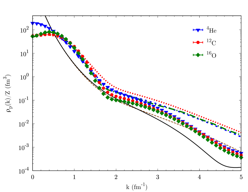
Figure 1: Proton momentum distribution in [4]He, [12]C, and [16]O. Solid symbols are the results for the N²LO $E\tau$ potential with cutoff $R_{0}=1.0\,\rm fm$. Discontinuous lines are the VMC results for [4]He and [12]C Wiringa et al. (2014); Wiringa and cluster VMC results for [16]O Lonardoni et al. (2017) employing the AV18+UIX potential. Dashed brown (solid black) line is the deuteron result for AV18 Wiringa et al. (2014); Wiringa (N²LO with cutoff $R_{0}=1.0\,\rm fm$ Lynn et al. (2017)).

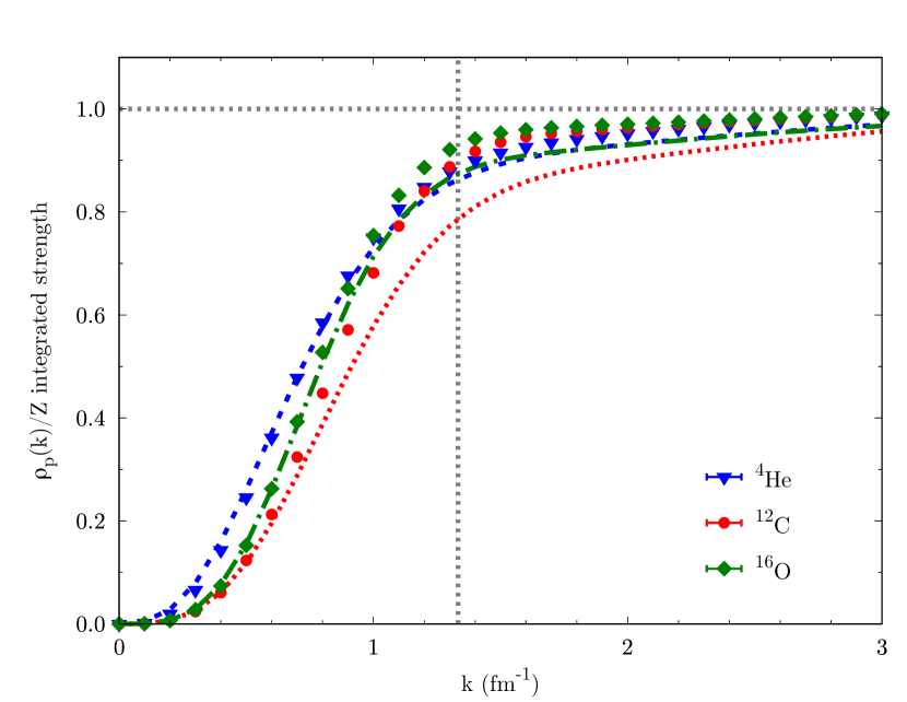
Figure 2: Integrated strength of the proton momentum distributions of Fig. 1 (the same legend is used). The vertical line indicates the Fermi momentum $k_{F}$.

The proton momentum distributions $\rho_{p}(k)$ normalized to the proton number $Z$ for the N²LO $E\tau$ potential with cutoff $R_{0}=1.0\,\rm fm$ are reported in Fig. 1. The VMC and cluster VMC results for the AV18+UIX potential of Refs. Wiringa et al. (2014); Wiringa ; Lonardoni et al. (2017) are also shown for comparison. Up to $\approx 1.0-1.5\,\rm fm^{-1}$, local chiral interactions and phenomenological potentials provide a similar description of the proton momentum distributions. Differences appear at higher momentum, as one would expect being the chiral potentials derived from a low-energy EFT of the nuclear force. This is also evident by looking at Fig. 2, where the integrated strength of the proton momentum distribution is shown as a function of $k$. At low momentum, chiral and phenomenological results are similar for all nuclei. At $2\,\rm fm^{-1}$, most of the strength for chiral interactions is already accounted for: $95.1(1)\%$ in [4]He, $96.3(4)\%$ in [12]C, and $97.0(4)\%$ in [16]O. At $\approx 3.5\,\rm fm^{-1}$ all the strength for chiral interactions is saturated, while phenomenological potentials still contribute until $\approx 4.5-5.0\,\rm fm^{-1}$, as indicated by the higher tail of $\rho_{N}(k)$ at high momentum (Fig. 1). The kinetic energy derived from the single-nucleon momentum distribution,

$$K_{N}=-\frac{\hbar^{2}}{2m}\int\frac{d\mathbf{k}}{(2\pi)^{3}}\,k^{2}\,\rho_{N}(\mathbf{k}),$$ (14)

in general saturates at higher momentum. For both local chiral interactions and phenomenological potentials, $K_{N}$ is consistent with the direct VMC calculation for $k\gtrsim 6\,\rm fm^{-1}$. Local chiral interactions result however in $\approx 20\%$ to $\approx 35\%$ less kinetic energy than the phenomenological counterparts.

It is interesting to observe that at high momentum, the tail of the momentum distribution manifests the expected universal behavior, i.e., the independence of the high-momentum component of $\rho_{N}(k)$ upon the specific nucleus. Such universality has been discussed at length in a number of works (see, for instance, Refs. Feldmeier et al. (2011); Alvioli et al. (2012, 2013, 2016)). We show here (see Fig. 1) that, depending on the choice of the potential, the universal behavior itself is different. This is a consequence of the nature of the high-momentum components of the momentum distribution, which are determined by short-range correlations, i.e., by the short-range structure of the employed Hamiltonian. Local chiral interactions and phenomenological potentials are characterized by different short-range physics, which are reflected in different tails of the momentum distribution.

We show in Fig. 3 the effect of correlations to the proton momentum distribution in [16]O. Blue down triangles refer to the calculation employing the mean-field wave function of Eq. 3. Brown up triangles, red circles, and green diamonds are results for the correlated wave function of Eq. 2 including spin/isospin-independent two-body, full two-body, and two- plus three-body correlations, respectively. Results have been obtained by optimizing the different wave functions so as to obtain the same charge radius reported in Table 1. Similarly to the case of phenomenological potentials Pieper et al. (1992); Alvioli et al. (2005), the mean-field part of the wave function dominates the momentum distribution for $k\lesssim 1.3\,{\rm fm^{-1}}\approx k_{F}$. Correlations are fundamental for the construction of higher-momentum components of $\rho_{N}(k)$, dominated, in particular, by two-body spin/isospin correlations. Three-body correlations have a small effect on the momentum distribution for chiral interactions, enhancing $\rho_{N}(k)$ around $2\,\rm fm^{-1}$ and at higher momentum, $k>4\,\rm fm^{-1}$.

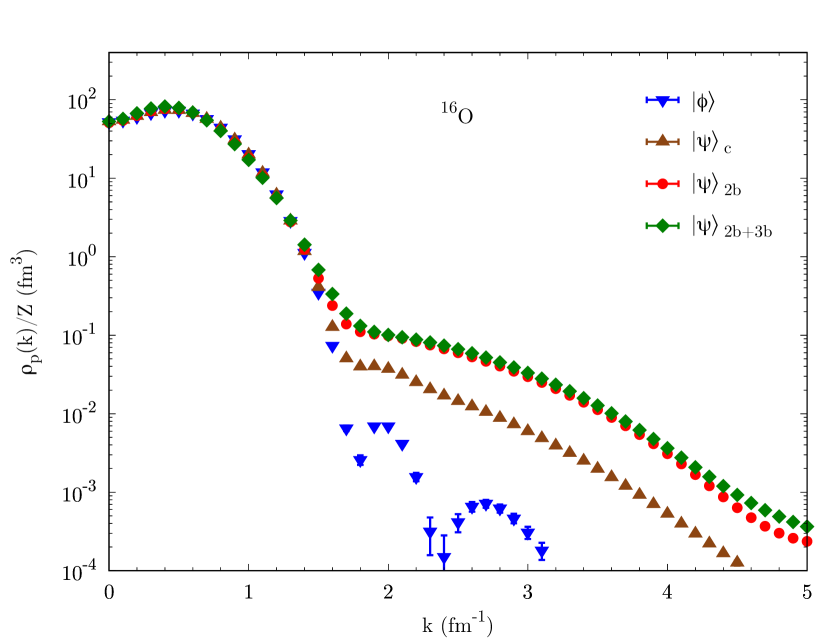
Figure 3: Proton momentum distribution in [16]O. $|\Phi\rangle$ is the result for the mean-field wave function of Eq. 3. $|\Psi\rangle_{\rm c}$, $|\Psi\rangle_{\rm 2b}$, and $|\Psi\rangle_{\rm 2b+3b}$ are the results for the correlated wave function of Eq. 2 employing spin/isospin-independent two-body, full two-body, and two- plus three-body correlations, respectively.

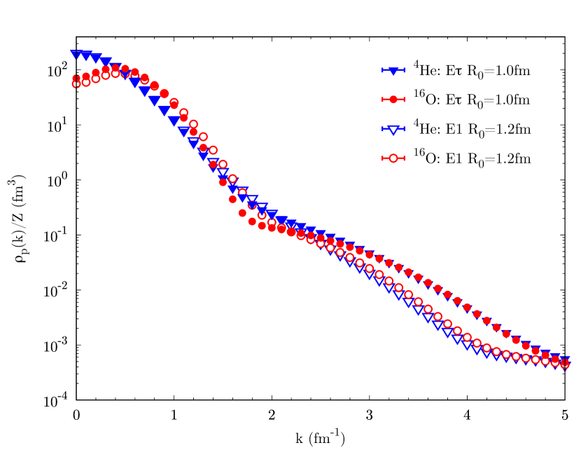
Figure 4: Proton momentum distribution in [4]He and [16]O. Solid symbols are the results for the N²LO $E\tau$ potential with cutoff $R_{0}=1.0\,\rm fm$. Empty symbols are the results for the N²LO $E\mathbbm{1}$ potential with cutoff $R_{0}=1.2\,\rm fm$.

Ground-state properties of light- and medium-mass nuclei, such as binding energies, charge radii, and charge form factors, are independent of the choice of the coordinate-space cutoff for the employed local chiral interactions Lynn et al. (2017); Lonardoni et al. (2018b, a). However, the effect of using softer potentials (larger coordinate-space cutoff) is visible in the momentum distributions, as shown in Fig. 4. For a given system, different interactions provide a similar description of the mean-field part of the momentum distribution ($k\lesssim k_{F}$). Higher momentum components of $\rho_{N}(k)$ are instead reduced for softer potentials. However, as already discussed above, for a given interaction the universality of the high-momentum components of $\rho_{N}(k)$ is preserved.

In [4]He both parametrizations of the three-body force ($E\tau$ and $E\mathbbm{1}$) for a given cutoff provide consistent results for the single-nucleon momentum distribution. The same observation applies to [16]O, for which, however, the $E\tau$ parametrization with cutoff $R_{0}=1.2\,\rm fm$ has not been considered in this work due to the large overbinding predicted by such a potential Lonardoni et al. (2018b, a). Calculations for [12]C have been performed for the $E\tau$ $R_{0}=1.0\,\rm fm$ potential only due to the large computational cost.

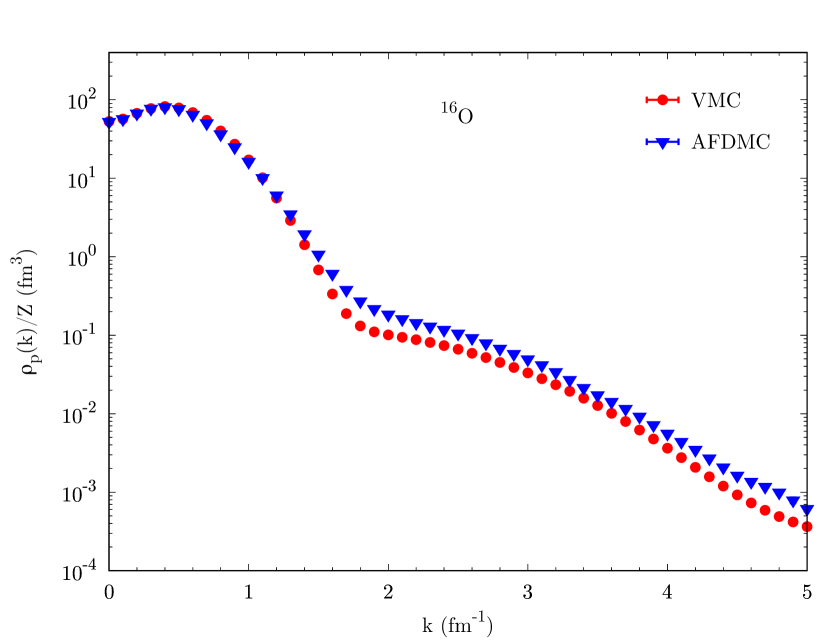
Figure 5: VMC and AFDMC proton momentum distributions in [16]O.

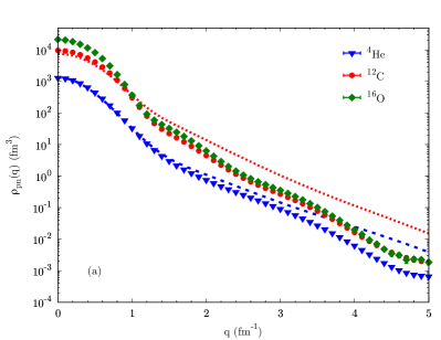
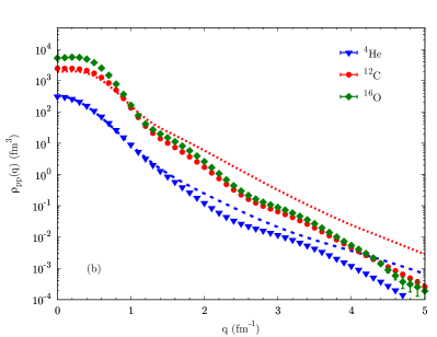
Figure 6: Two-nucleon momentum distributions integrated over $Q$: (a) $pn$ pairs and (b) $pp$ pairs. Solid symbols are the results for the N²LO $E\tau$ potential with cutoff $R_{0}=1.0\,\rm fm$. Lines are VMC results for the AV18+UX potential Wiringa et al. (2014); R. B. Wiringa .

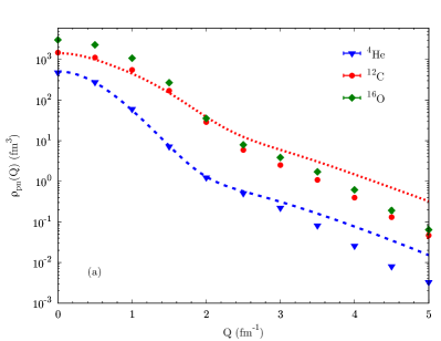
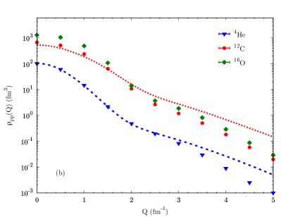
Figure 7: Two-nucleon momentum distributions integrated over $q$: (a) $pn$ pairs and (b) $pp$ pairs. Solid symbols are the results for the N²LO $E\tau$ potential with cutoff $R_{0}=1.0\,\rm fm$. Lines are VMC results for the AV18+UX potential Wiringa et al. (2014); R. B. Wiringa .

Figure 5 shows the VMC and AFDMC results for the proton momentum distribution in [16]O, where the latter are extrapolated from mixed estimates (see Ref. Lonardoni et al. (2018a) for details). The AFDMC results are expected to be more accurate, as they evaluate the expectation values obtained through imaginary time propagation to the ground state. However, the AFDMC calculation for $A=16$ required $\approx 10^{5}$ more computing time than that of the VMC, due to the different scaling of the two Monte Carlo algorithms with the number of particles and the additional statistics required to obtain comparable statistical errors. In [16]O, the AFDMC results are $\approx 35\%$ higher than the VMC in the high-momentum region $(k\gtrsim 2\,\rm fm^{-1})$. Similar results are found for [4]He. Improved trial wave functions, such as those described in Ref. Lonardoni et al. (2018a), could, in principle, bring the VMC results in closer agreement to those of AFDMC. However, the additional required computing time could be prohibitive for larger systems, already at the VMC level. Studies in this direction are in progress.

V Results: two-nucleon momentum distributions

We present in Fig. 6 the two-nucleon momentum distributions as a function of the relative momentum $q$ (the center-of-mass momentum $Q$ is integrated over). Solid symbols are the results for the N²LO $E\tau$ interaction with cutoff $R_{0}=1.0\,\rm fm$. Dotted and dashed lines refer to results employing phenomenological potentials, where available Wiringa et al. (2014); R. B. Wiringa . In Fig. 6blue(a) [Fig. 6blue(b)] the momentum distributions for $pn$ ($pp$) pairs are shown. As for the single-nucleon momentum distributions, up to $k\lesssim k_{F}$ there is little difference in the physical description of $\rho_{N\!N}(q)$ provided by chiral and phenomenological interactions. Higher momentum components of $\rho_{N\!N}(q)$ are instead reduced for local chiral forces, in particular in heavier systems. At $q=2\,\rm fm^{-1}$ $97.3(2)\%$ [$98.6(1)\%$] of the $4\,pn$ ($1\,pp$) pairs are accounted for in [4]He. These percentages are $98.8(7)\%$ [$99.1(3)\%$] for the $36\,pn$ ($15\,pp$) pairs in [12]C and $99.1(8)\%$ [$99.4(4)\%$] for the $64\,pn$ ($28\,pp$) pairs in [16]O.

An alternative way to look at two-nucleon momentum distributions is to integrate Eq. 10 over all $q$, leaving a function $\rho_{N\!N}(Q)$ of the center-of-mass momentum $Q$ only. In Fig. 7 we show $\rho_{N\!N}(Q)$ results for the N²LO $E\tau$ potential with cutoff $R_{0}=1.0\,\rm fm$ (solid symbols) compared to available results for phenomenological potentials (dotted and dashed lines) Wiringa et al. (2014); R. B. Wiringa . As in Fig. 6, Fig. 7blue(a) [Fig. 7blue(b)] reports $pn$ ($pp$) momentum distributions. As already observed in Ref. Wiringa et al. (2014) for lighter nuclei and phenomenological potentials, $\rho_{N\!N}(Q)$ for a given system has a smaller falloff at large momentum compared to $\rho_{N\!N}(q)$. The ratio of $pn$ to $pp$ pair is also subject to a smaller variation over the range of $Q$. The same conclusions hold for local chiral interactions up to [16]O, the results of which are similar to those of phenomenological potentials up to $Q\approx 2\,\rm fm^{-1}$.

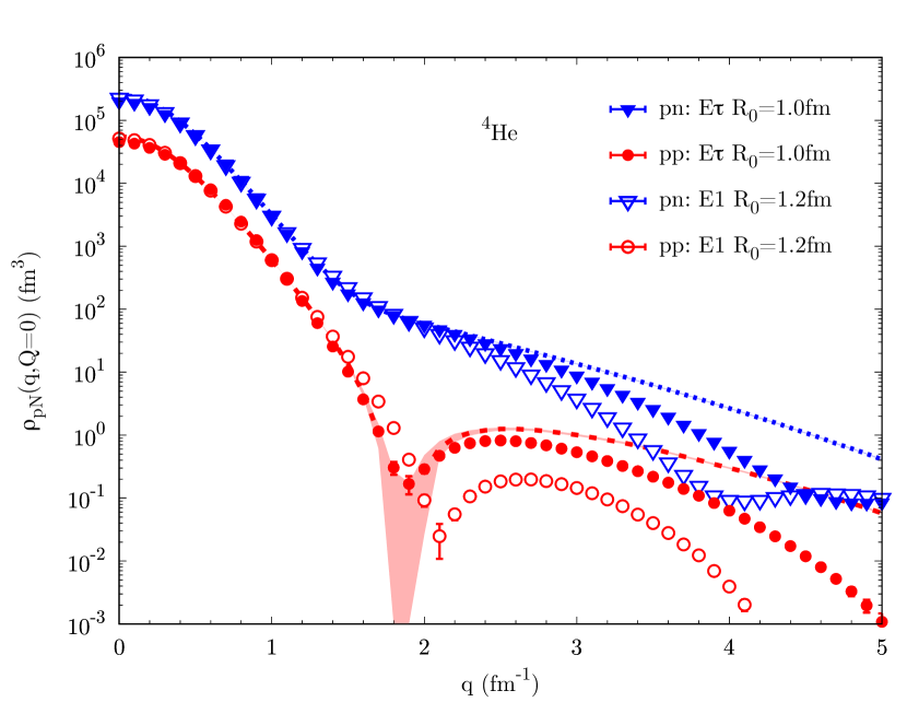
Figure 8: Two-nucleon momentum distributions as a function of $q$ for $Q=0$ in [4]He. Solid symbols are the results for the N²LO $E\tau$ potential with cutoff $R_{0}=1.0\,\rm fm$. Empty symbols are the results for the N²LO $E\mathbbm{1}$ potential with cutoff $R_{0}=1.2\,\rm fm$. Lines with error bands are VMC results for the AV18+UX potential Wiringa et al. (2014); R. B. Wiringa .

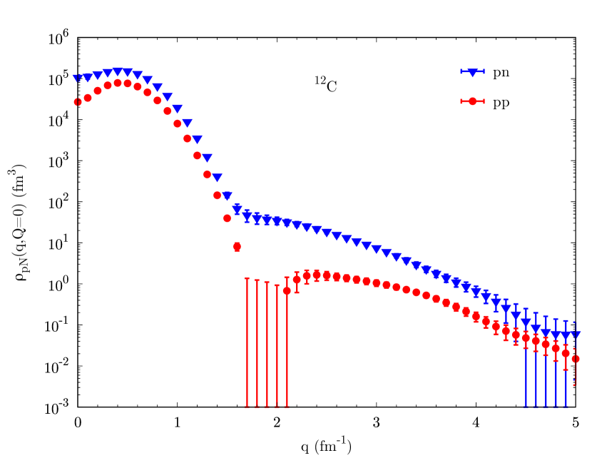
Figure 9: Two-nucleon momentum distributions as a function of $q$ for $Q=0$ in [12]C. The N²LO $E\tau$ potential with cutoff $R_{0}=1.0\,\rm fm$ is used.

The two-nucleon momentum distributions $\rho_{N\!N}(q,Q)$ at $Q=0$ (back-to-back pairs) in [4]He, [12]C, and [16]O are shown in Figs. 8, 9 and 10, respectively. Solid symbols are the results for the N²LO $E\tau$ potential with cutoff $R_{0}=1.0\,\rm fm$. Empty symbols are those for the N²LO $E\mathbbm{1}$ potential with cutoff $R_{0}=1.2\,\rm fm$. Blue triangles (red circles) indicate $pn$ ($pp$) pairs. For $A=4$ the VMC results employing phenomenological potentials Wiringa et al. (2014); R. B. Wiringa are also reported for comparison. For [12]C, results are available for the harder interaction only. In all systems $\rho_{N\!N}(q,Q=0)$ is larger for $pn$ pairs compared to $pp$ pairs, in particular for relative momentum in the range $q\approx 1.5-2.5\,\rm fm^{-1}$. The $pp$ distributions present a node in this region, the position of which sits around $2\,\rm fm^{-1}$ for all the nuclei considered in this work. $pn$ pairs show instead a deuteronlike distribution, with a change of slope around $q=1.5\,\rm fm^{-1}$, as for phenomenological potentials Wiringa et al. (2014); R. B. Wiringa . The ratio of $pn$ to $pp$ pairs in the region $q\approx 1.5-2.5\,\rm fm^{-1}$ is $\gtrsim 20$ in [4]He and $\gtrsim 10$ in [12]C and [16]O. The same conclusion holds for both harder and softer potentials. Although there are differences in the description of the two-nucleon momentum distributions, the $pn$ to $pp$ ratio in the region $q\approx 1.5-2.5\,\rm fm^{-1}$ is nearly independent of the employed local chiral interactions.

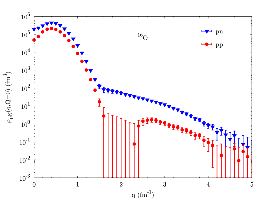
Figure 10: Same as Fig. 9 but for [16]O.

In Fig. 11 we report the ratio between $pp$ and $pn$ pairs as a function of $q$ for back-to-back pairs. The N²LO $E\tau$ potential with cutoff $R_{0}=1.0\,\rm fm$ is used. Results for [4]He employing phenomenological potentials R. B. Wiringa are shown for comparison (solid line). Empty symbols are extracted from experimental data: circles for [4]He from Ref. Korover et al. (2014), squares for [12]C from Ref. Subedi et al. (2008), and diamonds for [27]Al, [56]Fe, and [208]Pb from Ref. Hen et al. (2014). For the employed local chiral interactions all nuclei are consistent with high-momentum data extracted from experiments.

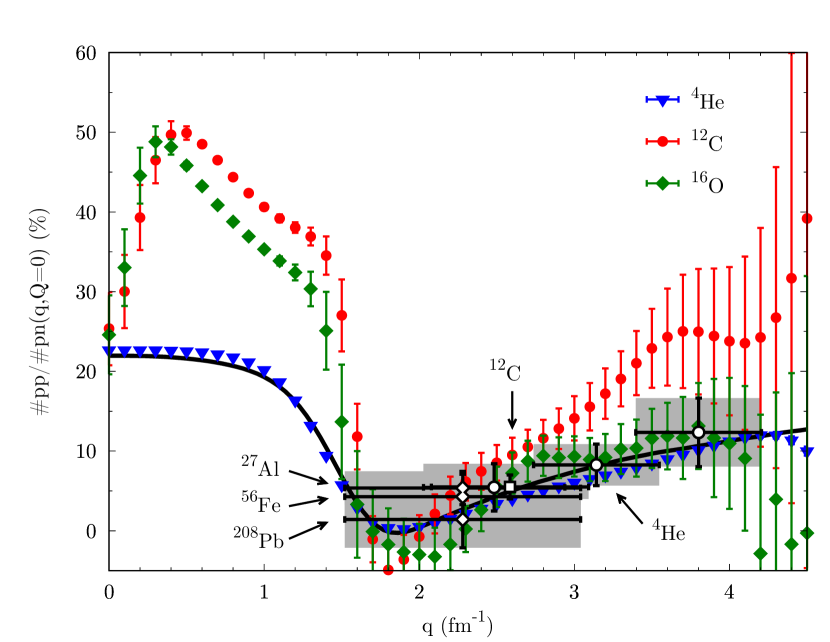
Figure 11: $pp$ pairs to $pn$ pairs ratio as a function of $q$ for $Q=0$. The N²LO $E\tau$ potential with cutoff $R_{0}=1.0\,\rm fm$ is used. The solid curve was extracted from the two-body momentum distributions in [4]He for phenomenological potentials R. B. Wiringa . Black empty symbols and gray bands were extracted from experimental data: [4]He from Ref. Korover et al. (2014), [12]C from Ref. Subedi et al. (2008), and [27]Al, [56]Fe, and [208]Pb from Ref. Hen et al. (2014).

Note that the wave function of Eq. 2 only includes linear spin/isospin-dependent two-body correlations; i.e., only one nucleon pair is correlated at a time. Improved two-body correlations (see Ref. Lonardoni et al. (2018a) for details) are under study, but the increased computing time requested to evaluate the full wave function will make the calculation of two-body momentum distributions for medium-mass nuclei computationally challenging. However, preliminary tests in [4]He show an $\approx 8-18\%$ variation of the $pp$ to $pn$ ratio in the range $q\approx 2.5-4.0\,\rm fm^{-1}$, result still compatible with the available data extracted from experiments.

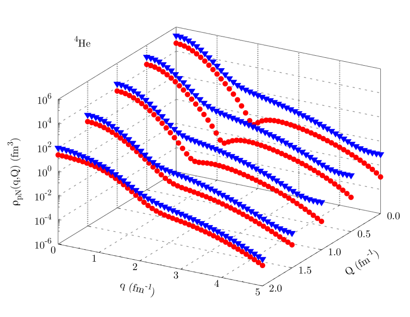
Figure 12: Two-nucleon momentum distributions in [4]He for the N²LO $E\tau$ potential with cutoff $R_{0}=1.0\,\rm fm$. Blue triangles refer to $pn$ pairs, and red circles refer to $pp$ pairs.

The electron scattering experiments necessarily involve two-nucleon currents, which are not included in this work. Here we provide comparisons to other calculations of single- and two-nucleon momentum distributions Alvioli et al. (2013); Wiringa et al. (2014); Alvioli et al. (2016); Lonardoni et al. (2017). These currents provide a $30-40\%$ constructive interference in the inclusive transverse quasielastic electron scattering Lovato et al. (2016) and in the axial response relevant to neutrino scattering Lovato et al. (2018). It remains to be investigated how they impact the back-to-back exclusive measurements.

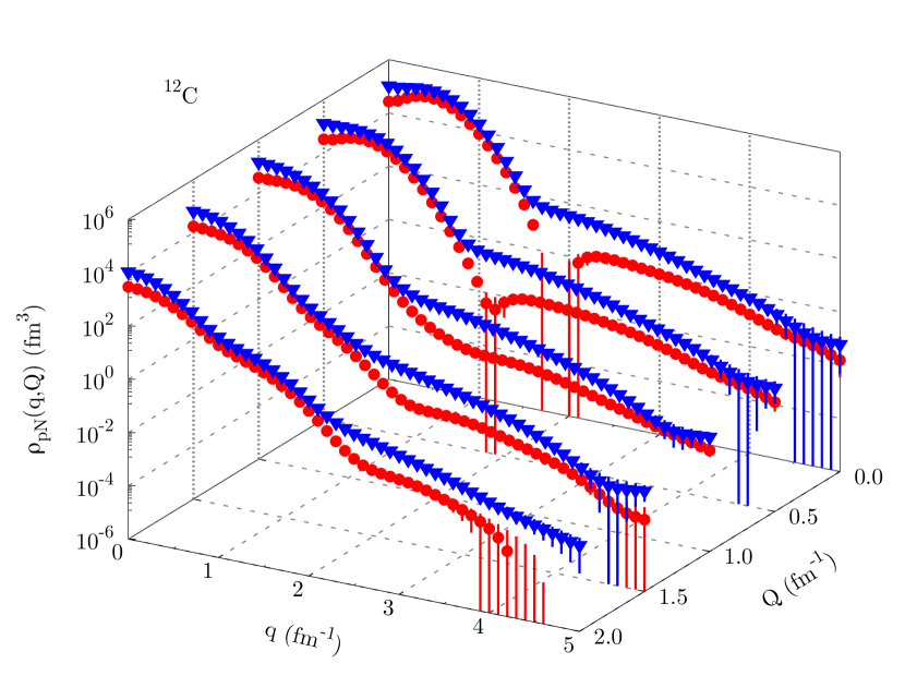
Figure 13: Same as Fig. 12 but for [12]C.

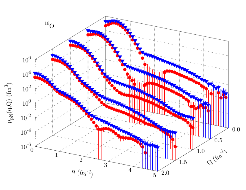
Figure 14: Same as Fig. 12 but for [16]O.

Finally, the evolution of the two-nucleon momentum distribution as a function of $Q$ is shown in Figs. 12, 13 and 14 for [4]He, [12]C, and [16]O, respectively. As in the previous plots, blue triangles (red circles) are the results for $pn$ ($pp$) pairs employing the N²LO $E\tau$ potential with cutoff $R_{0}=1.0\,\rm fm$. The description of $\rho_{pn}(q,Q)$ and $\rho_{pp}(q,Q)$ in [4]He as $Q$ increases is analogous to that provided by phenomenological potentials Wiringa et al. (2014); R. B. Wiringa . The node in the $pp$ distribution gradually disappears, while the deuteronlike distribution of $pn$ pairs is maintained up to large $Q$. The same physical picture holds for larger nuclei up to $A=16$. For $Q\gtrsim 1.5\,\rm fm^{-1}$ the node in the $pp$ momentum distributions is completely filled in, and the $pn$ to $pp$ ratio is largely reduced.

The tables of single- and two-nucleon momentum distributions in [4]He, [12]C, and [16]O for local chiral potentials are available as Supplemental Material sup and as part of the online quantum Monte Carlo momentum distribution collection Wiringa ; R. B. Wiringa .

VI Summary

We presented VMC calculations of the single- and two-nucleon momentum distributions in [4]He, [12]C, and [16]O employing local chiral interactions at N²LO. The description of the momentum distributions at low and moderate momenta up to $\approx 2k_{F}$ is similar to that provided by phenomenological potentials at low momentum, while higher-momentum components are typically reduced, consistent with the lower-energy regime of chiral EFT interactions.

The effect of short-range correlations on the high-momentum components of the single-nucleon momentum distribution is found to be large and dominant also for local chiral interactions. The universality of the tail of the momentum distribution is confirmed, but only within the same family of interactions.

The two-nucleon momentum distributions as a function of the relative momentum $q$ of the nucleon pair, of the center-of-mass momentum $Q$ of the pair, and of both $q$ and $Q$ are shown. The results for back-to-back pairs confirm the large $pn$ to $pp$ pairs ratio in the regime $q\approx 1.5-2.5\,\rm fm^{-1}$ up to [16]O, which appears to be independent of the employed interaction scheme. The $pp$ to $pn$ ratio for local chiral interactions is compatible with available experimental data extracted from electron scattering experiments in the range $q\approx 2.5-4.0\,\rm fm^{-1}$ up to $A=16$.

It will be interesting to analyze the results of this work using factorized asymptotic wave functions and the short-range correlations as done in Ref. Weiss et al. (2018) for phenomenological potentials. This will provide information about how sensitive are the contacts and ratios of contacts to the scale and scheme of the calculations, opening the possibility of relating a very large class of observables to ground-state calculations.