Capacity of Multiple One-Bit Transceivers in a Rayleigh Environment

Abstract

We analyze the channel capacity of a system with a large number of one-bit transceivers in a classical Rayleigh environment with perfect channel information at the receiver. With $M$ transmitters and $N=\alpha M$ receivers, we derive an expression of the capacity per transmitter $\mathcal{C}$, where $\mathcal{C}\leq\min(1,\alpha)$, as a function of $\alpha$ and signal-to-noise ratio (SNR) $\rho$, when $M\to\infty$. We show that our expression is a good approximation for small $M$, and provide simple approximations of $\mathcal{C}$ for various ranges of $\alpha$ and $\rho$. We conclude that at high ${\rm SNR}$, $\mathcal{C}$ reaches its upper limit of one only if $\alpha>1.24$. Expressions for determining when $\mathcal{C}$ “saturates” as a function of $\alpha$ and $\rho$ are given.

I Introduction

In an effort to save power and cost in wideband wireless transceiver systems, low-resolution (especially one-bit) analog-to-digital converters (ADCs) [1, 2, 3, 4, 5, 6, 7, 8, 9, 10, 11, 12, 13] and digital-to-analog converters (DACs) [14, 15, 16] are being considered in transmitter and receiver chains, especially in systems involving many such chains. The nonlinearity introduced by coarse quantization becomes a limiting factor in the achievable throughput of such a wireless system. Channel capacity is one measure of this throughput.

There is a rich literature on the subject of capacity with coarse quantization. The capacity of a system with one-bit ADCs at the receiver is analyzed in [1, 2, 3, 4, 6, 7, 5, 8, 9] with various assumptions about the channel, the channel information, and communication schemes. Communication techniques including channel estimation and signal detection for a multiple-input multiple-output (MIMO) system with one-bit ADCs at the receiver are studied in [10, 11, 12, 13]. A communication system with one-bit DACs at the transmitter is studied in [14, 15, 16].

While many of the efforts consider low-resolution quantization effects at the transmitter or receiver, a few consider low-resolution quantization on both, including [17] and [18]. A linear minimum-mean-squared-error precoder design is proposed for a downlink massive MIMO scenario to mitigate the quantization distortion in [17] and the performance analysis of a system with a small number of one-bit transceivers is studied in [18]. We focus on a model where one-bit quantization is considered at both the transmitter and receiver:

$${\mathbf{y}}=\text{sign}\left(\sqrt{\frac{\rho}{M}}H{\mathbf{x}}+{\mathbf{v}}\right),{\mathbf{x}}\in\{\pm 1\}^{M},$$ (1)

where $M$ and $N$ are the number of transmitters and receivers, ${\mathbf{x}}\in\{\pm 1\}^{M}$ and ${\mathbf{y}}\in\{\pm 1\}^{N}$ are the transmitted and received signals, $H\in\mathbb{R}^{N\times M}$ is the channel matrix known to the receiver, ${\mathbf{v}}\in\mathbb{R}^{N}$ is the additive Gaussian noise with ${\mathbf{v}}\sim\mathcal{N}(0,I)$ and ${\mathbf{v}}$ is independent of ${\mathbf{x}}$ and $H$, $\rho$ is the expected received SNR at each receive antenna. The function $\text{sign}(\cdot)$ provides the sign of the input as its output. The channel is modeled as real-valued since only the in-phase (I) information is used and the quadrature (Q) phase is ignored at the receiver. A Rayleigh channel is assumed, with each element to be independent Gaussian $\mathcal{N}(0,1)$. This assumption appears to hold for non-line of sight (NLOS) channels in many frequency bands [19], and also appears in the analysis in [6, 7, 8, 9, 10, 11, 14].

Our contribution is a large $M$ and $N$ analysis, where the ratio $\alpha=\frac{N}{M}$ is constant, of the capacity for the model (1). Analytical expressions are derived that can be used to explain the behavior of the system in various limiting regimes of operation in $\alpha$ and ${\rm SNR}$.

II Capacity for a large number of transmitters and receivers

The capacity of the channel in (1) as a function of $\rho$, $M$, and $N$ is

$$C(\rho,M,N)=\frac{1}{M}\max\limits_{p_{\rm x}(\cdot),{\mathbf{x}}\in\{\pm 1\}^{M}}{\mathbf{I}}({\mathbf{x}};{\mathbf{y}},H),$$ (2)

where we have normalized by $M$, and where $p_{\rm x}(\cdot)$ is the input distribution independent of $H$, and ${\mathbf{I}}(\cdot;\cdot)$ is the mutual information notation. When $M,N\to\infty$ with a ratio $\alpha=\frac{N}{M}$, the capacity $\mathcal{C}$ is defined as

$$\mathcal{C}(\rho,\alpha)=\lim_{M\to\infty}C(\rho,M,\alpha M).$$ (3)

We can readily see that $C(\rho,M,N)\leq\min(1,\alpha)$ because each transmitter can transmit at most one bit of information, and each receiver can decode at most one bit of information. Therefore, $\mathcal{C}(\rho,\alpha)\leq\min(1,\alpha)$ for all $\alpha$ and $\rho$.

Limiting capacities such as (3) are difficult to compute in closed form, but the “replica method” [20] can be brought to bear on the problem. Some details of how to apply the method are presented in Section IV. For now, we present the result:

$$\mathcal{C}(\rho,\alpha)=\min\Big{(}\alpha(c(\rho)-c(A^{2}q))+\frac{1}{2\ln 2}(E+Eq)$$

$$-\frac{1}{\sqrt{2\pi}}\int_{\mathbb{R}}\log_{2}(\cosh(E+\sqrt{E}z))e^{-z^{2}/2}dz,1\Big{)},$$ (4)

where $c(\rho)$ is the capacity of a single transceiver with SNR $\rho$, which is defined as

$$c(\rho)=1-\mathbb{E}_{z}\left(\mathcal{H}_{2}(Q(\sqrt{\rho}z))\right),z\sim\mathcal{N}(0,1),$$ (5)

where $\mathcal{H}_{2}(p)=-(p\log_{2}p+(1-p)\log_{2}(1-p))$ is the binary entropy function, and $q,E,A$ are the solutions of

$$q=\frac{1}{\sqrt{2\pi}}\int_{\mathbb{R}}\tanh(\sqrt{E}z+E)e^{-z^{2}/2}dz,$$ (6)

$$E=\frac{\alpha A^{2}}{\pi\sqrt{2\pi}}\int_{\mathbb{R}}\frac{\exp\left(-(A^{2}q+\frac{1}{2})z^{2}\right)}{Q(A\sqrt{q}z)}dz,$$ (7)

$$A=\sqrt{\frac{\rho}{1+\rho(1-q)}}.$$ (8)

Equation (4) gives the capacity for any SNR $\rho$ and $\alpha$, and some limiting situations are readily analyzed, including: (i) high SNR, $\rho\to\infty$; (ii) low SNR, $\rho\to 0$; (iii) many more receivers than transmitters, $\alpha\to\infty$; (iv) many more transmitters than receivers, $\alpha\to 0$. These are now presented, with only limited proofs.

II-A High SNR ($\rho\to\infty$)

When $\rho\to\infty$, the system is effectively becoming “noise-free”, and we might expect $\mathcal{C}\to 1$, but as we show this does not happen for all $\alpha$. For ${\rm SNR}\to\infty$, $A=\sqrt{\frac{1}{1-q}}$, and (4) becomes

$$\mathcal{C}(\alpha,\rho)=\min\Big{(}\alpha\big{(}1-c(\frac{q}{1-q})\big{)}+\frac{1}{2\ln 2}(E+Eq)$$

$$-\frac{1}{\sqrt{2\pi}}\int_{\mathbb{R}}\log_{2}(\cosh(E+\sqrt{E}z))e^{-z^{2}/2}dz,1\Big{)},$$ (9)

where $c(\cdot)$ is defined in (5), (7) can be simplified as

$$E=\frac{\alpha}{\pi\sqrt{2\pi(1-q)}}\int_{\mathbb{R}}\frac{\exp(-(q+\frac{1}{2})z^{2})}{Q(\sqrt{q}z)}dz,$$ (10)

and $E,q$ are the solution of (6) and (10).

The expression (9) is not especially intuitive, but it is not difficult to solve. We show some numerical examples in Section III. It turns out that in this case, solving (9) is essentially equivalent to solving for the “quenched entropy” for Gibbs learning of the Ising perceptron (Section 7.2 in [21]).

II-B Low SNR ($\rho\to 0$)

When $\rho\to 0$, (6), (7), and (8) become

$$q\to\frac{2\alpha\rho}{\pi},\;E\to\frac{2\alpha\rho}{\pi},\;A\to\sqrt{\rho}.$$ (11)

For small $x$, we use a Taylor series expansion to obtain

$$Q(x) \ln(Q(x))=-\frac{\ln 2}{2}-\frac{(1-\ln 2)x}{\sqrt{2\pi}}+\frac{x^{2}}{2\pi}$$

$$+\frac{(1-\ln 2)\pi+2\sqrt{2\pi}}{6\pi\sqrt{2\pi}}x^{3}+\frac{\pi-1}{6\pi^{2}}x^{4}+o(x^{4}),$$

$$\ln (\cosh(x))=\frac{x^{2}}{2}-\frac{x^{4}}{12}+o(x^{4}).$$

Then

$$\mathcal{C}(\rho,\alpha)\approx\frac{\alpha\rho}{\pi\ln 2}-\frac{\alpha^{2}+(\pi-1)\alpha}{\pi^{2}\ln 2}\rho^{2},$$ (12)

to second order in $\rho$. It turns out that this result matches the expression in [6], with a difference in factor of $\frac{1}{2\ln 2}$ that comes from the fact that [6] considers two bits per transmission, and ‘nats’ instead of ‘bits’.

II-C $N>>M$ ($\alpha\to\infty$)

When $\alpha\to\infty$, (6)-(8) becomes

$$q\to 1,A\to\sqrt{\rho},$$

$$E\to\frac{\alpha\rho}{\pi\sqrt{2\pi}}\int_{\mathbb{R}}\frac{\exp\left(-(\rho+\frac{1}{2})z^{2}\right)}{Q(\sqrt{\rho}z)}dz.$$ (13)

and

$$\mathcal{C}(\rho,\alpha)\approx\min\Big{(}1,\frac{E}{\ln 2}-$$

$$\int_{\mathbb{R}}\frac{1}{\sqrt{2\pi}}e^{-z^{2}/2}\log_{2}(\cosh(E+\sqrt{E}z))dz\Big{)},$$ (14)

More will be said about this in Section III.

II-D $N<<M$ ($\alpha\to 0$)

When $\alpha\to 0$, the first order approximations of $q$ and $E$ based on (6)-(8) become

$$q=\frac{2\rho\alpha}{(1+\rho)\pi}+o(\alpha),E=\frac{2\rho\alpha}{(1+\rho)\pi}+o(\alpha).$$ (15)

Therefore,

$$\mathcal{C}(\rho,\alpha)\approx c(\rho)\alpha-\frac{\rho^{2}}{\pi^{2}(1+\rho)^{2}\ln 2}\alpha^{2},$$ (16)

where $c(\rho)$ is the capacity of a single transceiver, defined in (5).

III numerical evaluation of capacity

We first compare $C(\rho,M,\alpha M)$ in (2) with $\mathcal{C}(\rho,\alpha)$ in (4) for $M=8$ and $\alpha\in\{0.25,\cdots,1.75\}$, to show how the large-$M$ and $N$ limit (4) can be used to approximate the exact capacity. Figure 1 displays that the approximation is accurate for small $M$ for a wide range of SNR (from 0 dB to 30 dB) when $\mathcal{C}(\rho,\alpha)\leq 0.7$. When $\mathcal{C}(\rho,\alpha)$ is larger than 0.7, $M=8$ is not big enough and a larger $M$ is required to get a valid approximation. We can see that $\mathcal{C}(\rho,\alpha)$ can saturate at 1 when $\alpha\geq 1.5$ with SNR smaller than 30 dB, and an SNR higher than 30 dB is required to achieve the maximum for $\alpha=1.25$, but $\mathcal{C}(\rho,\alpha)$ cannot achieve the maximum when $\alpha\leq 1$. We will show later that $\alpha>1.24$ is required to achieve the maximum.

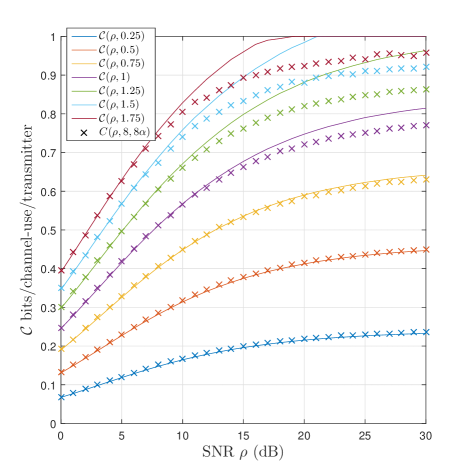
Figure 1: Comparison between $C(\rho,M,\alpha M)$ (2) and $\mathcal{C}(\rho,\alpha)$ (4) with $M=8$ for $\alpha\in\{0.25,\cdots,1.75\}$ with SNR varying from 0 dB to 30 dB. The accuracy of the approximation in a wide range of SNR shows that $M=8$ is big enough to get a valid approximation with $\mathcal{C}(\rho,\alpha)\leq 0.7$.

Figure 2 displays $\mathcal{C}(\rho,\alpha)$ in (4) for $\alpha$ and $\rho$ varying from 0.1 to 10 with step 0.1. We can see that $\mathcal{C}(\rho,\alpha)$ increases linearly with $\rho$ and $\alpha$ when $\rho$ and $\alpha$ are small, and the rate of increase slows down dramatically as $\rho$ and $\alpha$ grow and $\mathcal{C}$ nears saturation at $\mathcal{C}\approx 1$. When $\alpha$ is small but $\rho$ is large, $\mathcal{C}(\rho,\alpha)$ saturates at $\mathcal{C}(\rho,\alpha)\approx\alpha$ (its upper bound). When $\rho$ is small but $\alpha$ is large, we can see that $\mathcal{C}(\rho,\alpha)$ increases with $\alpha$ and reaches its maximum value 1. We show that for any $\rho$, $\mathcal{C}(\rho,\alpha)\to 1$ when $\alpha\to\infty$.

Contours of constant $\mathcal{C}(\rho,\alpha)$ for $\rho\leq 4$ and $\alpha\leq 4$ are shown in Figure 3. We can observe that there is generally a sharp tradeoff between $\rho$ and $\alpha$, and that operating near the knee in the curve is generally desirable for a given capacity since both $\alpha$ and $\rho$ are small.

Furthermore, the contours are dense when $\mathcal{C}(\rho,\alpha)\leq 0.8$ and start becoming sparse when $\mathcal{C}(\rho,\alpha)\geq 0.8$, thus showing that $\mathcal{C}(\rho,\alpha)$ has started to “saturate” at 0.8 and improves only slowly with further increases in either $\alpha$ or $\rho$.

The contours allow us to explore optimal operating points. For example, given a cost function where $\alpha+\rho=d$ for some constant $d$, we find an approximately optimal point to achieve $\mathcal{C}(\rho,\alpha)=0.8$ is $\alpha=3.4$ and $\rho\approx 2.07$. Attempts to make $\alpha$ smaller will require significant increase in $\rho$, and attempts to make $\rho$ smaller will require significant increase in $\alpha$.

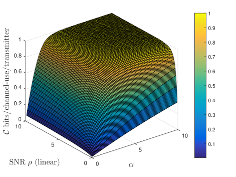
Figure 2: $\mathcal{C}(\rho,\alpha)$ (4) versus $\rho$ and $\alpha$ with $0.1\leq\rho\leq 10$ and $0.1\leq\alpha\leq 10$. $\mathcal{C}(\rho,\alpha)$ increases linearly with $\rho$ and $\alpha$ when $\rho$ and $\alpha$ are small but $\mathcal{C}(\rho,\alpha)$ “saturates” quickly.

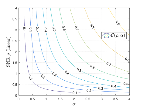
Figure 3: Contour plot of $\mathcal{C}(\rho,\alpha)$ (4) with $\alpha\leq 4$ and $\rho\leq 4$. The gap between the adjacent contours becomes large as $\mathcal{C}(\rho,\alpha)$ increases, which shows the increasing demands on $\rho$ and $\alpha$ to increase $\mathcal{C}(\rho,\alpha)$.

Figure 4 shows the accuracy of the approximations of $\mathcal{C}(\rho,\alpha)$ at high and low SNR. Plotted are examples when SNR is large (10 dB to 30 dB) and SNR is low (-10 dB, $\rho=0.1$) of the actual capacity (4) and the corresponding approximations (9) and (12). Of particular interest is the approximately linear growth in (9) with $\alpha$ until it reaches the $\mathcal{C}=1$ saturation point when $\alpha\approx 1.24$. This hard limit value of 1.24 receive antennas for every transmit antenna is perhaps surprising.

The curves for low SNR show that $\mathcal{C}(\rho,\alpha)$ at $\rho=0.1$ is close to the low SNR approximation in (12) with a simple second order expression when $\alpha\leq 4$. In general, when $\rho\leq 0.1$, we need $\alpha\leq 0.4/\rho$ for an accurate low SNR approximation according to (11).

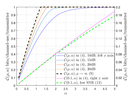
Figure 4: Comparison between $\mathcal{C}(\rho,\alpha)$ (4) at high SNR (10 dB to 30 dB), low SNR (-10 dB, $\rho=0.1$), and their corresponding approximations in (9) and (12). The curve at $\rho=10$ (10 dB) is already close to the noise-free case, which increases nearly linearly with $\alpha$ before saturation at $\alpha\approx 1.24$. The low SNR approximation (12) is similarly accurate when $\rho=0.1$ for $\alpha\leq 4$. In general, we need $\alpha\leq 0.4/\rho$ for an accurate low SNR approximation when $\rho\leq 0.1$.

Figure 5 presents a comparison of (4) with the large $\alpha$, small $\alpha$ approximations in (14) and (16). We obtain excellent agreement for even the modest values $\alpha=5$ and $\alpha=1$ over a wide range of SNR. Moreover, according to (13), when $\alpha\to\infty$, we have $E\to\infty$ for any $\rho>0$, and thus $\mathcal{C}(\rho,\alpha)\to 1$. This differs from the high SNR case, where $\mathcal{C}(\rho,\alpha)<1$ when $\alpha<1.24$ even as $\rho\to\infty$.

III-A Tradeoff between $\alpha$ and $\rho$ for fixed $\mathcal{C}$

We are interested in characterizing the contours in Figure 3 analytically, and we use the large $\alpha$ approximation for $\mathcal{C}$ in (14). Since $\mathcal{C}$ in (14) is just a function of $E$, to achieve some target capacity $\mathcal{C}$, we solve for $E$ numerically, and denote the result as $E_{\mathcal{C}}$. With $E=E_{\mathcal{C}}$, (13) then provides the relationship between $\alpha$ and $\rho$. To simplify the relationship, (13) can be further approximated as

$$E_{\mathcal{C}}\approx\frac{\alpha}{\pi}(-0.3\rho^{2}+1.8\rho)$$ (17)

with good accuracy when $\rho\leq 1.5$. The relationship between $\alpha$ and $\rho$ is then

$$\rho\approx 3-\sqrt{9-\frac{10E_{\mathcal{C}}\pi}{3\alpha}}.$$ (18)

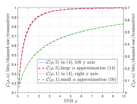
Figure 5: The comparison between the capacity $\mathcal{C}(\rho,\alpha)$ (4) with large $\alpha$ ($\alpha=5$), small $\alpha$ ($\alpha=1$) and their corresponding approximations in (14) and (16). The good approximations over a wide range of SNR shows that $\alpha=5$ is big enough and $\alpha=1$ is small enough to use (14) and (16) for accurate approximations.

To verify the approximation in (18), we compare the actual SNR $\rho$ with the approximated $\rho$ (18) in Figure 6. Shown are contours for $\mathcal{C}=0.6,\ldots,0.9$ and $\alpha\in[5,10]$. The solid lines are the contour plot of $\mathcal{C}(\rho,\alpha)$ (4), and the dashed lines are (18). We see good agreement over a wide range of $\alpha$.

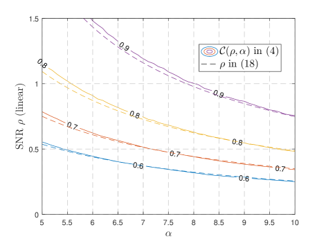
Figure 6: Comparison between the actual SNR $\rho$ and the approximated SNR (18) for the contours $\mathcal{C}=0.6,\ldots,0.9$. The solid lines are contour plots of (4), and the dashed lines present the approximation of $\rho$ (18) as a function of $\alpha$.

Clearly, there are many other comparisons and tradeoffs we can analyze using (4) and its approximations. We briefly describe how the replica method was applied to obtain (4).

IV Replica Analysis

The replica method, a tool used in statistical mechanics and applied to the theory of spin glass [20], has been applied in many communication system contexts [22, 23, 24, 25, 26], neural networks [27, 21], error-correcting codes [28], and image restoration [29]. A mathematically rigorous justification of the replica method is elusive, but the success of the method maintains its popularity. We apply the method to solve for a closed-form answer to (3). We omit many details, and present only the primary steps.

Because the channel is unknown to the transmitter, according to [18], the optimal input distribution is $p_{x}({\mathbf{x}})=\frac{1}{2^{M}}$, and then (2) becomes

$$C(\rho,M,N) =\frac{1}{M}\left({\mathbf{H}}({\mathbf{y}}|H)-{\mathbf{H}}({\mathbf{y}}|{\mathbf{x}},H)\right),p_{x}({\mathbf{x}})=\frac{1}{2^{M}},$$

where ${\mathbf{H}}(\cdot)$ is the standard definition of entropy.

Since the elements in $H$ are i.i.d. $\mathcal{N}(0,1)$, and ${\mathbf{x}}\in\{\pm 1\}^{M}$, we have $\sqrt{\frac{\rho}{M}}H{\mathbf{x}}\sim\mathcal{N}(0,\rho I)$, and

$${\mathbf{H}}({\mathbf{y}}|{\mathbf{x}},H)=N(1-c(\rho)),$$ (19)

where $c(\rho)$ is defined in (5).

Then, (3) becomes

$$\mathcal{C}(\rho,\alpha)=\lim_{M\to\infty}\frac{{\mathbf{H}}({\mathbf{y}}|H)}{M}-\alpha(1-c(\rho)).$$ (20)

The replica method is used to compute the limit, and the processes are similar to that used in [22, 23, 24, 25, 26].

We start with the identity

$${\mathbf{H}}({\mathbf{y}}|H)=-\frac{1}{\ln 2}\lim_{n\to 0}\frac{\partial}{\partial n}\ln\mathbb{E}_{H,{\mathbf{y}}}(p({\mathbf{y}}|H))^{n},$$

which holds for $n\in\mathbb{R}$. The idea of the replica method is to compute $\mathbb{E}_{H,{\mathbf{y}}}(p({\mathbf{y}}|H))^{n}$ as a function of $n$ by treating $n$ as a positive integer, and then assume the result to be valid for $n\in\mathbb{R}$.

We assume the limit of $M$ and $n$ can commute, then

$$\underset{M\to\infty}{\lim}\frac{{\mathbf{H}}({\mathbf{y}}|H)}{M}=-\frac{1}{\ln 2}\lim_{n\to 0}\frac{\partial}{\partial n}\lim_{M\to\infty}\frac{\ln\Xi_{n}}{M},$$ (21)

where $\Xi_{n}=\mathbb{E}_{H,{\mathbf{y}}}(p({\mathbf{y}}|H))^{n}$.

Now, we regard $n$ as a positive integer and we have

$$\Xi_{n} =\mathbb{E}_{H,{\mathbf{y}}}(p({\mathbf{y}}|H))^{n}=\mathbb{E}_{H}\sum_{{\mathbf{y}}}\left(\prod_{a=0}^{n}\mathbb{E}_{{\mathbf{x}}_{a}}p({\mathbf{y}}|H,{\mathbf{x}}_{a})\right),$$

where ${\mathbf{x}}_{a}$ is the $a$th replica of ${\mathbf{x}}$ ($0\leq a\leq n$), and ${\mathbf{x}}_{a}$ are i.i.d. uniform distributed in $\{\pm 1\}^{M}$.

Based on (1), we further have

$$\Xi_{n} =\mathbb{E}_{{\mathbf{x}}_{0},\cdots,{\mathbf{x}}_{n}}\sum_{{\mathbf{y}}}\mathbb{E}_{H}\left(\prod_{a=0}^{n}\prod_{k=1}^{{N}}Q\left(-y_{k}\sqrt{\frac{\rho}{M}}{\mathbf{h}}_{k}^{T}{\mathbf{x}}_{a}\right)\right)$$

$$=\mathbb{E}_{{\mathbf{x}}_{0},\cdots,{\mathbf{x}}_{n}}[e^{N\mathcal{G}}],$$ (22)

where $y_{k}$ is the $k$th element of ${\mathbf{y}}$, $Q(\cdot)$ is the well-known Q-function, and ${\mathbf{h}}_{k}^{T}$ is the $k$th row of $H$,

$$e^{\mathcal{G}}=\sum_{y}\mathbb{E}_{{\mathbf{h}}}\prod_{a=0}^{n}Q\left(-y\sqrt{\frac{\rho}{M}}{\mathbf{h}}^{T}{\mathbf{x}}_{a}\right)$$ (23)

with $y\in\{\pm 1\},{\mathbf{h}}\sim\mathcal{N}(0,I)$.

Let $u_{a}=\frac{1}{M}{\mathbf{h}}^{T}{\mathbf{x}}_{a}$ and ${\mathbf{u}}=[u_{0},\cdots,u_{n}]^{T}$. Then ${\mathbf{u}}\sim\mathcal{N}(0,R)$, where $R$ is the covariance matrix with elements $R_{ab}=\mathbb{E}(u_{a}u_{b})=\frac{{\mathbf{x}}_{a}^{T}{\mathbf{x}}_{b}}{M}\in[-1,1]$ for $0\leq a<b\leq n$ and $R_{aa}=1$. Then $\mathcal{G}$ only depends on $R$:

$$\mathcal{G}(R)=\ln\left(\sum_{y}\mathbb{E}_{{\mathbf{u}}}\prod_{a=0}^{n}Q\left(-y\sqrt{\rho}u_{a}\right)\right),$$ (24)

and (22) becomes

$$\Xi_{n}=\int_{\mathbb{R}}\cdots\int_{\mathbb{R}}\prod_{a<b}dR_{ab}\mu_{M}(R)e^{N\mathcal{G}(R)},$$

where

$$\mu_{M}(R)=\mathbb{E}_{{\mathbf{x}}_{0},\cdots,{\mathbf{x}}_{n}}\left(\prod_{a<b}\delta(\frac{{\mathbf{x}}_{a}^{T}{\mathbf{x}}_{b}}{M}-R_{ab})\right).$$ (25)

We can consider $\mu_{M}(R)$ as the distribution of a random symmetric matrix ${\mathbf{R}}$, and we have

$$\Xi_{n}=\mathbb{E}_{{\mathbf{R}}}\Big{[}e^{N\mathcal{G}({\mathbf{R}})}\Big{]},{\mathbf{R}}\sim\mu_{M}(R)$$

Similarly to [24], we apply Varadhan’s theorem and Gartner-Ellis theorem[30] and obtain

$$\lim_{M\to\infty}\frac{\ln\Xi_{n}}{M}=\sup_{R}\inf_{\tilde{R}}\underbrace{\left[\alpha\mathcal{G}(R)-\sum_{a<b}\tilde{R}_{ab}R_{ab}+\Lambda(\tilde{R})\right]}_{f(R,\tilde{R})},$$ (26)

where $\tilde{R}$ is an $(n+1)\times(n+1)$ matrix with $\tilde{R}_{ab}$ as its elements, and $\Lambda(\tilde{R})$ is defined as

$$\Lambda(\tilde{R})=\lim_{M\to\infty}\frac{1}{M}\ln\mathbb{E}_{{\mathbf{R}}}\exp\left(\sum_{a<b}M\tilde{R}_{ab}{\mathbf{R}}_{ab}\right).$$ (27)

Based on the distribution of ${\mathbf{R}}$ in (25), we further have

$$\Lambda(\tilde{R})=\ln\left[\mathbb{E}_{x_{0},\cdots,x_{n}}\exp\left(\sum_{a<b}\tilde{R}_{ab}x_{a}x_{b}\right)\right],$$ (28)

where $x_{a}$ are independent uniform distributed in $\{\pm 1\}$.

$R$ and $\tilde{R}$ that achieve the optimal value described in (26) are called the saddle point[21]. The saddle point either stays on the boundary ($R_{ab}=1$ or $R_{ab}=-1$) or satisfies $\frac{\partial f}{\partial\tilde{R}_{ab}}=\frac{\partial f}{\partial R_{ab}}=0$, i.e.

$$R_{ab}=\frac{\partial\Lambda(\tilde{R})}{\partial\tilde{R}_{ab}},\tilde{R}_{ab}=\alpha\frac{\partial\mathcal{G}(R)}{\partial R_{ab}},(a<b)$$ (29)

with $\mathcal{G}(R)$ and $\Lambda(\tilde{R})$ expressed in (24) and (28).

Here, we further assume that permutations among the $(n+1)$ replicas with index $a=0,1,2,\cdots,n$ will not change the saddle point. This assumption is called the “replica symmetry” (RS) assumption. At the saddle point, we let

$$R_{ab}=q,\tilde{R}_{ab}=E,(0\leq a<b\leq n),$$ (30)

which are called RS saddle points.

Based on (20), (21), (26), and (30), we can get (4), where $\mathcal{C}(\rho,\alpha)=1$ is the solution when the saddle point is on the boundary ($q=1$). The remaining expressions in (4) are obtained when the saddle point satisfies (29), and the corresponding RS saddle point is the solution of (6)-(8).

IV-A Extension to complex signals

The real-valued model (1) is now extended to both I and Q phase at the transmitter and receiver, and hence

$$\hat{{\mathbf{y}}}=\text{sign}\left(\sqrt{\frac{\rho}{2M}}\hat{H}\hat{{\mathbf{x}}}+\hat{{\mathbf{v}}}\right),\hat{{\mathbf{x}}}\in\{\pm 1\}^{2M}$$ (31)

where $\hat{{\mathbf{x}}},\hat{{\mathbf{y}}},\hat{H},\hat{{\mathbf{v}}}$ are defined as

$$\hat{{\mathbf{x}}}=\begin{bmatrix}{\mathbf{x}}_{\rm R}\\ {\mathbf{x}}_{\rm I}\end{bmatrix},\hat{{\mathbf{y}}}=\begin{bmatrix}{\mathbf{y}}_{\rm R}\\ {\mathbf{y}}_{\rm I}\end{bmatrix},\hat{H}=\begin{bmatrix}H_{\rm R}&-H_{\rm I}\\ H_{\rm I}&H_{\rm R}\end{bmatrix},\hat{{\mathbf{v}}}=\begin{bmatrix}{\mathbf{v}}_{\rm R}\\ {\mathbf{v}}_{\rm I}\end{bmatrix}.$$

where $H_{\rm R},H_{\rm I}\in\mathbb{R}^{N\times M}$ are the real and imaginary parts of the channel, ${\mathbf{x}}_{\rm R},{\mathbf{x}}_{\rm I}\in\{\pm 1\}^{M}$ and ${\mathbf{y}}_{\rm R},{\mathbf{y}}_{\rm I}\in\{\pm 1\}^{N}$ are the real and imaginary parts of the transmitted and received signal, and ${\mathbf{v}}_{\rm R}$ and ${\mathbf{v}}_{\rm I}$ are additive noise. The elements in $H_{\rm R}$, $H_{\rm I}$, ${\mathbf{v}}_{\rm R}$, and ${\mathbf{v}}_{\rm I}$ are independent Gaussian $\mathcal{N}(0,1)$, and $\rho$ is the expected received SNR at each receive antenna.

Since the channel is known only to the receiver, the uniform input is optimal and the channel capacity is

$$\hat{C}(\rho,M,N) =\frac{1}{M}\left({\mathbf{H}}(\hat{{\mathbf{y}}}|\hat{H})-{\mathbf{H}}(\hat{{\mathbf{y}}}|\hat{{\mathbf{x}}},\hat{H})\right),p_{\hat{\rm x}}(\hat{{\mathbf{x}}})=\frac{1}{2^{2M}}.$$

When $M,N\to\infty$ with a ratio $\alpha=\frac{N}{M}$, the capacity $\hat{\mathcal{C}}$ is defined as

$$\hat{\mathcal{C}}(\rho,\alpha)=\lim_{M\to\infty}\hat{C}(\rho,M,\alpha M).$$ (32)

Similarly to the analysis for real signal, we have

$${\mathbf{H}}(\hat{{\mathbf{y}}}|\hat{{\mathbf{x}}},\hat{H})=2N(1-c(\rho)),$$ (33)

$$\hat{\mathcal{C}}(\rho,\alpha)=\lim_{M\to\infty}\frac{{\mathbf{H}}(\hat{{\mathbf{y}}}|\hat{H})}{M}-2\alpha(1-c(\rho)).$$ (34)

Using the replica method with the RS assumption, we obtain

$$\underset{M\to\infty}{\lim}\frac{{\mathbf{H}}(\hat{{\mathbf{y}}}|\hat{H})}{M}=2\underset{M\to\infty}{\lim}\frac{{\mathbf{H}}({\mathbf{y}}|H)}{M},$$ (35)

and therefore

$$\hat{\mathcal{C}}(\rho,\alpha)=2\mathcal{C}(\rho,\alpha).$$ (36)

Consequently, the I-Q model capacity is twice the I-only capacity.

V Conclusion

We have presented the capacity per transmitter in the limit where the number of single-bit transmitters $M$ and receivers $N$ is large, and where $\alpha=N/M$ was fixed. A flat Rayleigh fading channel was considered, and we assumed the channel was only known by the receiver. We were able to derive a variety of approximations using the analytical results, and showed that the large-system formulas are useful even for a small numbers of transmitters and receivers. We examined how $\mathcal{C}$ saturated with either large $\alpha$ or $\rho$, and gave formulas for exploring the contours of fixed $\mathcal{C}$ as a function of $\alpha$ and $\rho$. Further work in expanding these results to different channel models would be of great interest.

References

- [1] J. Singh, O. Dabeer, and U. Madhow, “On the limits of communication with low-precision analog-to-digital conversion at the receiver,” IEEE Transactions on Communications, vol. 57, no. 12, pp. 3629–3639, 2009.
- [2] S. Krone and G. Fettweis, “Capacity of communications channels with 1-bit quantization and oversampling at the receiver,” in 2012 35th IEEE Sarnoff Symposium, 2012, pp. 1–7.
- [3] J. Mo and R. W. Heath, “Capacity analysis of one-bit quantized MIMO systems with transmitter channel state information,” IEEE Transactions on Signal Processing, vol. 63, no. 20, pp. 5498–5512, 2015.
- [4] ——, “High SNR capacity of millimeter wave MIMO systems with one-bit quantization,” in 2014 Info. Theory and Applications Workshop, 2014, pp. 1–5.
- [5] A. Mezghani and J. A. Nossek, “Analysis of 1-bit output noncoherent fading channels in the low SNR regime,” in 2009 IEEE Int. Symp. Information Theory, 2009, pp. 1080–1084.
- [6] ——, “On ultra-wideband MIMO systems with 1-bit quantized outputs: Performance analysis and input optimization,” in 2007 IEEE Int. Symp. on Information Theory, 2007, pp. 1286–1289.
- [7] ——, “Analysis of Rayleigh-fading channels with 1-bit quantized output,” in 2008 IEEE Int. Symp. Information Theory, 2008, pp. 260–264.
- [8] C. Mollén, J. Choi, E. G. Larsson, and R. W. Heath, “One-bit ADCs in wideband massive MIMO systems with OFDM transmission,” in Acoustics, Speech and Signal Processing (ICASSP), 2016 IEEE International Conference on. IEEE, 2016, pp. 3386–3390.
- [9] ——, “Uplink performance of wideband massive MIMO with one-bit ADCs,” IEEE Transactions on Wireless Communications, vol. 16, no. 1, pp. 87–100, 2017.
- [10] J. Choi, J. Mo, and R. W. Heath, “Near maximum-likelihood detector and channel estimator for uplink multiuser massive MIMO systems with one-bit ADCs,” IEEE Transactions on Communications, vol. 64, no. 5, pp. 2005–2018, 2016.
- [11] Y. Li, C. Tao, L. Liu, G. Seco-Granados, and A. L. Swindlehurst, “Channel estimation and uplink achievable rates in one-bit massive MIMO systems,” in 2016 IEEE Sensor Array Multi. Sig. Proc. Work., 2016, pp. 1–5.
- [12] J. Mo, P. Schniter, N. G. Prelcic, and R. W. Heath, “Channel estimation in millimeter wave MIMO systems with one-bit quantization,” in Signals, Systems and Computers, 2014 48th Asilomar Conference on. IEEE, 2014, pp. 957–961.
- [13] C. Studer and G. Durisi, “Quantized massive MU-MIMO-OFDM uplink,” IEEE Transactions on Communications, vol. 64, no. 6, pp. 2387–2399, June 2016.
- [14] A. K. Saxena, I. Fijalkow, A. Mezghani, and A. L. Swindlehurst, “Analysis of one-bit quantized ZF precoding for the multiuser massive MIMO downlink,” in Signals, Systems and Computers, 2016 50th Asilomar Conference on. IEEE, 2016, pp. 758–762.
- [15] Y. Li, T. Cheng, L. Swindlehurst, A. Mezghani, and L. Liu, “Downlink achievable rate analysis in massive MIMO systems with one-bit DACs,” IEEE Communications Letters, 2017.
- [16] S. Jacobsson, G. Durisi, M. Coldrey, and C. Studer, “Massive MU-MIMO-OFDM downlink with one-bit DACs and linear precoding,” arXiv preprint arXiv:1704.04607, 2017.
- [17] O. B. Usman, H. Jedda, A. Mezghani, and J. A. Nossek, “MMSE precoder for massive MIMO using 1-bit quantization,” in 2016 IEEE Int. Conf on Acoust, Speech and Signal Proc., 2016, pp. 3381–3385.
- [18] K. Gao, N. Estes, B. Hochwald, J. Chisum, and J. N. Laneman, “Power-performance analysis of a simple one-bit transceiver,” in Information Theory and Applications Workshop (ITA), 2017. IEEE, 2017, pp. 1–10.
- [19] T. S. Rappaport, R. W. Heath Jr, R. C. Daniels, and J. N. Murdock, Millimeter wave wireless communications. Pearson Education, 2014.
- [20] M. Mezard, G. Parisi, M. A. Virasoro, and D. J. Thouless, “Spin glass theory and beyond,” Physics Today, vol. 41, p. 109, 1988.
- [21] A. Engel and C. Van den Broeck, Statistical mechanics of learning. Cambridge University Press, 2001.
- [22] T. Tanaka, “Analysis of bit error probability of direct-sequence CDMA multiuser demodulators,” Advances in Neural Information Processing Systems, pp. 315–321, 2001.
- [23] ——, “A statistical-mechanics approach to large-system analysis of CDMA multiuser detectors,” IEEE Transactions on Information theory, vol. 48, no. 11, pp. 2888–2910, 2002.
- [24] ——, “Statistical learning in digital wireless communications,” in International Conference on Algorithmic Learning Theory. Springer, 2004, pp. 464–478.
- [25] D. Guo and S. Verdú, “Randomly spread CDMA: Asymptotics via statistical physics,” IEEE Transactions on Information Theory, vol. 51, no. 6, pp. 1983–2010, 2005.
- [26] ——, “Multiuser detection and statistical mechanics,” in Communications, Information and Network Security. Springer, 2003, pp. 229–277.
- [27] E. Gardner, “The space of interactions in neural network models,” Journal of physics A: Mathematical and general, vol. 21, no. 1, p. 257, 1988.
- [28] A. Montanari and N. Sourlas, “The statistical mechanics of turbo codes,” The European Physical Journal B-Condensed Matter and Complex Systems, vol. 18, no. 1, pp. 107–119, 2000.
- [29] H. Nishimori and K. M. Wong, “Statistical mechanics of image restoration and error-correcting codes,” Physical Review E, vol. 60, no. 1, p. 132, 1999.
- [30] A. Dembo and O. Zeitouni, “Large deviations techniques and applications,” Applications of Mathematics, vol. 38, 1998.