Parallel Implementations of Cellular Automata for Traffic Models

Abstract

The Biham-Middleton-Levine (BML) traffic model is a simple two-dimensional, discrete Cellular Automaton (CA) that has been used to study self-organization and phase transitions arising in traffic flows. From the computational point of view, the BML model exhibits the usual features of discrete CA, where the state of the automaton are updated according to simple rules that depend on the state of each cell and its neighbors. In this paper we study the impact of various optimizations for speeding up CA computations by using the BML model as a case study. In particular, we describe and analyze the impact of several parallel implementations that rely on CPU features, such as multiple cores or SIMD instructions, and on GPUs. Experimental evaluation provides quantitative measures of the payoff of each technique in terms of speedup with respect to a plain serial implementation. Our findings show that the performance gap between CPU and GPU implementations of the BML traffic model can be reduced by clever exploitation of all CPU features.

1 Introduction

Cellular Automata (CA) are a simple computational model of many natural phenomena, such as virus infections in biological systems, turbulence in fluids, chemical reactions [8] and traffic flows [11]. In its simplest form, a discrete  Cellular Automaton (CA) consists of a finite lattice of cells (domain), where each cell can be in any of a finite number of states. The cells evolve synchronously at discrete points in time; the new value of a cell depends on its previous value and on the values of its neighbors according to some fixed rule.

Simulating the evolution of CA models can be computationally challenging, especially for large domains and/or complex update rules. However, many CA models belong to the class of embarrassingly parallel computations, meaning that new states can be computed in parallel if multiple execution units are available. This is actually the case: virtually every desktop- or server-class processor on the market today provides advanced parallel capabilities, such as multiple execution cores and  Single Instruction Multiple Data (SIMD) instructions. Moreover, programmable Graphics Processing Units are ubiquitous and affordable, and are particularly suited for this kind of applications since they provide a large number of execution units that can operate in parallel.

Unfortunately, exploiting the computational power of modern architectures requires programming techniques and specialized knowledge that are not as diffuse as they should be. Additionally, there is considerable misunderstanding about which programming technique and/or parallel architecture is the most effective in any given situation. This results in many exaggerated claims that later proved to be unsubstantiated [10].

In this paper we study the impact of various optimizations for speeding up CA computations by using the  Biham-Middleton-Levine (BML) model as a case study. We focus on two common computing architectures: (i) multicore CPUs, i.e., processors with multiple independent execution units, and (ii) general-purpose GPUs that include hundreds of simple execution units that can be programmed for any kind of computation. Starting with an unoptimized CPU implementation of the BML model, we develop incremental refinement that incorporate more advanced features: shared-memory programming, SIMD instructions, and a full GPU implementation. We compare experimentally the various versions on two machines to analyze the impact of each optimization. Our findings show that, for the BML model, CPUs can be extremely effective if all their features are correctly exploited. We believe that the findings reported in this paper can be useful for improving the simulation of other, more realistic, traffic models based on Cellular Automata.

This paper is organized as follows: in Section 2 we briefly describe the main features of the BML model. In the next sections we start with a simple serial implementation of the model (Section 3), that is later improved to take advantage of shared-memory parallelism (Section 4), of the Single Instruction Multiple Data programming paradigm (Section 5), and of GPUs (Section 6). In Section 7 we compare the performance of all the implementations above on two typical mid-range machines. Finally, the conclusions of this work are reported in Section 8.

2 The Biham-Middleton-Levine traffic model

The BML model [1] is a simple CA that describes traffic flows in two dimensions. In its simplest form, the model consists of a periodic square lattice of $N\times N$ cells. Each cell can be either empty, or occupied by a vehicle moving from top to bottom (TB) or from left to right (LR). The model evolves by alternating horizontal and vertical phases. During a horizontal phase, all LR vehicles move one cell right, provided that the destination cell is empty. Similarly, during a vertical phase, all TB vehicles move one cell down the grid. A vehicle exiting the grid from one side reappears on the opposite side, therefore realizing periodic boundary conditions.

(a)

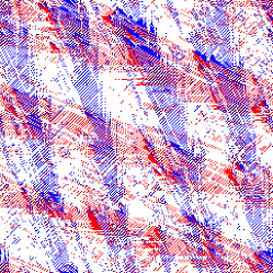
(b)

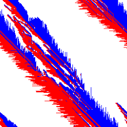
(c)

Figure 1: BML model on a $256\times 256$ lattice after $4096$ steps. (a) Free-flowing phase, $\rho=0.25$; (b) Intermediate phase, $\rho=0.32$; (c) Globally jammed phase, $\rho=0.38$. Red dots represent LR vehicles, while blue dots represent TB vehicles.

Despite its simplicity, the BML model undergoes a phase transition when the density $\rho$ of vehicles exceeds a critical value that depends on the grid size $N$ [1, 6]. When $\rho$ is below the critical threshold, the system stabilizes in a free-flowing state where vehicles arrange themselves in a non-interfering pattern to achieve maximum average speed. If the density is just above the critical threshold, a global jam eventually develops and no further movement is possible.

Figure 1 shows three configurations of the BML model after $4096$ steps (each step includes a horizontal and vertical phase) on a grid of size $256\times 256$ for different values of the vehicle density $\rho$. There are approximately $\rho N/2$ vehicles of each type that are initially placed randomly on the grid. Figure 1(a) shows the free-flowing state that arises when $\rho=0.25$. Increasing the vehicle density $\rho=0.32$ Figure 1(b) shows the intermediate phase that can be observed if the value of $\rho$ is increased, but is still below the critical threshold. When the density $\rho$ reaches the critical threshold, all vehicles are eventually stuck in a giant traffic jam as shown in Figure 1(c), and the average speed drops to zero. In fact, the behavior of the BML model is more complex: the free-flowing and jammed states might coexist, i.e., have non-zero probability to occur, when $\rho$ lies within some interval around the critical point [6].

The following rule can be used during a horizontal phase to compute the new state center’ of a cell, given its current state center and the current state of its left and right neighbors:

center’ $$=\begin{cases}\texttt{LR}&\text{if}\ \texttt{left}=\texttt{LR}\wedge\texttt{center}=\texttt{EMPTY}\\ \texttt{EMPTY}&\text{if}\ \texttt{center}=\texttt{LR}\wedge\texttt{right}=\texttt{EMPTY}\\ \texttt{center}&\text{otherwise}\end{cases}$$

Similarly, the following rule can be used to compute the new state of a cell during a vertical phase, given its current state and the state of its neighbors locate at the top and bottom:

center’ $$=\begin{cases}\texttt{TB}&\text{if}\ \texttt{top}=\texttt{TB}\wedge\texttt{center}=\texttt{EMPTY}\\ \texttt{EMPTY}&\text{if}\ \texttt{center}=\texttt{TB}\wedge\texttt{bottom}=\texttt{EMPTY}\\ \texttt{center}&\text{otherwise}\end{cases}$$

Two variations are described in the original paper [1], called Model II and Model III. Model II allows all vehicles to advance one step in the same phase; if a LR and TB vehicle try to occupy the same empty cell, one of them is randomly selected to move while the other stands still. Model III allows the same cell to contain both a LR and a TB vehicle. Both these models exhibit the same behavior of Model I.

The original BML model has been extended in several directions. Cámpora et al. [2] studied the behavior of the automaton on a square lattice embedded in a Klein bottle. Ding et al. [5] analyzed a different update rule where a randomly chosen vehicle is allowed to move at each step. Freund and Pöschel [7] proposed a more general automaton where vehicles can move in all directions and intersections are modeled more realistically. Other extensions of the BML model include [3]: asymmetric distribution of vehicles where the number of TB and LR vehicles is not the same; different speeds for TB and LR vehicles; two-level crossing to simulate the presence of overpasses and underpasses; permanent or transient road blocks, e.g., caused by traffic accidents.

3 Serial implementation

The BML model is a synchronous CA, since it requires that all cells are updated at the same time. To achieve this it is necessary to use two grids, say cur and next, holding the current and next CA configuration, respectively. Cell states are read from cur  and new states are written to next. When all new states have been computed, cur and next are exchanged.

Since the C language lays out 2D arrays row-wise in memory, it is easier to treat cur and next as 1D arrays, and use a function (or macro) IDX(i,j) to compute the mapping of the coordinates $(i,j)$ to a linear index. Therefore, we write cur[IDX(i,j)] to denote the cell at coordinates $(i,j)$ of cur. In case of a $N\times N$ grid, the function IDX(i,j) will return $(i\times N+j)$.

Since the BML model is a three-state CA, two bits would be sufficient to encode each cell. However, to simplify memory accesses we use one byte per cell. The following code defines all necessary data types, and shows how the horizontal phase can be realized (the vertical phase is very similar, and is therefore omitted).

⬇

typedef unsigned char cell_t;

enum {EMPTY = 0, LR, TB};

cell_t *cur, *next;

void horizontal_step(cell_t *cur, cell_t *next, int N) {

int i, j;

for (i=0; i<N; i++) {

for (j=0; j<N; j++) {

const cell_t left = cur[IDX(i,(j-1+N)%N)];

const cell_T center = cur[IDX(i,j)];

const cell_t right = cur[IDX(i,(j+1)%N)];

cell_t *out = &next[IDX(i,j)];

*out = (left == LR && center == EMPTY ? LR :

(center == LR && right == EMPTY ? EMPTY :

center));

}

}

}

void vertical_step(cell_t *cur, cell_t *next, int N) { ... }

A direct implementation of the BML morel uses grids of $N\times N$ elements. However, care must be taken when accessing the neighbors of cell $(i,j)$ to avoid out-of-bound accesses. A common optimization is to surround the domain with additional rows and columns, called ghost cells [9]. The domain becomes a grid of size $(N+2)\times(N+2)$, where the true domain consists of the cells $(i,j)$ for all $1\leq i\leq N+1$, $1\leq j\leq N+1$, while those on the border contain a copy of the cells at the opposite side (see Figure 2).

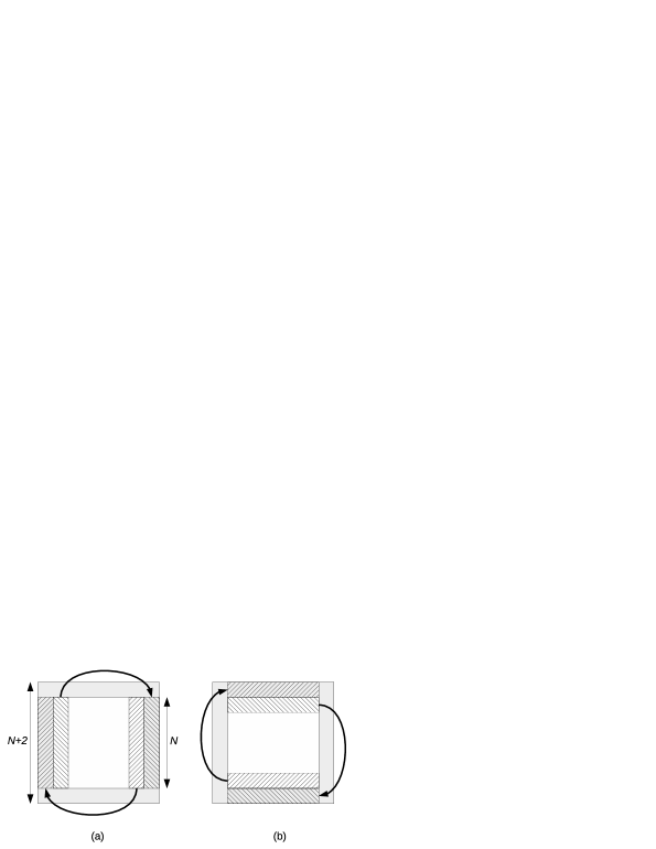
Figure 2: An $N\times N$ domain (white) augmented with ghost cells (gray). The corners of the extended domain are ignored, since they are not used by the BML update rules.

The top and bottom ghost rows must be filled before each vertical update phase (Fig. 2 (a)), while the ghost columns on the left and right must be filled before each horizontal phase (Fig. 2 (b)). Ghost cells simplify the indexing of neighbors and provide a significant speedup as will be shown in Section 7.

4 OpenMP implementation

OpenMP [4] is an open standard that supports parallel programming on shared-memory architectures; bindings for the C, C++ and FORTRAN languages are available. OpenMP allows the programmer to annotate portions of the code as parallel regions; the compiler generates the appropriate code to dispatch those regions to the processor cores.

In the C and C++ languages, OpenMP annotations are specified using #pragma preprocessor directives. One such directives is #pragma omp parallel for, that can be used to automatically distribute the iterations of a “for” loop to multiple cores, provided that the iterations are independent (this requirement must be verified by the programmer). The update loop(s) of the BML model can then be parallelized very easily as follows (we are assuming the presence of ghost cells, so that the indexed $i$ and $j$ assume the values $1,\ldots,N$).

⬇

...

#pragma omp parallel for

for (i=1; i<N-1; i++) {

for (j=1; j<N-1; j++) {

/* update cell (i,j) */

}

}

...

5 SIMD implementation

Modern processors provide SIMD instructions that can apply the same mathematical or logical operation to multiple data items stored in a register. A SIMD register is a small vector of fixed length (usually, 128 or 256 bits). Depending on the processor capabilities, a 128-bit wide SIMD register might contain, e.g., two 64-bit doubles, four 32-bit floats, four 32-bit integers, and so on.

Some applications can greatly benefit from SIMD instructions. However, there are some limitations: (i) SIMD instructions are processor-specific, and hence not portable. (ii) Automatic generation of SIMD instructions from scalar code is beyond the capabilities of most compilers and requires manual intervention from the programmer. (iii) SIMD instructions might impose constraints on how data is laid out in memory, e.g., by forcing specific alignments for memory loads and stores.

The SSE2 instruction set of Intel processors provides instructions that can operate on 16 chars packed into a 128-bit SIMD register. This allows us to compute the new states of 16 adjacent cells at the time. The SIMD version of the BML model has been realized using vector data types provided by the GNU C Compiler (GCC). Vector data types are a proprietary extension of GCC that allow users to use SIMD vectors as if they were scalars: the compiler emits the appropriate instructions to apply the desired arithmetic or logical operator to all the elements of the vector.

The conditional branches required to compute the next state of each cell are difficult to vectorize. The reason is that a branch may cause a different execution path to be taken for different elements of a SIMD register, which contrasts with the SIMD paradigm that requires that the same sequence of operations is applied to all data items. To overcome this problem we need to compute the new states using a technique called selection and masking, that makes use of bit-wise operations only. The idea is to replace a statement like a = (C ? x : y), where C is $0$ or $-1$ (0xffffffff in two’s complement, hexadecimal notation), with the functionally equivalent statement a = (C & x) | (~C & y), where the conditional branch no longer appears.

The code below defines a vector datatype v16i of 16 chars and uses it to compute the new state out of 16 adjacent cells at the time.

⬇

typedef char v16i __attribute__((vector_size(16)));

void horizontal_step(cell_t *cur, cell_t *next, int N) {

int i, j;

for (i=1; i<N+1; i++) {

for (j=1; j<(N+1)-15; j += 16) {

const v16i left = __builtin_ia32_loaddqu((char*)&cur[IDX(i,j-1)]);

const v16i center = __builtin_ia32_loaddqu((char*)&cur[IDX(i,j)]);

const v16i right = __builtin_ia32_loaddqu((char*)&cur[IDX(i,j+1)]);

const v16i mask_lr = ((left == LR) & (center == EMPTY));

const v16i mask_empty = ((center == LR) & (right == EMPTY));

const v16i mask_center = ~(mask_lr | mask_empty);

const v16i out = ((mask_lr & LR) | (mask_empty & EMPTY) | \

(mask_center & center));

__builtin_ia32_storedqu((char*)&next[IDX(i,j)], out);

}

}

}

left, center and right can be thought as C arrays of length 16 holding the values of the left, center, and right neighbors of 16 adjacent cells. Their contents are fetched from memory using the __builtin_ia32_loaddqu (Load Double Quadword Unaligned) intrinsic (again we are assuming that the domain is extended with ghost cells).

The mask_lr, mask_empty and mask_center vector variables contain the value $-1$ in the positions where LR, EMPTY and center should be stored, respectively. Note that the compiler automatically converts scalars to vectors, to handle mixed comparisons like (left == LR). Conveniently, SSE2 comparison instructions generate the value $-1$ (instead of $1$) for true. The new states out of the 16 cells can then be computed using bit-wise operators that the compiler translates into a sequence of SIMD instructions. The result is stored back in memory using the __builtin_ia32_storedqu (Store Double Quadword Unaligned) intrinsic.

6 CUDA implementation

A modern GPU contains a large number of programmable processing cores that can be used for general-purpose computing. The first widely used framework for GPU programming has been the CUDA toolkit by NVidia corporation. A CUDA program consists of a part that runs on the CPU and one that runs on the GPU. The source code is annotated using proprietary extensions to the C, C++ or FORTRAN programming languages that are understood by the nvcc compiler. Recently, CUDA has evolved into an open standard called OpenCL that is supported by other vendors; however, in the following we consider CUDA since is currently more robust and efficient than OpenCL.

The basic unit of work that can be executed on a CUDA-capable GPU is the CUDA thread. Threads can be arranged in one-, two-, or three-dimensional blocks, that can be further assembled into a one-, two-, or three-dimensional grid. Each thread has unique identifiers that can be used to map a thread to one input element. The CUDA paradigm favors decomposition of a problem into very small tasks that are assigned to threads (fine-grained parallelism). The CUDA runtime schedules threads to cores for execution; the hardware supports multitasking with almost no overhead, so that the number of threads can (and usually does) exceed the number of cores.

Implementation of the BML model with CUDA is quite simple, and consists of transforming the horizontal_step and vertical_step functions to CUDA kernels, i.e., blocks of code that can be executed by a thread. CUDA kernels are designated with the __global__ specifier. Using two-dimensional blocks of threads it is possible to assign one thread to each element $(i,j)$; this requires launching $N\times N$ threads. The horizontal_step function becomes a CUDA kernel as follows:

⬇

__global__

void horizontal_step(cell_t *cur, cell_t *next, int N) {

const int i = 1 + threadIdx.y + blockIdx.y * blockDim.y;

const int j = 1 + threadIdx.x + blockIdx.x * blockDim.x;

if ( i < N+1 && j < N+1) {

/* update cell (i,j) */

}

}

CUDA cores have no direct access to system RAM; instead, they can only use the GPU memory, called device RAM. Therefore, input data must be transferred from system RAM to device RAM before the CUDA threads are activated. Once computation on the GPU is completed, output data is transferred back to system RAM. The parameters cur and next above point to device RAM.

7 Performance evaluation

Table 1: Hardware used for the experimental evaluation

	Machine A	Machine B
CPU	Intel Xeon E3-1220	Intel Xeon E5-2603
Cores	4	12
HyperThreading	No	No
Max CPU freq.	3.50 GHz	1.70 GHz
L2 Cache	256 KB	256 KB
L3 Cache	8192 KB	15360 KB
RAM	16 GB	64 GB
GPU	Quadro K620	GeForce GTX 1070
GPU max clock rate	1.12 GHz	1.80 GHz
Device RAM	1993 MB	8114 MB
CUDA cores	384	1920

In this section we compare the implementations of the BML automaton described so far: the scalar version without ghost cells from Section 3 (serial); the serial version with ghost cells (Serial+halo); the OpenMP version from Section 4 (OpenMP); the SIMD version from Section 5 (SIMD); a combined OpenMP+SIMD version, where cells are updated using SIMD instructions and the outer loops are parallelized with OpenMP directives (OpenMP+SIMD); finally, the CUDA version from Section 6 (CUDA). In the cases where OpenMP is used, we make use of all processor cores available in the machine.

All implementations have been realized under Ubuntu Linux version 16.04.4 using GCC 5.4.0 with level 3 optimization enabled using the compiler flags -O3 -march=native; the CUDA version has been compiled with the proprietary nvcc compiler from the CUDA Toolkit version 9.1. We run the programs on two multi-core machines equipped with CUDA capable GPUs, whose specifications are shown in Table 1. Machine A has a fast, four-core processor but includes a low-end GPU. Machine B has a more powerful GPU and a processor with twelve cores; however, each core runs at a lower clock rate.

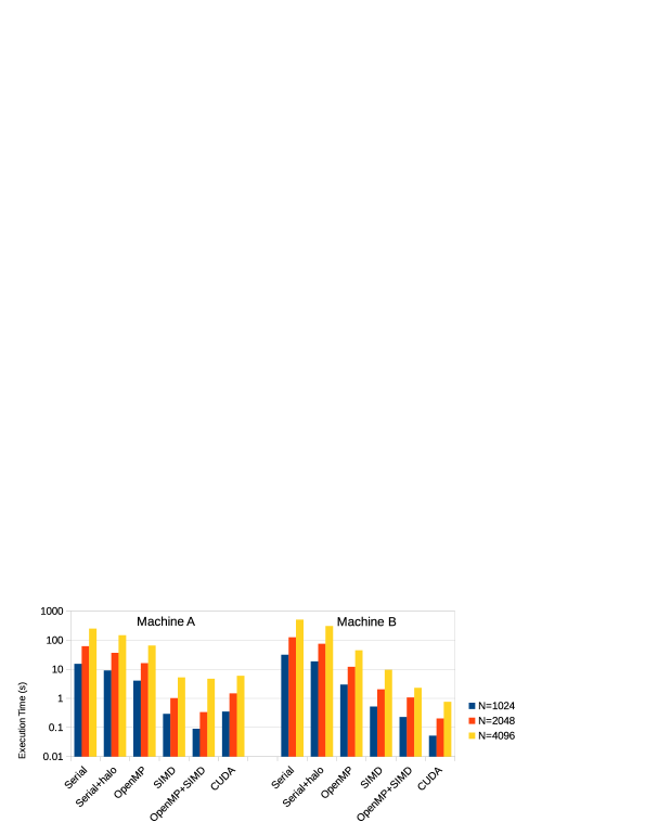
	Machine A			Machine B
$N$	$1024$	$2048$	$4096$	$1024$	$2048$	$4096$
Serial	15.446	61.957	249.026	31.554	126.298	508.046
Serial+halo	9.091	36.545	148.266	18.725	75.046	304.818
OpenMP	4.080	16.256	65.366	2.988	12.184	44.763
SIMD	0.294	1.021	5.252	0.524	2.044	9.652
OpenMP+SIMD	0.090	0.339	4.730	0.228	1.079	2.292
CUDA	0.351	1.482	5.970	0.052	0.202	0.768

Figure 3: Mean execution time of BML model implementations ($\rho=0.3$, $1024$ steps)

The BML automaton has been simulated with a vehicle density $\rho=0.3$ on a domain of size $N\times N$, $N=1024,2048,4096$ for $1024$ steps. Figure 3 shows the execution time of each program; each measurement is the average of five execution. Note the logarithmic scale of the vertical axis, which is necessary since the execution times vary more than two orders of magnitude.

The use of ghost cells provides a significant reduction of the execution time (about 40%) compared to the use of the modulo operator; note how a simple modification can make such a difference. The OpenMP version using all available processor cores provides an additional speedup of about $2\times$ for machine A and about $6\times$ for machine B (recall that machine B has more cores). These speedups come very cheaply: the OpenMP version differs from the serial implementation by a couple of #pragma omp parallel for directives that have been added to the functions computing the horizontal and vertical steps.

The SIMD implementation provides perhaps the most surprising results. On machine A, a single core delivers more computing power than the mid-range GPU installed; by combining OpenMP and SIMD instructions it is possible to further reduce the execution time. On machine A the OpenMP+SIMD version is more than four times faster than the GPU for $N=1024,2048$; however, the gap closes for the larger domain size $N=4096$. Machine B has a slower CPU and a better GPU, so the GPU version is four to five times faster than the OpenMP+SIMD version.

8 Conclusions

In this paper we have analyzed the impact of several implementations of the BML traffic model on modern CPUs and GPUs. Starting with a serial version, we have applied the ghost cells pattern to reduced the overhead caused by the access to the neighbors of each cell. A parallel version has then been derived by applying OpenMP preprocessor directives to the serial implementation, to take advantage of multicore processors. More effort is required to restructure the code to take advantage of SIMD instructions; the payoff is however surprising: the SIMD version running on a single CPU core proved to be faster than a GPU implementation running on a mid-range graphic card.

The results suggest that traffic models can greatly benefit from accurately tuned CPU implementations, especially considering that a fast CPU can execute this type of workload faster than an average GPU. However, the most useful optimization, namely, the use of SIMD instructions, requires technical knowledge that the average user is unlikely to possess. It is therefore advised that traffic simulators and other CA modeling tools make these features available to the scientific community.

We are extending the work described in this paper by considering more complex and realistic traffic models based on CA. We expect that the findings reported above will still apply, at least to a certain extent, to any discrete CA.

References

- [1] Biham, O., Middleton, A.A., Levine, D.: Self-organization and a dynamical transition in traffic-flow models. Phys. Rev. A 46(10), R6124–R6127 (Nov 1992). https://doi.org/10.1103/PhysRevA.46.R6124
- [2] Cámpora, D., de la Torre, J., Vázquez, J.C.G., Caparrini, F.S.: BML model on non-orientable surfaces. Physica A: Statistical Mechanics and its Applications 389(16), 3290–3298 (2010). https://doi.org/10.1016/j.physa.2010.03.037
- [3] Chowdhury, D., Santen, L., Schadschneider, A.: Statistical physics of vehicular traffic and some related systems. Physics Reports 329(4), 199–329 (May 2000). https://doi.org/10.1016/S0370-1573(99)00117-9
- [4] Dagum, L., Menon, R.: OpenMP: An industry-standard API for shared-memory programming. IEEE Comput. Sci. Eng. 5, 46–55 (January 1998). https://doi.org/10.1109/99.660313
- [5] Ding, Z.J., Jiang, R., Wang, B.H.: Traffic flow in the Biham-Middleton-Levine model with random update rule. Phys. Rev. E 83, 047101 (Apr 2011). https://doi.org/10.1103/PhysRevE.83.047101
- [6] D’Souza, R.M.: Coexisting phases and lattice dependence of a cellular automaton model for traffic flow. Phys. Rev. E 71, 066112 (Jun 2005). https://doi.org/10.1103/PhysRevE.71.066112
- [7] Freund, J., Pöschel, T.: A statistical approach to vehicular traffic. Physica A: Statistical Mechanics and its Applications 219(1), 95–113 (Sep 1995). https://doi.org/10.1016/0378-4371(95)00170-C
- [8] Gutowitz, H. (ed.): Cellular Automata: Theory and Experiment. MIT Press (1991)
- [9] Kjolstad, F.B., Snir, M.: Ghost cell pattern. In: Proceedings of the 2010 Workshop on Parallel Programming Patterns. pp. 4:1–4:9. ParaPLoP ’10, ACM, New York, NY, USA (2010). https://doi.org/10.1145/1953611.1953615
- [10] Lee, V.W., Kim, C., Chhugani, J., Deisher, M., Kim, D., Nguyen, A.D., Satish, N., Smelyanskiy, M., Chennupaty, S., Hammarlund, P., Singhal, R., Dubey, P.: Debunking the 100x GPU vs. CPU myth: An evaluation of throughput computing on CPU and GPU. In: Proceedings of the 37th Annual International Symposium on Computer Architecture. pp. 451–460. ISCA ’10, ACM, New York, NY, USA (2010). https://doi.org/10.1145/1815961.1816021
- [11] Maerivoet, S., Moor, B.D.: Cellular automata models of road traffic. Physics Reports 419(1), 1–64 (2005). https://doi.org/10.1016/j.physrep.2005.08.005