Quantum Phase transitions in the two dimensional ionic-Hubbard model

Abstract

We employ the dynamical mean field approximation to study the effects of ionic potential ($\Delta$) on the square lattice Hubbard model. At half-filling when the staggered potential ($\Delta$) dominates the on-site Hubbard interaction ($U$), the system is in the band insulator phase. We find that competition between $U$ and $\Delta$ can suppress the gap to zero and leading to an intermediate metallic region. At the large-$U$ limit, we identify a Mott insulator phase where the gap opens again and increases upon increasing the Hubbard interaction U. For $U\leq 9t$ and $\Delta\approx 0$ the phase of the system is metallic, but for larger $U$ the system is in the Mott insulator phase.

1 Introduction

There are many quantum phase transitions which are driven by interactions. The metal-insulator transition [1, 2] and semi metal-insulator transition [3] serve as two examples. A famous model exhibiting competing interaction terms is the ionic Hubbard model (IHM), which includes a nearest-neighbour hopping, an on-site repulsive interaction, and a staggered potential which separates neighbouring sites by an energy shift [4]. When the staggered potential dominates, a band insulator results. In a bipartite lattice, the substrate can include a sub-lattice symmetry breaking (by ionic potential $\Delta$) so the ground state of this system will be a band insulator. The interaction can suppress the gap in the Band Insulators (BI) phase, by increasing repulsion interaction the energy gap would be created again [5]. On the strongly correlated limit, when the Hubbard term dominates over the ionic term in IHM, i.e. $U\gg\Delta$, the system goes to Mott insulator phase. In this limit, charge fluctuation is frozen and no double occupancy is expected. In higher dimensions, many theoretical and numerical analysis are published which investigate transition between Mott insulator and band insulator phases in the Ionic Hubbard Model (IHM). Many groups have applied the dynamical mean field theory (DMFT) [5, 6], detrimental quantum Monte carlo (DQMC) [8] and cluster dynamical mean field theory (CDMFT) [9] on IHM to studying the phase diagrams of mono layer or bilayer structures [10]. We know that the real ground state of the 2D square lattice could be in anti-ferromagnetic (AF) phase [7]; These numerical results of the DMFT equations for the IHM provides the existence of a critical interaction strength for the transition from a correlated BI to a MI. They found that the ground state of the system is always insulating. Their results shown there is a direct transition between the BI and the AF-MI [7]. We present results on the two dimensional square lattice ionic Hubbard model obtained by iterated perturbation theory (IPT) based DMFT [5]. The DMFT approach is one of the most powerful methods to study strongly correlated systems. In this method an impurity problem should be solved: the interaction between a single site of a lattice hybridized to a bath; The bath of non-interacting electrons must be determined self-consistently. The DMFT is a powerful method [1] which is capable of handling both the ionic and the Hubbard interaction term in IHM. This approximation becomes exact in limit of infinite coordination numbers. For lower coordination number, the local self-energy (k-independent) becomes only an approximate description. Therefore the most significant drawback of this approximation is expected to be underestimation of the spatial quantum fluctuations  [3, 12, 13, 14], hence the values of the critical phase transition parameters maybe overestimated [15]. But the overall picture emerging from a simple DMFT method is expected to hold even when more complicated methods are employed, such as CDMFT [16]. The DMFT were used in analysis the phase diagram of the Bethe lattice. The existence of metallic phase between the BI and MI phase has been proved [5]. The bilayer Hubbard model indicates a phase diagram similar to the IHM. This is because a large inter-layer coupling results in a BI similar to the large staggered potential limit of the IHM [17]. This problem could be generalized to the heterostructures such as $SrTiO3$ and $LaTiO3$, studies on these materials demonstrated a metallic phase appearing at the interface between a MI and BI phase [9]. In this manuscript, we first introduced the IHM model and DMFT technique with IPT impurity solver in section II, in Section III we present the results and discussions on the DMFT phase diagram in the $\Delta$-$U$ plane. We end this manuscript by giving a conclusion in section IV.

2 Model and Method

The 2D ionic-Hubbard model on a bipartite (two sub-lattices A and B) square lattice is given by

$$H=-t\sum_{i\epsilon A,j\epsilon B,\sigma}(c_{i\sigma}^{{\dagger}}c_{j\sigma}+h.c.)-\Delta\sum_{i\epsilon A}{n_{i}}+\Delta\sum_{i\epsilon B}{n_{i}}$$

$$+U\sum_{i}n_{i\uparrow}n_{i\downarrow}-\mu\sum_{i\sigma}n_{i}$$ (1)

where $t$ denotes the nearest neighbour hopping and $c_{i\sigma}^{{\dagger}}(c_{i\sigma})$ are the creation (annihilation) operator of electrons at site $i$ with spin $\sigma$. $\Delta$ is the ionic staggered potential which alternates sign between sites in sub-lattice $A$ or $B$. The number operator is $n_{i,\sigma}$ which determines the number of electrons at site $i$ with projection of spin $\sigma$. The chemical potential is $\mu=U/2$ at half filling and $U$ designates the on-site electron-electron repulsion Hubbard potential. We take $t$ as the energy unit through out this paper, we will consider the average filling factor $\frac{\langle n_{A}\rangle+\langle n_{B}\rangle}{2}=1$.

In this model for $t>0$ and non-interacting limit $U=0$, a band insulator phase represents with energy gap, $E_{gap}=2\Delta$. The sites $A(B)$ have potential $-\Delta(\Delta)$ , respectively. The electrons prefer to doubly occupy lower bands Fig.1. The average filling factors at half-filling is $\langle n_{A}\rangle=2$, $\langle n_{B}\rangle=0$ at $U=0$ and $t=0$.

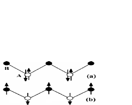
Figure 1: (Color online) The comparison between electrons occupancy on sites $A$ and $B$ in BI and MI phase. The $A$ sites have lower potential than $B$ sites. $(a)$ In band insulator the electrons choose doubly occupy lower bands. $(b)$ In Mott insulator phase the electrons prefer to occupy only one sites, $A$ and $B$.

In other limit, for $U\gg\Delta$, the system goes to MI phase with $\langle n_{A}\rangle=\langle n_{B}\rangle=1$ [18]. The flow equation methods predicted in the intermediate region at some energy scales the ionic and Hubbard potentials can cancel each other’s effect  [18]. From this point of view the tight-binding term dominates the nature of the ground state. Therefore we expect the intermediate phase to be a metal [5, 18]. Here we study the IHM using the DMFT approach [5]. To formulate the DMFT machinery, first we consider IH Hamiltonian on the square lattice in $\it{paramagnetic~{}phase}$. The interaction Green’s function in the bipartite lattice are,

$$G^{-1}(\vec{k},\omega^{+})=\left(\begin{array}[]{ll}\zeta_{A}(\vec{k},\omega^{+})&-\epsilon(\vec{k})\\ -\epsilon(\vec{k})&\zeta_{B}(\vec{k},\omega^{+})\\ \end{array}\right)$$ (2)

where $\vec{k}$ is the momentum vector in first Brillouin zone (FBZ), $\epsilon(\vec{k})=\epsilon(k_{x},k_{y})=-2t(cos(k_{x})+cos(k_{y}))$ is the energy dispersion for square lattice, and $\zeta_{A(B)}=\omega^{+}\mp\Delta+\mu+\sum_{A(B)}(\omega^{+})$ with $\omega^{+}=\omega+i0^{+}$. The self-energy, $\sum_{\alpha}(\omega^{+})$ in DMFT is local and independent of $\vec{k}$. The matrix elements of the self energy are diagonal and the off-diagonal elements are zero. The local Green’s function of two sub-lattices could be written as, $G_{\alpha}(\omega^{+})=\sum_{\vec{k}}G_{\alpha\alpha}(\vec{k},\omega^{+})$,

$$G_{\alpha}(\omega^{+})=\zeta_{\bar{\alpha}}(\omega^{+})\int_{-\infty}^{\infty}d\epsilon\frac{\rho_{0}(\epsilon)}{\zeta_{A}(i\omega_{n})\zeta_{B}(i\omega_{n})-\epsilon^{2}}$$ (3)

where for $\alpha=A(B)$, $\bar{\alpha}=B(A)$. The bare density of state obtained for the square lattice,

$$\rho_{0}(\epsilon) = \frac{1}{2t\pi^{2}}\int_{0}^{\pi}dk_{x}\int_{0}^{\pi}dk_{y}\delta(\tilde{\epsilon}+cos(k_{x})+cos(k_{y}))$$ (4)

$$= \frac{1}{2t\pi^{2}}\int_{-1}^{1}d{x}\int_{-1}^{1}dy\frac{\delta(\tilde{\epsilon}+x+y)}{\sqrt{(1-x^{2})(1-y^{2})}}$$

$$= \frac{1}{2t\pi^{2}}\int d{x}\frac{1}{\sqrt{(1-x^{2})(1-(\tilde{\epsilon}+x)^{2})}}$$

where $\tilde{\epsilon}=\epsilon/2t$. The Eq. 4 can be evaluated numerically for these two intervals, $-1\leq x\leq 1$ and $-1\leq(\tilde{\epsilon}+x)\leq 1$. We first guess the initial filling factor and self-energy [5]. Then we determine the host Green’s function from the Dyson’s equation $\mathcal{G}_{0\alpha}^{-1}(\omega^{+})=G_{\alpha}{-1}(\omega^{+})+\sum_{\alpha}(\omega^{+})$. Afterwards, we solve impurity problem and obtain $\sum_{\alpha}(\omega^{+})=\sum_{\alpha}(\mathcal{G}_{0\alpha}(\omega^{+}))$. We use IPT method as impurity solver [5]. The iteration in these steps continues until convergence is reached. We calculate the density of state by $\rho_{\alpha}(\omega)=-\sum_{\vec{k}}\Im[G_{\alpha}(\vec{k},\omega^{+})]/\pi$. From the particle-hole symmetry at half-filling we obtain $\rho_{A}(\omega)=\rho_{B}(-\omega)$ for the $DOS$ of two sub-lattices. The total $DOS$ for square lattice obtains via $\rho(\omega)=\rho_{A}(\omega)+\rho_{B}(\omega)$.

3 Results and Discussions

3.1 DOS

In Fig. 2 has been showed the DOS for some values of $U$ at a constant $\Delta=0.3t$. This figure can covers the whole range of energies. For small values of $U$ ($U\leq U_{c1}$) the spectrum has simple gap. By increasing $U$ ($U_{c1}\leq U\leq U_{c2}$), the overall feature of the low energy spectrum changes and the DOS around $\omega=0$ has singularity and the gap was closed. When $U$ increases ($U\geq U_{c2}$) we see the upper and lower Hubbard band appear, symmetrically. The formation of the Hubbard bands are shown in Fig. 2.

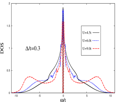
Figure 2: (Color online) The density of states for square lattice in IHM are plotted for $U=4.5t,~{}6.0t,~{}9.0t$, $\Delta=0.3t$. In this figure, the Hubbard bands appeared symmetrically in both sides of $\omega=0$.

The DOS of square lattice in Hubbard model ($\Delta=0$) has Van-Hov singularity around the Fermi level. When the ionic potential ($\Delta$) was added, at $U=0$ the energy gap is $E_{gap}\simeq 2\Delta$, and two singularities was appear in both sides of the gap. By increasing $U$ in $U\leq U_{c1}$ interval the Van-Hov singularities moves towards lower energies. In $U\geq U_{c2}$ interval singularities move towards higher energies.

3.2 $E_{gap}$

The energy gap could be calculated in two methods, first through measurement the gap of DOS, second from the formula of $E_{gap}$,

$$E_{gap}=Z|\Delta-U\delta n/2+S|$$ (5)

Where $Z$ is independent of $\alpha$, $\delta n=\frac{\langle n_{A}\rangle-\langle n_{B}\rangle}{2}$ and $S=P\int_{-\infty}^{\infty}d\omega\sum^{\prime\prime}_{A}(\omega)/\pi\omega$. We could find the gap strongly depends on repulsion interaction 3. In Fig. 3, the dots diagram obtained from measurement the energy gap from the DOS and the open square with error bars obtained from Eq. 5 for $\Delta=0.5t$. The inner figure is plotted for $\Delta\simeq 0$. We found that at $\Delta=0$ the gap is opened in $U>U^{0}_{c}$ interval ($U^{0}_{c}\geq 9t$). This is not in accordance with the results of Ref. [8] in $\Delta\simeq 0$ which used determinant quantum Monte Carlo (DQMC) method. As can be seen the actual (interacting) gap strongly depends on the interaction parameter U in BI and MI phases. The DOS and error bars diagrams have excellent agreement with each other in both figures.

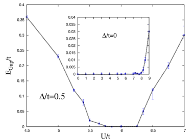
Figure 3: (Color online) The energy gap for $\Delta/t=0.5$ with two methods plotted $vs$ $U$ in unit of $t$. The gap (dots) is plotted using the DOS. The results with error bars (open square) obtained from Eq. 5. The error bars related to numerical errors in calculation of $\sum^{\prime\prime}(\omega)$ at small $\omega$ [5]. The inner figure shows $E_{gap}$ in $\Delta/t=0$.

The error bars estimated from calculation of $\sum^{\prime\prime}(\omega\rightarrow 0)$. We increased the accuracy of the calculations and we used accurate methods in numerical integration. These error bars obtained by considering these two results from two integration methods.

3.3 Self-Energy

For more Discussions in the scale of energy gap we consider the self energy of this system, $\sum_{\alpha}(\omega^{+})=\sum^{\prime}_{\alpha}(\omega)+i\sum^{\prime\prime}_{\alpha}(\omega)$, where shape of imaginary part of self energy can show insulating or metallic phase of systems [5, 12]. The $\sum^{\prime\prime}_{A}(\omega)$ vanishes around $\omega=0$ in BI and MI phases, according to the Fermi liquid theory in metallic phase $\sum^{\prime\prime}_{A}(\omega)=\omega^{2}$ [5]. We showed these results in Fig. 4.

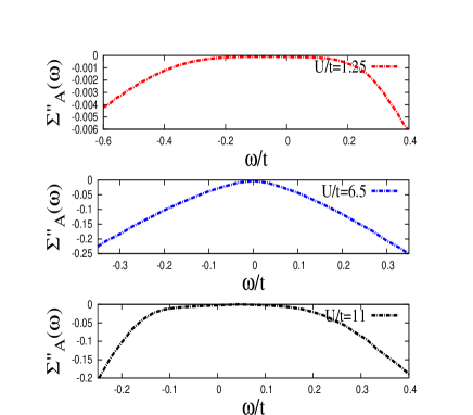
Figure 4: (Color online) The Imaginary part of self energy for $\Delta/t=0.1$ plotted $vs$ $\omega$. The top and low panel are related to Band insulator and Mott insulator. The middle panel is related to Metallic phase.

3.4 Phase diagram

By repeating the calculation for wide range of Hubbard potential and ionic potential, we can map out the phase diagram of the square lattice for ionic-Hubbard model. When $\Delta=0$, IHM is reduced to the Hubbard model. As it is known [11] for the Hubbard model on the square lattice for finite values of $U$ according to the DMFT, phase transition takes place from metallic to MI phase. We could find interesting results different from phase diagram of honeycomb lattice. The phase of the honeycomb lattice in $\Delta=0$ and finite $U$, is semi-metal [12]. In $\Delta>>0$ region the metallic region shrinks to a single metallic point for honeycomb lattice. But in the 2D square lattice for $\Delta\approx 0$, the only critical repulsion potential is $U_{c}\approx 9.1t$. In the range of $U\leq 9.1t$, the metallic phase is dominate. By increasing the amount of $U$ in $\Delta\approx 0$ the MI phase is overcome 5.

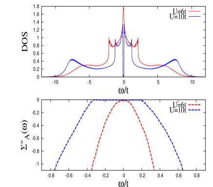
Figure 5: (Color online) The DOS and imaginary part of self energy of square lattice for $\Delta/t=0$ and $U/t=6~{},10$ are plotted $vs$ $\omega$. The top and low panel are related to DOS and $\sum^{\prime\prime}_{A}$ respectively.

It is well known that, phase transition from metallic to insulating phase for Hubbard model ($\Delta=0$) is the first order. We could find coexistence region of metallic and insulating phase at finite $\Delta$, last Ref. in  [11]. In the square lattice a little increasing in $U\simeq 9.1t$ for $\Delta\approx 0$ can open the gap, this could be explained as the easiness the phase transition of Schrödinger electrons compared to Dirac electrons [3]. If we employ the DMFT to the IHM at zero temperature allowing for spontaneous AF long-range order, We find that the ground state is always insulating phase with a gap in DOS. We could find a direct transition between the BI and the AF-MI [7]. In Ref. [8] at $\Delta=0$ we could not see the phase transition and the system is in Mott insulator phase. But DMFT gives metallic phase for finite $U$ which is the mean-field artefact. The inclusion of inter-site magnetic fluctuations could be yield an anti-ferromagnetic insulating phase for all U (in DQMC method) on the two dimensional systems.

But our results are obtained in the paramagnetic phase as ground state. One can expect that the metallic phase will survive if AF is suppressed due to frustration, in the same way as in the DMFT treatment in the $\Delta=0$ limit [1]. In future work we could consider a model in which such frustration is explicitly included.

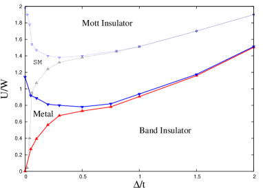
Figure 6: (Color online) The phase diagram of IHM on the square lattice by DMFT(IPT) method. The metallic phase is between two insulator phases. We plotted the phase diagram of honeycomb lattice in competition with square lattice.

Our results in prediction of phase transition in $\Delta\approx 0$ have nearly good agreement with results obtained from other DMFT methods on Hubbard model ($\Delta=0$) [11]. For IHM on the square lattice at finite temperature [19] and on Bethe lattice at $T=0$  [5] show that for $\Delta\approx 0$ and $\Delta\ll 1$ phase transition from metallic to MI phases take place. In this paper, three phases BI, MI and Metal are predicted at zero temperature $T=0$. The w is bandwidth. But if the temperature increased $e.g.$ $k_{B}T=0.01$, the phase diagram will be changed [19]. In Ref. [19] for $\Delta\approx 0$ and $0<U<U_{c1}\simeq 2$ the 2D square lattice is in Metallic phase. Similar studies have been done on bilayer square lattice IHM with interesting results [20]. For large $\Delta$ we can consider that the metallic region goes to the narrow metallic region, which has good agreement with [19].

Our results in small $\Delta$ have good agreement with Ref. [11] which used Hubbard model. The changes of regions in phase diagrams of the systems in $\Delta\geq 1$ could be compared with [19] that the metallic region becomes narrow. We plotted the phase diagram of honeycomb lattice in Fig. 6. The two systems have same treatment in quantum phase transition, but the middle phase is semi-metal(SM) in the honeycomb lattice.

4 Conclusion

We studied the ionic-Hubbard model on 2D square lattice by IPT impurity solver. We calculated density of state, energy gap and self-energy at $T=0$ conditions. Our results show a metallic phase is between to insulator phases. For $\Delta>0$ the system is in band insulator ($0<U<U_{c1}(\Delta)$). By increasing $U$ in $U_{c1}(\Delta)<U<U_{c2}(\Delta)$ region, the system shows metallic character. Finally, for $U>U_{c2}(\Delta)$ the correlations transform the metallic phase to Mott Insulator. The calculations showed by increasing $\Delta$ the metallic region becomes narrow.

5 Acknowledgements

We would like to thank M. Hafez Torbati for many useful discussions.

References

- [1] A. Georges, G. Kotliar, W. Krauth, and M. J. Rozenberg, Rev. Mod. Phys. 68, 13 (1996).
- [2] T. Pruschke, M. Jarrell, and J. K. Freericks, Adv. Phys. 44, 187 (1995).
- [3] M. Ebrahimkhas, Phys. Lett. A, 375 (2011) 3223.
- [4] J. Cho, JW. Lee, Journal of the Korean Physical Society, 70, 494 (2017).
- [5] A. Garg, H. R. Krishnamurthy, and M. Randeria, Phys. Rev. Lett. 97, 046403 (2006); A. Garg, H. R. Krishnamurthy, and M. Randeria, Phys. Rev. Lett. 112, 106406 (2014).
- [6] L. Craco, P. Lombardo, R. Hayn, G. I. Japaridze, and E. Muller-Hartmann, Phys. Rev. B 78, 075121 (2008).
- [7] Krzysztof Byczuk, Michael Sekania, Walter Holfstetter, and Arno P. K. Kampf, Phys. Rev. B 79, 121103 (2009).
- [8] K. Bouadim, N. Paris, F. Hebert, G. G. Batrouni, and R. T. Scalettar, Phys. Rev. B 76, 085112 (2007); N. Paris, K. Bouadim, G. G. Batrouni, and R. T. Scalettar, Phys. Rev. Lett. 98, 046403 (2007);
- [9] S. S. Kancharla and E. Dagotto, Phys. Rev. Lett. 98, 016402 (2007).
- [10] R. Ruger, L. F. Tocchio, R. Valenti and C. Gros, New J. Phys. 16, 033010 (2014).
- [11] T. Schafer, F. Geles, D. Rost, G. Rohringer, E. Arrigoni, K. Held, N. Blumer, M. Aichhorn, A. Toschi, Phys. Rev. B 91, 125109 (2015); T. Ayral, O. Parcollet, Phys. Rev. B 93, 235124 (2016); L. Fratino, P. S ̵́emon, M. Charlebois, G. Sordi, A.-M. S. Tremblay, Phys. Rev. B 95, 235109 (2017); Helena Braganca, Shiro Sakai, M. C. O. Aguiar, M. Civelli, Phys. Rev. Lett. 120 067002 (2018).
- [12] M. Ebrahimkhas, Z. Drezhegrighash, E. Soltani, Phys. Lett. A, 379, 1053 (2015); M. Ebrahimkhas, S. A. Jafari, Eur. Phys. Lett. 98 27009 (2012). M. Ebrahimkhas; S. A. Jafari, Eur. Phys. J. B 68, 537 (2009).
- [13] S. A. Jafari, Eur. Phys. J. B 68, 537 (2009).
- [14] Minh-Tien Tran and Kazuhiko Kuroki,Phys. Rev. B, 79, 125125 (2009).
- [15] Wei Wu, Yao-Hua Chen, Hong-Shuai Tao, Ning-Hua Tong, and Wu-Ming Liu, Phys. Rev. B 82, 245102 (2010).
- [16] A. Liebsch, Phys. Rev. B, 83, 035113 (2010).
- [17] S. Okamoto and A. J. Millis, Phys. Rev. B 70, 075101 (2004); S. S. Kancharla and S. Okamoto, Phys. Rev. B 75, 193103 (2007); K. Maiti, R. Shankar Singh and V. R. R. Medicherla, Phys. Rev. B 76, 165128 (2007).
- [18] M. Hafez, S. A. Jafari, M. A. Abolhssani, Phys. Lett. A 373, 4479 (2009).
- [19] B. Martinie, cond-mat/10020325 (2010).
- [20] M. Jiang and T. C. Schulthess, Phys. Rev. B 93, 165146 (2016); M. Jiang and T. C. Schulthess, cond-mat/160403271 (2016).