Viscous Overstability in Saturn’s Rings: Influence of Collective Self-gravity

Abstract

We investigate the influence of collective self-gravity forces on the nonlinear, large-scale evolution of the viscous overstability in Saturn’s rings. We numerically solve the axisymmetric nonlinear hydrodynamic equations in the isothermal and non-isothermal approximation, including radial self-gravity and employing transport coefficients derived by Salo et al., (2001). We assume optical depths $\tau=1.5-2$ to model Saturn’s dense rings. Furthermore, local N-body simulations, incorporating vertical and radial collective self-gravity are performed. Vertical self-gravity is mimicked through an increased frequency of vertical oscillations, while radial self-gravity is approximated by solving the Poisson equation for an axisymmetric thin disk with a Fourier method. Direct particle-particle forces are omitted, which prevents small-scale gravitational instabilities (self-gravity wakes) from forming, an approximation that allows us to study long radial scales and to compare directly the hydrodynamic model and the N-body simulations. Our isothermal and non-isothermal hydrodynamic model results with vanishing self-gravity compare very well with results of Latter and Ogilvie, (2010) and Rein and Latter, (2013), respectively. In contrast, for rings with radial self-gravity we find that the wavelengths of saturated overstable waves settle close to the frequency minimum of the nonlinear dispersion relation, i.e. close to a state of vanishing group velocities of the waves. Good agreement is found between non-isothermal hydrodynamics and N-body simulations for moderate and strong radial self-gravity, while the largest deviations occur for weak self-gravity. The resulting saturation wavelengths of viscous overstability for moderate and strong self-gravity ($\lambda\sim 100-300\text{m}$) agree reasonably well with the length scales of axisymmetric periodic micro-structure in Saturn’s inner A-ring and the B-ring, as found by Cassini.

December 19, 2017

1 Introduction

Observational evidence for the presence of axisymmetric periodic micro-structure on length scales of $100\,\text{m}-200\,\text{m}$ in Saturn’s A and B rings was revealed by several instruments onboard the Cassini mission to Saturn. The structure was seen in radio occultations performed by the Radio Science Subsystem (RSS) (Thomson et al., (2007)) and stellar occultations carried out with the Ultraviolet Imaging Spectrograph (UVIS) (Colwell et al., (2007);  Sremcevic et al., (2009)). The axisymmetric nature of oscillations was demonstrated by the Visual and Infrared Mapping Spectrometer (VIMS) occultations analysed by Hedman et al., (2014), indicating azimuthal coherence of the wave trains over length scales of thousands of kilometers. To date, this micro-structure is best explained by axisymmetric waves induced in the rings by viscous overstability.

Since the work of Schmit and Tscharnuter, (1995, 1999) an increasing amount of effort has been devoted to theoretical as well as simulational studies of the spontaneous viscous overstability in Saturn’s rings. Schmit and Tscharnuter, (1995) performed a detailed linear stability analysis of an isothermal hydrodynamic model of Saturn’s B-ring by using transport coefficients estimated from the results of steady state particle simulations by Wisdom and Tremaine, (1988). They concluded that Saturn’s B-ring is most likely subject to viscous overstability, which arises as a spontaneous oscillatory instability of the ring flow if certain conditions are met. In the hydrodynamic model of Schmit and Tscharnuter, (1995) this condition is that the viscosity of the ring is a sufficiently steep function of the surface mass density, expressed in terms of a powerlaw dependence with an exponent $\beta\gtrsim 0\text{-}0.5$. A steep dependence of viscosity on density, fulfilling the above condition by a significant margin, was found in studies of Araki and Tremaine, (1986) and Wisdom and Tremaine, (1988). Schmit and Tscharnuter, (1999) followed the linear growth of overstable waves into the nonlinear regime by numerical solution of the isothermal hydrodynamic thin disk equations including radial self-gravity forces. They found that an initially disordered wave state evolves into a more ordered state, with a narrow band of preferred lengths scales. They proposed the viscous overstability as structure forming mechanism in Saturn’s B-ring, manifesting in form of nonlinear wave patterns with wavelengths corresponding to a few times the Jeans-wavelength. They concluded that it is the radial collective self-gravity force which sets this length scale. At that time, no high resolution data was available to confirm the existence of such small scale structures in Saturn’s rings. Also, no signs of such overstable oscillations had been seen in any N-body simulations conducted so far, even though the condition derived by Schmit and Tscharnuter, (1995), $\beta\gtrsim 0\text{-}0.5$, should have been fulfilled. However, there were indications, based on idealized 2D simulations, that systems with even larger $\beta$ might become overstable (Salo, (2001)).

The paper by Salo et al., (2001) was the first study that demonstrated viscous overstability in a realistic N-body simulation of a 3D self-gravitating particulate ring. Furthermore, it was shown that axisymmetric overstable oscillations can co-exist with non-axisymmetric gravitational wake structures, which emerge for a wide range of parameters when particle-particle gravity is taken into account (Salo, (1992)). The condition found from the simulations for the onset of overstability, $\beta\gtrsim 1$, was more stringent than predicted by the isothermal model of Schmit and Tscharnuter, (1995). It was also found that the ring’s vertical self-gravity is crucial in promoting overstable behavior at optical depths around unity. Indeed, a basically similar overstable behavior as seen in fully self-gravitating systems, is obtained in non-gravitating systems, provided that the vertical component of the planet’s gravity is artificially increased by using an enhanced frequency of vertical oscillations, a method devised by Wisdom and Tremaine, (1988). This treatment also has the advantage of possessing a uniform ground state, which makes it possible to measure transport coefficients, and other hydrodynamic quantities of interest. This is done by using simulations whose radial scale is smaller than the smallest unstable wavelength.

The linear stability criterion for viscous overstability found in Salo et al., (2001) turned out to agree well with the non-isothermal linear model of Schmidt et al., (2001), based on the transport coefficients measured from simulations. This model extended the hydrodynamic description of Schmit and Tscharnuter, (1995) by including the thermal balance equation to the hydrodynamic model (see also Spahn et al., (2000)). The analysis of the non-isothermal model indicated that thermal variations mitigate overstability, shifting the stability boundary to higher values of $\beta$, corresponding to higher values of optical depth.

Later, Schmidt and Salo, (2003) (hereafter SS2003) formulated a weakly nonlinear model for the viscous overstability in terms of coupled Landau-type amplitude equations for nonlinear waves. For this isothermal model they used the transport coefficients obtained by Salo et al., (2001), modified such that they - effectively - included thermal effects. The resulting stability boundary and the growth rates of of overstable modes agreed with those of a non-isothermal model based on the original transport coefficients. With the modified weakly nonlinear isothermal model SS2003 showed that the viscous overstability can saturate in form of nonlinear traveling waves and that the weakly nonlinear description is in qualitative agreement with N-body simulations, at least in the limit without self-gravity.

Latter and Ogilvie, (2006) performed a detailed analysis of a linearized kinetic second-order moment description of a vertically averaged dilute ring. Although they found that viscous overstability does not occur in a dilute ring, the authors addressed two interesting issues which are not assessable with hydrodynamics. One is the anisotropy of the velocity dispersion tensor. Compared with hydrodynamics, the kinetic treatment brings about additional deformation-modes of the velocity ellipsoid when considering small disturbances to the ring’s ground state. In order to assess how these anisotropic perturbations influence the rings susceptibility to viscous overstability they compared a linear stability analysis incorporating a Krook collision term, previously introduced in the context of planetary rings by Shu and Stewart, (1985), with a stability analysis where particle collisions are modeled with a tri-axial Gaussian (Goldreich and Tremaine, (1978)) for the velocity-distribution function. The latter treatment should account for the effects of anisotropy of the velocity ellipsoid in a more realistic manner. The resulting stability boundaries for viscous overstability were found to differ for both treatments, though not by large amounts. The second aspect which Latter and Ogilvie, (2006) assessed is the (collisional) relaxation of the pressure tensor components as it occurs in their kinetic treatment. They discovered that the (long) relaxation time of the stress components in a dilute ring destroys the synchronization with the density oscillations, which is crucial for the viscous overstability mechanism and which is assumed a priori in hydrodynamics. In a following paper Latter and Ogilvie, (2008) investigated a dense ring within a kinetic treatment based on an Enskog-equation. A linear stability analysis of the ground state, including vertical self-gravity, revealed similar threshold values for the optical depth to instigate viscous overstability, as had been found earlier in the N-Body simulations of Salo et al., (2001). Within the linearized treatment Latter and Ogilvie, (2008) also found that, while the vertical component of self-gravity lowers the critical optical depth for the onset of viscous overstability, the radial component strengthens unstable behavior on intermediate length scales.

In subsequent studies, Latter and Ogilvie, (2009) (hereafter LO2009), Latter and Ogilvie, (2010) (hereafter LO2010), as well as Rein and Latter, (2013) (hereafter RL2013) investigated the large-scale nonlinear evolution of the viscous overstability. LO2009 performed a nonlinear stability analysis of periodic nonlinear density wave-trains in an isothermal hydrodynamic model. They found stable wave solutions on which the ring flow can settle. They suggested that the overstable state might be best described by an interplay of individually stable waves with different wavelengths undergoing modulations in phase and amplitude.

LO2010 solved the isothermal hydrodynamical model numerically and confirmed many of the results derived in their previous paper. The main result was that the viscous overstability saturates in nonlinear traveling waves with wavelengths directly related to the viscous parameters of the underlying model, in reasonable agreement with the wavelengths observed with UVIS and RSS. However, it was also shown that during the process of initial, linear growth towards final saturation, a disordered state with counter-propagating waves, separated by sink and source structures, occurs. LO2010 pointed out that this intermediate state might even be more relevant to Saturn’s rings than the final state, since the latter is strongly influenced by the boundary conditions of the integration, which would in the rings vary themselves on larger timescales due to the effect of external perturbations and the evolution of the rings in response to existing gradients in the system. This hypothesis was further substantiated by the results of simulations with different boundary conditions. Both LO2009 and LO2010 omitted self-gravity forces in their considerations.

RL2013 presented the results of non self-gravitating N-body simulations. The results on the nonlinear evolution of overstability are qualitatively similar to those of LO2010, but the dynamics in the early stages of the simulation are different. These now include the occurrence of complicated standing wave patterns, which later progress into the source/sink states, discovered by LO2010. The hydrodynamical integrations of LO2010 and the particle simulations of RL2013 are the most detailed large-scale studies of the viscous overstability in Saturn’s rings to date. However, both studies omit the effect of self-gravity and there are indications that the inclusion of self-gravity may significantly reduce the wavelength range of oscillations (Schmit and Tscharnuter,, 1999; Salo et al.,, 2018). The only published nonlinear hydrodynamical study of the viscous overstability in Saturn’s rings which includes the planar components of self-gravity is that of Schmit and Tscharnuter, (1999). However, the results of that study contradict to some extent those of LO2010 in the limit without self-gravity, motivating a re-assessment of a large-scale hydrodynamic model, including the effect of self-gravity. Furthermore, Schmit and Tscharnuter, (1999) considered only one fixed set of parameters, that is based on the particle simulations of Wisdom and Tremaine, (1988).

For a quantitative investigation of the nonlinear saturation of viscous overstability in Saturn’s rings a study including the effect of full self-gravity would be ideal. However, this poses great challenges to theory and heavy computational demand in N-body simulations. For this reason we study in this paper the effects of a collective, axisymmetric self-gravity force on the nonlinear saturation of viscous overstability in Saturn’s rings. To this extent we perform a series of N-body simulations, accompanied by corresponding hydrodynamical computations. In the hydrodynamic model we distinguish between the isothermal and the non-isothermal approximation. Their comparison allows to bring out the influence of the temperature equation, which directly derives from a kinetic treatment of the ring flow and whose neglect is therefore in general not justified. On the other hand, due to the very high collision frequencies of the systems studied here, one can expect that effects of anisotropy are less important so that the assumption of a Newtonian stress tensor is still a valid approximation for the hydrodynamical model.

Section 2 of the paper summarizes the hydrodynamic model for a dense ring. We also present a brief linear stability calculation and basic theoretical aspects, which are needed to describe the results of the simulations and model calculations. In Section 3 we provide different sets of numerical values for the parameters and transport coefficients of the hydrodynamic model. In Section 4 we explain our numerical scheme to solve the hydrodynamic equations, presenting also numerical tests to verify accuracy and stability. We further outline our N-Body simulation method, and determine growth rates and occillation frequencies in the linear regime. In Section 5 we first present the results of our hydrodynamical computations without axisymmetric self-gravity, establishing a connection to the results of LO2010 and RL2013. Then we turn to a description of the hydrodynamical solutions with a radial self-gravity force and the results of our N-Body runs. In Section 6 we present a critical and comparative discussion of the main results of both approaches, and infer properties of the nonlinearly saturated, final wave state. The section closes with a brief comparison with previous studies. Finally, in Section 7 we summarize our main results and point out prospects for future work.

2 Hydrodynamic Theory

We adopt a non-isothermal, axisymmetric hydrodynamic model for a dense planetary ring. The nonlinear hydrodynamic equations, formulated in the shearing sheet approximation (Goldreich and Lynden-Bell, (1965)) at constant distance $r$ from Saturn read (cf. Stewart et al., (1984); Schmidt et al., (2009))

$$\begin{split}\partial_{t}\sigma&=-u\partial_{x}\sigma-\sigma\partial_{x}u\\[2.84544pt] \partial_{t}u&=-u\partial_{x}u+2\Omega v-\partial_{x}\phi-\frac{1}{\sigma}\partial_{x}\hat{P}_{xx}\\[2.84544pt] \partial_{t}v&=-u\partial_{x}v-\frac{1}{2}\Omega u-\frac{1}{\sigma}\partial_{x}\hat{P}_{xy}\\[2.84544pt] \partial_{t}T&=-u\partial_{x}T-\frac{2}{3\sigma}\left[\hat{P}:\hat{S}+\partial_{x}F_{\kappa}+\Gamma\right].\end{split}$$ (1)

In these equations $x$ and $y$ denote the radial and azimuthal coordinate, respectively, in a frame rotating with local Keplerian frequency $\Omega=\sqrt{GM_{S}/r^{3}}$, where Saturn’s mass is denoted by $M_{S}$ and $G$ is the gravitational constant. The quantity $\sigma$ denotes the surface mass density and $u$, $v$ stand for the radial and the azimuthal components of the velocity $\mathbf{u}$. Furthermore, $T$, $\hat{P}$, $F_{\kappa}$ and $\Gamma$ are the granular temperature, the pressure tensor, the heat flux and the cooling function (more on these quantities follows below). The central planet is assumed to be spherical so that we have equality between the orbital frequency $\Omega(r)$ and epicyclic frequency $\kappa(r)$. Note that the rings’ ground state which describes the balance of central gravity and centrifugal force is subtracted from above equations, thereby also neglecting the secular viscous evolution which occurs on timescales much longer than those investigated here. Equations (1), together with Poisson’s equation for a thin axisymmetric disk

$$(\partial_{x}^{2}+\partial_{z}^{2})\phi=4\pi G\sigma\delta(z),$$ (2)

relating the self-gravity potential $\phi$ to the surface density $\sigma$, form a closed set, once we provide constitutive relations for $\hat{P}$, $F_{\kappa}$ and $\Gamma$. These equations can be applied to describe the evolution of axisymmetric structures induced by intrinsic (no external forcing) instability mechanisms of the disk on length scales much smaller than the radial extent of the disk (neglect of curvature terms). Equations (1) can in principle be obtained from a vertical integration of the kinetic moment equations for the particle number density, the momentum density and the pressure tensor components, in the limit of high collision frequency, and under the neglect of vertical deformations of the disk. In the limit of high collision frequency, i.e. in the hydrodynamic limit, the viscous pressure tensor $\hat{P}$ is local in time and can be assumed to be of Newtonian form, so that its individual components need not be solved for from additional partial differential equations (Shu and Stewart, (1985);  Latter and Ogilvie, (2006); Latter and Ogilvie, (2008)).

Self-gravity wakes are omitted in our study. The wakes would imply an inhomogeneous ground state and provide dominant contributions to the (angular) momentum transport (Daisaka et al., (2001)). The vertical averaging is justified as long as the studied phenomena vary on radial length scales much larger than the vertical extent of the disk. Our description relies additionally on the assumption of hydrostatic equilibrium in $z$-direction within the disk. While this assumption is adequate in near equilibrium states, it may be violated in strongly perturbed regions, as the compressed phase of nonlinear overstable oscillations, where the ring particles undergo a vertical splashing.

In this paper we also investigate the influence of the temperature equation [last of Equations (1)] on the long term nonlinear evolution of the viscous overstability in Saturn’s rings. This equation corresponds to the trace of the (vertically averaged) kinetic equations for the velocity dispersion tensor $\hat{C}_{ij}=\langle w_{i}w_{j}\rangle$, with $\mathbf{w}$ being the peculiar velocity of ring particles, i.e. their velocity relative to the mean velocity field $\mathbf{u}$. The temperature is defined by

$$T=\frac{1}{3}\sum\limits_{i,j}\delta_{ij}\hat{C}_{ij}\hskip 14.22636pt(i,j=x,y,z)$$ (3)

and relates to the local isotropic pressure through

$$p^{l}=\sigma T$$ (4)

which arises from the particle random motions.

The meaning of the remaining terms in Equations (1) is as follows. The cooling function $\Gamma$, which derives from the collisional relaxation of the diagonal components of the pressure tensor $\hat{P}$ (see below), describes the cooling due to inelastic particle collisions, while $\hat{P}:\hat{S}$ is the rate at which the momentum flux (mainly the nonlocal contribution in the range of parameters addressed in this study) converts kinetic energy in form of systematic particle motions $\mathbf{u}$ into thermal energy in form of random motions. The term containing the heat flux

$$F_{\kappa}=\kappa_{D}\partial_{x}T$$ (5)

describes thermal diffusion due to particle random motions (the local contribution) and energy transfer over one particle diameter during collisions (the nonlocal contribution). Both contributions are contained in the dynamic heat conductivity $\kappa_{D}$ (Salo et al., (2001)).

The vertically integrated Newtonian pressure tensor reads

$$\begin{split}\begin{array}[]{@{}*{22}{l@{}}}\hat{P}&=\begin{pmatrix}P_{xx}\hskip 5.69046pt&P_{xy}\\[5.12128pt] P_{yx}\hskip 5.69046pt&P_{yy}\end{pmatrix}\\[14.22636pt] &=\begin{pmatrix}p-\eta\left(\frac{4}{3}+\gamma\right)\partial_{x}u\hskip 5.69046pt&-\eta\left(-\frac{3}{2}\Omega+\partial_{x}v\right)\\[4.26773pt] -\eta\left(-\frac{3}{2}\Omega+\partial_{x}v\right)\hskip 5.69046pt&p+\eta\left(\frac{2}{3}-\gamma\right)\partial_{x}u\end{pmatrix}\end{array}\end{split}$$ (6)

and is thus completely described by the velocities $u$, $v$, the dynamic shear viscosity $\eta$ and the total isotropic pressure $p$ (see below). The ratio of the bulk and shear viscosity is denoted by $\gamma$, which is assumed to be constant (Schmit and Tscharnuter, (1995)). Furthermore,

$$\begin{array}[]{@{}*{22}{l@{}}}\hat{S}=\begin{pmatrix}\partial_{x}u\hskip 5.69046pt&\frac{1}{2}\partial_{x}v-\frac{3}{4}\Omega\\[4.26773pt] \frac{1}{2}\partial_{x}v-\frac{3}{4}\Omega\hskip 5.69046pt&0\end{pmatrix}\end{array}$$ (7)

is the rate of strain tensor.

The equation of state, the transport coefficients, and the cooling function are parameterized as

$$p =p_{0}\left(\frac{\sigma}{\sigma_{0}}\right)^{p_{s}}\left(\frac{T}{T_{0}}\right)^{p_{T}}$$ (8)

$$\eta =\nu_{0}\sigma_{0}\left(\frac{\sigma}{\sigma_{0}}\right)^{\beta+1}\left(\frac{T}{T_{0}}\right)^{n_{T}}$$ (9)

$$\kappa_{D} =\kappa_{0}\sigma_{0}\left(\frac{\sigma}{\sigma_{0}}\right)^{\beta+1}\left(\frac{T}{T_{0}}\right)^{n_{T}}$$ (10)

$$\Gamma =\Gamma_{0}\left(\frac{\sigma}{\sigma_{0}}\right)^{G_{s}}\left(\frac{T}{T_{0}}\right)^{G_{T}}.$$ (11)

The ground state of the idealized disk is characterized by $\Gamma_{0}=\frac{9}{4}\nu_{0}\Omega^{2}\sigma_{0}$ with $\sigma_{0}=\text{const.}$, $u_{0}=0$, $v_{0}=0$ and $T_{0}=\text{const.}$, together with the parameters in the above definition of the transport coefficients.

The ground state pressure $p_{0}$ in (8) is the total isotropic ground state pressure

$$p_{0}=p_{0}^{l}+p_{0}^{nl}\equiv\sigma_{0}c_{0}^{2}$$ (12)

containing local [Equation (4)] and non-local contributions, the latter arising from transfer of momentum between particles over one particle diameter, during a collision. With Equation (12) we define the effective ground state velocity dispersion $c_{0}$, which effectively includes nonlocal pressure. Note that also $\nu_{0}$ and $\kappa_{0}$ contain local and nonlocal contributions. For later use we additionally define the hydrodynamic ground state Toomre-parameter as

$$Q_{0}=\frac{\Omega c_{0}}{\pi G\sigma_{0}}.$$ (13)

Values for these parameters were derived from small-scale steady state and mildly perturbed non-steady-state simulations in Salo et al., (2001). A similar theoretical approach as the one adopted here showed (Schmidt et al., (2001)) that these parameters reproduce the stability boundary and the growth rates of overstable modes, found in N-body simulations which had sufficient radial extent for perturbations to grow. However, these comparisons did not include axisymmetric gravity, which is the topic of the current study.

In the following we summarize basic results from linear theory relevant for this study. We add small axisymmetric oscillatory disturbances to the homogeneous ground state

$$\begin{pmatrix}\sigma\\ u\\ v\\ T\end{pmatrix}=\begin{pmatrix}\sigma_{0}\\ 0\\ 0\\ T_{0}\end{pmatrix}+\begin{pmatrix}\hat{\sigma}\\ \hat{u}\\ \hat{v}\\ \hat{T}\end{pmatrix}\exp\left(\omega t+ikx\right),$$ (14)

with complex oscillation frequency $\omega=\omega_{R}+i\,\omega_{I}$ and real-valued wavenumber $k>0$. The solution of Poisson’s equation provides the relation

$$\hat{\phi}=-\frac{2\pi G}{k}\hat{\sigma},$$ (15)

for the perturbation in the self-gravitational potential generated by a single axisymmetric mode (Binney and Tremaine, (1987)).

In the remainder of this section we apply the dimensional scalings as listed in Table 3 and drop the hat from the perturbation amplitudes. Inserting (14) and (15) into (1) and linearizing with respect to the perturbations, results in an eigenvalue problem

$$Det[\hat{M}]=0$$ (16)

where

$$\begin{array}[]{@{}*{22}{l@{}}}\hat{M}=\begin{pmatrix}-\omega\hskip 5.69046pt&-ik\hskip 5.69046pt&0\hskip 5.69046pt&0\\[4.26773pt] i\left(\frac{2}{Q_{0}}-k\,p_{s}\right)\hskip 5.69046pt&-(\frac{4}{3}+\gamma)k^{2}\nu_{0}-\omega\hskip 5.69046pt&2\hskip 5.69046pt&-\frac{ik\,p_{T}}{T_{0}}\\[4.26773pt] -\frac{3}{2}i\left(1+\beta\right)k\nu_{0}\hskip 5.69046pt&-\frac{1}{2}\hskip 5.69046pt&-k^{2}\nu_{0}-\omega\hskip 5.69046pt&-\frac{3ik\,n_{T}\nu_{0}}{2T_{0}}\\[4.26773pt] \frac{3}{2}\left(1+\beta-G_{s}\right)\nu_{0}\hskip 5.69046pt&-\frac{2}{3}ik\hskip 5.69046pt&-2ik\nu_{0}\hskip 5.69046pt&-\frac{9\nu_{0}\left(G_{T}-n_{T}\right)+4k^{2}\kappa_{0}T_{0}}{6T_{0}}-\omega\end{pmatrix}.\end{array}$$ (17)

Later, we will calculate numerically $\omega_{R}$ and $\omega_{I}$ from Equation (16). Here, we solve (16) perturbatively by inserting

$$\omega=\omega^{(0)}+k\,\omega^{(1)}+k^{2}\,\omega^{(2)}+\ldots$$ (18)

and solving for each order of $k$ separately. Following this procedure we end up with four approximate eigenfrequencies, correct to order $k^{2}$

$$\omega_{1} =-\frac{3\nu_{0}\left(G_{T}-n_{T}\right)}{2T_{0}}+k^{2}\left(-\frac{2}{3}\kappa_{0}+F_{1}\right),$$ (19a)

$$\omega_{2} =i-k\,\frac{i}{Q_{0}}+k^{2}\left[\frac{1}{6}\nu_{0}\left(2+9\beta-3\gamma\right)+\frac{1}{2}i\left(p_{s}-\frac{1}{Q_{0}^{2}}\right)+\frac{1}{2}\left(i\,F_{2}+F_{3}\right)\right],$$ (19b)

$$\omega_{3} =\omega_{2}^{*},$$ (19c)

$$\omega_{4} =k^{2}\left[-3\nu_{0}\left(1+\beta\right)-3\nu_{0}\frac{n_{T}}{G_{T}-n_{T}}\left(1+\beta-G_{s}\right)\right].$$ (19d)

The higher orders contain long expressions, providing little insight, and are therefore omitted here. The first mode ($\omega_{1}$) is the energy mode, describing the thermal relaxation of local disturbances of the thermal equilibrium. Generally $G_{T}-n_{T}>0$ in a thermally stable disk. The isothermal limit is recovered if $G_{T}\to\infty$, corresponding to an infinitely fast decay of any temperature perturbation. The last mode ($\omega_{4}$) is associated with the viscous instability (Lukkari, (1981); Lin and Bodenheimer, (1981); Ward, (1981); Schmit and Tscharnuter, (1995); Salo and Schmidt, (2010)). The second and third mode are the oscillatory modes of interest in this study, the linear viscous overstability modes. The expressions $F_{1}$-$F_{3}$, arising from the temperature equation, contain a large number of terms and will not be displayed here (cf. Schmidt et al., (2001)). Numerical values of $F_{2}$ and $F_{3}$ for all parameter sets used in this paper are listed in Table 3.

Within the isothermal model for the nonlinear saturation of viscous overstability considered in this paper, we solve only the first three equations (1), adopting a constant temperature $T_{0}$. We use the ideal gas relation for pressure

$$p=p_{0}\frac{\sigma}{\sigma_{0}},$$ (20)

allowing a comparison of our results to Schmit and Tscharnuter, (1999) and LO2010. This implies $p_{s}=1$ in Equation (8). But we will also investigate isothermal models with $p_{s}>1$. The only other quantity needed in the isothermal case is $\eta\left(T=T_{0}\right)$.

Furthermore, for later use we define the $k^{2}$ approximations of the linear growth rate and the linear oscillation frequency from Equation (19b) by

$$\omega_{R}=\left[\frac{1}{6}\nu_{0}\left(2+9\beta-3\gamma\right)+\frac{1}{2}F_{3}\right]k^{2}$$ (21)

and

$$\omega_{I}=1-\frac{1}{Q_{0}}k+\frac{1}{2}\left(-\frac{1}{Q_{0}^{2}}+p_{s}+F_{2}\right)k^{2},$$ (22)

respectively. From the condition that the real part of $\omega_{2}$ or $\omega_{3}$ vanishes one can define a critical value $\beta_{c}$ for the exponent of the density dependence of the viscosity (9) so that for $\beta>\beta_{c}$ the system exhibits linear viscous overstability. An approximation for $\beta_{c}$ derives from (21) and reads

$$\beta_{c}=\frac{1}{3}\,(\gamma-\frac{2}{3}-\frac{F_{3}}{\nu_{0}}).$$

If we set $\gamma=1$ and ignore thermal effects ($F_{3}=0$) we recover the value given in Schmit and Tscharnuter, (1995).

Figure 1 displays linear growth rates and oscillation frequencies of overstable waves, following from the isothermal and non-isothermal model for different surface densities $\sigma_{0}$, employing a set of parameters that corresponds to an optical depth of $\tau=1.5$ and a vertical frequency enhanced by a factor 3.6 (see Section 3 for details on the parameter sets). The black solid curves represent the non-isothermal model. The red dashed curves correspond to the isothermal model (with $G_{T}\to\infty$ and $p_{s}=1$). Overall it is the (larger) pressure coefficient $p_{s}=2.41$ of the non-isothermal model, which causes the main difference from the isothermal model. To bring out the deviations caused by thermal effects alone, i.e. those arising from the temperature equation, we show for comparison the oscillation frequencies resulting from an isothermal model with a pressure coefficient $p_{s}=2.41$ (blue dashed curve for the case $\sigma_{0}=800\,\text{kg}\,\text{m}^{-2}$). The differences between the blue curve and the black curve for $\sigma_{0}=800\,\text{kg}\,\text{m}^{-2}$ reveal that for the used parameter set thermal effects (mildly) reduce both growth rates and oscillation frequencies. This behavior is also predicted by the approximations (21) and (22), using the corresponding values for $F_{2}$ and $F_{3}$ from Table 3.

For the description of the pattern of sources and sinks that arise in course of the nonlinear evolution of viscously overstable modes (Section 5.1) we need to define the group velocity of overstable waves, which measures the propagation speed of small perturbations imposed to the wave trains. The group velocity of linear overstable waves is given by

$$v_{g}=\frac{\mathrm{d}\omega_{I}}{\mathrm{d}k}$$ (23)

and is displayed in Figure 2 for the same parameters as used in Figure 1. Only in the presence of self-gravity the group velocity changes its sign at a certain wavelength which we name $\lambda_{zero}(\sigma_{0})$ (the subscript $zero$ indicating the vanishing of the group velocity). The wavelength $\lambda_{zero}(\sigma_{0})$ (Figure 2) is a decreasing function of $\sigma_{0}$. In the isothermal model, indicated by dashed lines, the wavelengths $\lambda_{zero}(\sigma_{0})$ are shifted towards smaller values.

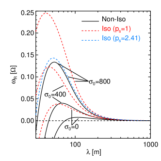
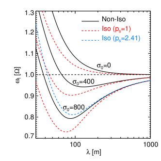
Figure 1: Theoretical linear growth rates (left) and oscillation frequencies (right) of overstable waves for ground state surface mass densities $\sigma_{0}=0,400$ and $800\,\text{kg}\,\text{m}^{-2}$. Parameters correspond to an optical depth of $\tau=1.5$ and $\Omega_{z}=3.6$ (see Section 3). All curves are calculated numerically from the exact Equation (16). The red isothermal curves are obtained in the limit $G_{T}\to\infty$ and $p_{s}=1$. For the blue isothermal curve (for $\sigma_{0}=800\,\text{kg}\,\text{m}^{-2}$) in each panel the value $p_{s}=2.41$ is used.

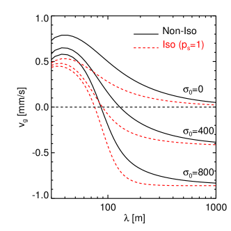
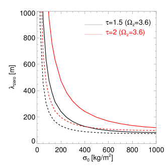
Figure 2: The left panel displays linear group velocities (23) of overstable waves for different ground state surface mass densities $\sigma_{0}$ (expressed in units $\,\text{kg}\,\text{m}^{-2}$). In the case of a non-zero self-gravity the oscillation frequency possesses a minimum at a certain wavelength, where the group velocity changes direction. This wavelength (right panel) decreases with increasing $\sigma_{0}$. The dashed curves represent the isothermal model ($G_{T}\to\infty$ and $p_{s}=1$). Parameters correspond to an optical depth of $\tau=1.5$ and $\Omega_{z}=3.6$ (see Section 3).

3 Hydrodynamic Parameters

The hydrodynamic model introduced in the previous section contains free parameters and transport coefficients which must be specified before equations (1) can be integrated. Sets of parameters were derived by Salo et al., (2001) from N-body simulations which were conducted for Saturnocentric distance $10^{5}\,\text{km}$ and $\Omega=1.95\cdot 10^{-4}\,\text{s}^{-1}$, using the Bridges et al., (1984) velocity- dependent coefficient of restitution and a particle radius of one meter. Self-gravity was approximated by an enhancement of the vertical frequency of oscillations, $\Omega_{z}/\Omega>1$, a method introduced by Wisdom and Tremaine, (1988). Because we neglect the effects of direct particle-particle gravity, these sets of parameters can in principle be used directly for our hydrodynamic integrations.

Note that the parameter $\Omega_{z}$ does not directly enter the hydrodynamic model. It affects indirectly through the altered transport coefficients. The enhancement of $\Omega_{z}$ has the effect of increasing the overall collision frequency, as self-consistent vertical gravity would do, which promotes viscous overstability. Throughout this paper we express values of $\Omega_{z}$ scaled with the Keplerian frequency $\Omega$. The collective radial gravity [Equation (2)] used in our model does not induce any changes in the transport properties of the ground state ring. This will be different if true gravitational encounters between individual particles are taken into account.

It must be kept in mind that the transport coefficients from Salo et al., (2001) are determined for a pre-specified parameterization of these quantities and their dependence on density and temperature [Equations (8)-(11)]. This parameterization is not unique and at this point it is not even clear if the particular form provided by equations (8)-(11) is well suited to follow the development into the nonlinear regime. The coefficients were determined in simulations from small amplitude perturbations of the ring ground state (Salo et al., (2001)), for which they are assumed to be representative. In the nonlinear regime, which we investigate in this study, we may therefore expect deviations of the hydrodynamical model from the results of the N-body simulations that arise from this problem.

In Table 3 we list the sets of parameters that are used for the hydrodynamic models in this paper. The columns specify the optical depths for which the parameters are valid. The parameter sets for $\tau=1.5$ and $\tau=2$ with $\Omega_{z}=3.6$ are highlighted with the labels $\tau_{15}$ and $\tau_{20}$, to which we will refer in the following. The last column, labeled $st99$, gives parameters which were used in the hydrodynamical model by Schmit and Tscharnuter, (1999). These parameters are based on the assumption that the ground state velocity dispersion takes the value $c_{0}=2\,\text{mm}\,\text{s}^{-1}$, which corresponds to a vertical ring thickness of $H\approx 10\,\text{m}$ by adopting the dilute estimate $H=c_{0}/\Omega$. The viscosity in this parameter set was then estimated by assuming an optical depth $\tau\sim 1$ and using the relation $\nu\sim 0.26\,(c_{0}^{2}/\Omega)\,\tau^{1.26}$, found by Wisdom and Tremaine, (1988). We use these parameters only to test our numerical scheme in the isothermal limit (Section 4.1.3). The rows of the table specify the factor of vertical frequency enhancement that was used by Salo et al., (2001) to determine the parameters, followed by the ground state effective velocity dispersion, the kinematic shear viscosity, the kinematic heat conductivity, and the granular temperature.

In Table 3 we provide a list of symbols with their numerical values used or, respectively, the characteristic scales which were employed to express our model in dimensionless form.

tableList of Symbols and their Scalings Quantity Scaling Value $c_{0}=\sqrt{\frac{p_{0}}{\sigma_{0}}}$ (effective velocity dispersion) $Q_{0}=\frac{\Omega c_{0}}{\pi G\sigma_{0}}$ (ground state Toomre-parameter) $G$ (gravitational constant) $6.67\cdot 10^{-11}\,\text{m}^{3}\,\text{kg}^{-1}\text{s}^{-2}$ $M_{S}$ (Saturn’s mass) $5.69\cdot 10^{26}\,\text{kg}$ $\Omega$ (orbital frequency at $r=10^{5}\,\text{km}$) $1.948\cdot 10^{-4}\,\text{s}^{-1}$ $x$ (radial coordinate) $c_{0}\,\Omega^{-1}$ $t$ (time) $\Omega^{-1}$ $k$ (wavenumber) $c_{0}^{-1}\,\Omega$ $\omega$ (complex wave frequency) $\Omega$ $\sigma$ (surface mass density) $\sigma_{0}$ $u$, $v$ (planar velocity components ) $c_{0}$ $T$ (temperature) $c_{0}^{2}$ $F_{\kappa}$ (heat flux) $\sigma_{0}\,c_{0}^{3}$ $\phi$ (self-gravity potential) $c_{0}^{2}$ $p$ (isotropic pressure) $\sigma_{0}\,c_{0}^{2}$ $\eta$ (dyn. shear viscosity) $\sigma_{0}\,c_{0}^{2}\,\Omega^{-1}$ $\kappa$ (dyn. heat conductivity) $\sigma_{0}\,c_{0}^{2}\,\Omega^{-1}$ $\Gamma$ (collisional cooling function) $\sigma_{0}\,c_{0}^{2}\,\Omega$ $\hat{P}$ (pressure tensor) $\sigma_{0}\,c_{0}^{2}$ $\hat{C}$ (velocity dispersion tensor) $c_{0}^{2}$ $\hat{S}$ (rate of strain tensor) $\Omega$

tableHydrodynamic Parameters $\tau=1$ $\tau=1.5\,(\tau_{15})$ $\tau=2.0\,(\tau_{20})$ $\tau=1.5$ $\tau=2.0$ $st99$ $\Omega_{z}\,[\Omega]$ 3.6 3.6 3.6 2.0 2.0 3.6 $c_{0}$ [$10^{-3}\,\text{m}\text{s}^{-1}$] 0.64 0.86 1.06 0.60 0.71 2.0 $\nu_{0}$ [$10^{-3}\,\text{m}^{2}\text{s}^{-1}$] 0.75 1.30 1.86 0.65 0.90 5.39 $\kappa_{0}$ [$10^{-3}\,\text{m}^{2}\text{s}^{-1}$] 3.14 5.38 7.61 2.78 3.53 - $T_{0}$ [$10^{-8}\,\text{m}^{2}\text{s}^{-2}$] 6.56 6.72 7.22 6.19 6.18 - $\gamma$ 2.14 1.99 2.12 2.06 1.99 1 $\beta$ 1.15 1.19 1.55 1.06 1.16 1.26 $n_{T}$ -0.13 -0.10 0.08 -0.12 -0.10 - $p_{s}$ 2.19 2.41 2.72 2.11 2.26 - $p_{T}$ 0.22 0.15 0.18 0.28 0.28 - $G_{s}$ 2.17 2.19 2.54 2.06 2.16 - $G_{T}$ 0.62 0.57 0.67 0.61 0.64 - $F_{2}$ -0.28 -0.28 0.08 -0.26 -0.28 - $F_{3}$ -0.35 -0.26 -0.48 -0.49 -0.48 -

4 Numerical Methods

4.1 Hydrodynamic Scheme

4.1.1 Discretization Technique

For numerical solution of the full nonlinear system (1) we bring these equations into flux-conservative form by defining

$$\mathbf{U}=\begin{pmatrix}\sigma\\ \sigma u\\ \sigma v\\ e\end{pmatrix}$$ (24)

with the energy density

$$e\equiv\sigma\left(\frac{1}{2}u^{2}+\frac{3}{2}T\right).$$ (25)

The two terms describe the radial kinetic and internal energy densities, respectively. By using these quantities the Equations (1) are equivalent to

$$\partial_{t}\mathbf{U}=-\partial_{x}\mathbf{F}+\mathbf{S}.$$ (26)

In this equation we define the flux vector

$$\mathbf{F}=\begin{pmatrix}\sigma u\\ \sigma u^{2}+p\\ \sigma uv\\ u\left(e+p\right)\end{pmatrix}$$ (27)

and the source term

$$\mathbf{S}=\begin{pmatrix}0\\ 2\Omega\sigma v-\sigma\partial_{x}\phi+\partial_{x}\Pi_{xx}\\ -\frac{1}{2}\Omega\sigma u+\partial_{x}\Pi_{xy}\\ 2\Omega\sigma uv+\hat{\Pi}:\mathbf{\nabla}\mathbf{u}-\Gamma-\partial_{x}F_{\kappa}-\sigma u\,\partial_{x}\phi+u\,\partial_{x}\Pi_{xx}\end{pmatrix}$$

where

$$\Pi_{kl}=p\delta_{kl}-P_{kl}$$

denotes the viscous stress tensor.

We solve the system (26) with a conservative finite difference method on a uniform mesh with nodes $x_{j}$, where $j=1,2,\ldots,n$, with grid spacing $h=x_{j+1}-x_{j}$. The spatial derivatives of the stress tensor components and the heat flux in $\mathbf{S}$ are evaluated with simple central discretizations of at least 6th order accuracy. The treatment of the radial self-gravity force $\partial_{x}\phi$ is described in the following section.

Since the solutions of Equations (1) are typically smooth structures, possibly interspersed with discontinuities (LO2010), a computation of the flux term is required which is highly accurate in the smooth regions while being able to resolve discontinuities without generating spurious oscillations. The popular Total Variation Diminishing (TVD) schemes are not suitable to distinguish an extremum from a discontinuity, which, in our case, would result in a loss of accuracy for large parts of the numerical solution, as we typically expect traveling periodic wave structures.

In order to discretize the flux term we follow Shu and Osher, (1988) and write

$$\partial_{x}\mathbf{F}\left(x_{j}\right)=\frac{\mathbf{f}_{j+1/2}-\mathbf{f}_{j-1/2}}{h},$$ (28)

where we introduce the “numerical flux function” $\mathbf{f}$ and where the subscripts $j\pm 1/2$ denote evaluation at the half nodes $x_{j}\pm h/2$. Equation (28) holds exactly if $\mathbf{f}$ is defined through

$$\mathbf{F}(x_{j})=\frac{1}{h}\int_{x_{j-1/2}}^{x_{j+1/2}}\mathbf{f}(\xi)\mathrm{d}\xi.$$ (29)

Our conservative scheme is then formulated by approximating the interface values between two neighboring cells of the mesh, $\mathbf{f}_{j+1/2}$ and $\mathbf{f}_{j-1/2}$, by using relation (29) and the fact that the cell averages $\mathbf{F}(x_{j})$ are known for all $j$, since these are the values of the physical flux (27) at the nodes $x_{j}$.

The basic procedure is as follows (e.g. Shu, (2009)). One defines the primitive function of $\mathbf{f}(x)$ by

$$\mathbf{p_{f}}(x)=\int_{x_{0}}^{x}\mathbf{f}(\xi)\mathrm{d}\xi,$$ (30)

with arbitrary lower limit $x_{0}$. The function $\mathbf{p_{f}}(x)$ is then approximated by a Lagrange-polynomial of order $2r-1$ which interpolates through the $2r$ (with integer $r\geq 2$) data points $[x_{i+1/2},\mathbf{p_{f}}(x_{i+1/2})]$ with $i=j-r,j-r+1,\ldots,j+r-1$. Here

$$\begin{split}\mathbf{p_{f}}(x_{i+1/2})&=\int_{x_{0}}^{x_{i}+h/2}f(\xi)\mathrm{d}\xi\\ \quad&=\hat{C}+\sum_{l=j-r}^{i}\int_{x_{l}-h/2}^{x_{l}+h/2}f(\xi)\mathrm{d}\xi\\ \quad&=\hat{C}+\sum_{l=j-r}^{i}h\,\mathbf{F}(x_{l})\end{split}$$ (31)

are the interface values of the primitive function. The constant $\hat{C}$ depends on the choice of $x_{0}$. Differentiation of the interpolating polynomial for $\mathbf{p_{f}}(x)$ with respect to $x$ then yields a polynomial of order $2r-2$ which can be used to obtain approximations $\mathbf{\hat{f}}_{j-1/2}$, $\mathbf{\hat{f}}_{j+1/2}$ of the exact numerical flux values in Equation (28). The hats indicate that these values fulfill (28) up to an error, which depends on the degree of the interpolating polynomial.

In order to handle discontinuities, we utilize the MP5 algorithm (Suresh and Huynh, (1997)) which applies monotonicity preserving bounds on the interface values $\mathbf{\hat{f}}_{j-1/2}$, $\mathbf{\hat{f}}_{j+1/2}$ which are obtained with the method described above from a 6-point stencil ($r=3)$. This scheme is uniformly 5th order accurate, such that

$$\partial_{x}\mathbf{F}\left(x_{j}\right)=\frac{\mathbf{\hat{f}}_{j+1/2}-\mathbf{\hat{f}}_{j-1/2}}{h}+\mathcal{O}(h^{5}),$$

anywhere, except for discontinuities.

Time integration is performed with a 5-stage 4th order accurate TVD Runge-Kutta method (SSPRK(5,4)) developed in Ruuth, (2006). The reason for using a strong stability preserving (SSP) time discretization instead of a regular variant is that the computational costs remain the same while these methods can improve stability when solving hyperbolic conservation laws (Gottlieb et al., (2001)).

Attempting to conduct a stability analysis of only the linearized version of above equations leads to an eigenvalue problem which cannot be solved analytically. As a simple criterion for the time steps we take as a guide the time step restriction which arises for a simple one dimensional advection-diffusion problem

$$\partial_{t}u+\lambda\partial_{x}u=\nu\partial_{x}^{2}u,$$

integrated with a first order Euler forward method (the building block of any multi-stage SSP Runge-Kutta scheme) and second order central differences for the discretization of the spatial derivatives. This restriction reads

$$\Delta t\leq\text{min}\left(\frac{\Delta x^{2}}{2\nu},\frac{2\nu}{\lambda^{2}}\right)$$ (32)

where $\lambda$ is identified with the maximal eigenvalue of the Jacobian

$$\hat{A}=\frac{\partial\mathbf{F}(\mathbf{U})}{\partial\mathbf{U}}$$ (33)

of the actual system of equations (26) for the whole grid. Since we are using higher order spatial discretizations and since we are solving a system of equations we multiply this time step restriction in practice by a factor $0<f_{t}<1$ , as was done in LO2010. We use $f_{t}=0.1$ in most cases. The resulting typical time steps lie in the range of $10^{-2}-10^{-4}$ orbital periods, depending on the grid resolution, the used parameter set and the evolutionary stage of the integration. The scaled (Table 3) eigenvalues of the non-isothermal Jacobian (33) read

$$\begin{split}\lambda_{(1/2)}&=u,\\ \lambda_{(3/4)}&=u\pm\frac{3^{(-p_{T})}}{\sigma(-2e+\sigma u^{2})}\left[T_{0}\,\sigma^{(2+p_{s})}\left(\frac{2e-\sigma u^{2}}{\sigma T_{0}}\right)^{(1+p_{T})}\right.\\ \quad&\left.\left(3^{(p_{T})}\,p_{s}\,(2e-\sigma u^{2})+2p_{T}\,\sigma^{(p_{s})}\left(\frac{2e-\sigma u^{2}}{\sigma T_{0}}\right)^{(p_{T})}\right)\right]^{1/2}.\end{split}$$ (34)

In the isothermal limit with the ideal gas relation of state, these reduce to the three eigenvalues

$$\begin{split}\lambda_{1}&=u,\\ \lambda_{(2/3)}&=u\pm 1.\end{split}$$ (35)

The homogeneous version of Equation (26), i.e. the case $\mathbf{S}=0$, is a hyperbolic system of partial differential equations such that the Jacobian possesses a complete set of independent eigenvectors with only real eigenvalues [(34), (35)]. Its (eigen)solutions follow characteristics. This is accounted for by a correct upwinding of the numerical solution through a splitting of the physical flux (27) prior to the reconstruction of the numerical flux $\mathbf{f}$. The splitting is performed such that

$$\mathbf{F}(\mathbf{U})=\mathbf{F}^{+}(\mathbf{U})+\mathbf{F}^{-}(\mathbf{U})$$ (36)

with

$$\hat{A}^{+}\equiv\frac{\partial\mathbf{F}^{+}(\mathbf{U})}{\partial\mathbf{U}}\geq 0\hskip 8.5359pt\text{and}\hskip 8.5359pt\hat{A}^{-}\equiv\frac{\partial\mathbf{F}^{-}(\mathbf{U})}{\partial\mathbf{U}}\leq 0.$$ (37)

The notation means that $\hat{A}^{+}$ has only non-negative eigenvalues whereas $\hat{A}^{-}$ has only non-positive eigenvalues. In order to obtain correct upwinding for a general splitting (36), (37), $\mathbf{f}^{+}_{j+1/2}$ and $\mathbf{f}^{-}_{j+1/2}$ are reconstructed from $2r$ data points $[x_{i+1/2},\mathbf{F}(x_{i+1/2})]$ with $i=j-r,j-r+1,\ldots,j+r-1$ and $i=j-r+1,j-r+2,\ldots,j+r$, respectively [cf. Equation  (31)]. In this paper we apply the Liou-Steffen splitting (Liou and Steffen, (1993)).

All hydrodynamic integrations are performed by assuming periodic boundary conditions in a radial domain whose size we denote by $L_{x}$. This means that each component $U_{i}$ (i=1,2,3,4) of the numerical solution vector (24) at any time possesses the Fourier representation

$$U_{i}=\sum_{m=0}^{n/2-1}\hat{U}_{i}^{m}\cos \left(k_{m}\,x+\varphi_{m}\right)$$ (38)

with real-valued Fourier amplitude $\hat{U}_{i}^{m}$, wavenumber $k_{m}=m\,2\pi/L_{x}$ and phase $\varphi_{m}$ of each mode $m$.

For later use we also define the mean kinetic energy density within the computational domain as

$$e_{kin}=\frac{1}{L_{x}}\int\limits_{[L_{x}]}\mathrm{d}x\,\frac{1}{2}\sigma\left(u^{2}+v^{2}\right).$$ (39)

4.1.2 Implementing Radial Self-Gravity

The implementation of self-gravity forces in a hydrodynamic simulation is in general a difficulty of its own. Fortunately, the wave structures we study here can be treated as purely radial to a good approximation, so that the computation of the self-gravity is greatly simplified.

We neglect curvature and describe the axisymmetric density pattern as a collection of straight wires of infinite azimuthal extent. A wire at radial location $x$ has a surface mass density

$$\sigma(x)=\frac{1}{h}\frac{\mathrm{d}M}{\mathrm{d}y}$$ (40)

where $\mathrm{d}M/\mathrm{d}y=const.$ denotes the mass of the wire per unit length in $y$-direction and $h$ is its radial size. From this follows that a cell which has a radial distance $x$ from a reference location generates a radially directed gravitional force:

$$\Delta f^{disk}=Gh\sigma_{0}\int\limits_{-\infty}^{\infty}\mathrm{d}y\,s(x)\,\frac{x}{\left(x^{2}+y^{2}\right)^{3/2}}=2Gh\sigma_{0}\frac{x}{|x|^{2}}s\left(x\right)$$ (41)

where we defined $s(x)=\sigma(x)/\sigma_{0}$. This model applied to our scheme then yields a self-gravity force at grid point $j$:

$$f^{disk}_{j}=-2Gh\sigma_{0}\sum_{l=1,l\neq j}^{n}s(x_{l})\,\frac{x_{j}-x_{l}}{|x_{j}-x_{l}|^{2}}.$$ (42)

As it stands, relation (42) neglects the force generated by mass contained in the bin $j$ itself, which is given by

$$\Delta f^{disk}(0)=2G\sigma_{0}\left[\partial_{x}s(0)\,h+\mathcal{O}\left(h^{3}\right)\right].$$ (43)

Evaluating Equation (42) for the whole grid by direct summation would involve of the order of $n^{2}$ operations, where the number of grid points can get as large as $n\sim 10^{4}$. However, using the periodicity of $s(x_{l})$, the sum (42) can be written as a convolution

$$f^{disk}_{j}=\sum_{l=-n}^{n-1}s_{l}\,f^{kern}_{j-l}$$ (44)

of $s_{l}=s(x_{l})$. The force kernel reads

$$f^{kern}_{j-l}=-2Gh\sigma_{0}\frac{x_{j}-x_{l}}{|x_{j}-x_{l}|^{2}}.$$ (45)

Equation (44) can be solved efficiently with a FFT method, which needs only of the order of $n\log n$ steps. The discrete Fourier convolution theorem states that (see for example Binney and Tremaine, (1987)) the Fourier transforms are related as

$$\mathcal{F}_{k}\left(f^{disk}\right)=\mathcal{F}_{k}\left(s\right)\cdot\mathcal{F}_{k}\left(f^{kern}\right)$$ (46)

and therefore the self-gravity force is obtained as a back transformation

$$f^{disk}_{j}=\mathcal{F}_{j}^{-1}\left[\mathcal{F}_{k}\left(s\right)\cdot\mathcal{F}_{k}\left(f^{kern}\right)\right].$$ (47)

Equations (46) and (47) can be solved efficiently by using a FFT. In our simulations we will exclusively make use of periodic boundaries, so that the FFT is directly applicable without the need to pad extended arrays with zero’s (Binney and Tremaine, (1987)). The self-gravity force (42) neglects far field contributions (with $|x_{j}-x_{l}|>L_{x}$), since the kernel (45) ranges over a limited region. This restriction can be overcome by adding contributions from additional neighboring replicas of the original density field to the kernel.

4.1.3 Tests

Before we apply our hydrodynamical integration scheme to viscous overstability in planetary rings we perform several tests. Here we resort to established results from linear theory, checking the accuracy of our scheme by measuring growth rates and oscillation frequencies of linear overstable modes (14). These should agree with values obtained with numerical solution of (16). In these test integrations the calculation of self-gravity is performed with the corrective term (43), as well as an extension of the self-gravity kernel (45) with 5 adjacent replica’s on each side of the computational domain. For both the isothermal and the non-isothermal schemes we use the $\tau_{15}$-parameters (Table 3). Surface mass densities $\sigma_{0}=0$, $\sigma_{0}=350\,\text{kg}\,\text{m}^{-2}$ and $\sigma_{0}=600\,\text{kg}\,\text{m}^{-2}$ are adopted.

To measure linear growth rates, we use a computational domain with $L_{x}=1\,\text{km}$ and seed all modes down to about $\lambda=30\,\text{m}$ at once, with small amplitudes. This initial state is then integrated for about 15 orbital periods. To obtain the growth rate of a mode $m$, we perform a linear fit to the corresponding Fourier-amplitude $\log(\hat{U}_{i}^{m})$ [cf. (38)].

Linear frequencies are obtained from short integrations (up to about 30 orbital periods), where we follow the evolution of a single seeded small amplitude mode in a domain of radial size $L_{x}=\lambda$. The oscillation frequencies are measured by analyzing the time evolution of the radial velocity field of a linear overstable mode at a fixed radial location with the Lomb-periodogram (Press et al., (1992)) to obtain the dominant frequency.

During these integrations, we make sure that amplitudes of all other (non-seeded) modes remain less than about 0.1 $\%$ of the amplitude of the seeded mode. For convenience we use as a seed the eigensolutions of the isothermal hydrodynamic equations, which are available in analytical form (Schmidt et al., (2001)).

For brevity, we present here only the results for the non-isothermal model, the isothermal case being very similar. Figure 3 displays measured growth rates and oscillation frequencies. With a grid resolution $h=1\,\text{m}$ the error of the computed growth rates and oscillation frequencies is less than one percent on all relevant length scales. Neglecting the above mentioned corrections to the computation of self-gravity leads to mild drops of the growth rates, as well as mild enhancements of the oscillation frequencies, however, being less than 5 percent on all relevant length scales. We do not include these corrections in our integrations of the nonlinear evolution of overstability, because they do not affect the outcome in a significant manner. The neglect of the finite bin size correction can be interpreted as a smoothing of structures on very short length scales. Especially the kernel extension is not necessary since the box sizes are in all integrations presented in the following sections chosen large enough to comprise many wavelengths of each relevant mode.

Figure 3: Non-isothermal hydrodynamic linear growth rates (left panel) and oscillation frequencies (right panel) of overstable modes with the $\tau_{15}$-parameters. Symbols denote the values obtained with the flux-conservative integration scheme and the lines represent the theoretical curves obtained with numerical solution of (16).

4.2 N-Body Simulations

We adopt the local simulation method (Wisdom and Tremaine, (1988)) which was used by Salo et al., (2001) (see also Salo, (1992) and Salo, (1995)). Thus, we simulate $N_{p}$ particles contained in a small rectangular region, co-moving with the mean Keplerian angular frequency $\Omega=\sqrt{GM_{S}/r^{3}}$ at distance $r=10^{5}\,\text{km}$ from the planet. The simulation region has dimensions $L_{x}\times L_{y}$ in a cartesian coordinate system $[x,y,z]$ where the $x$-axis points radially outward and the $y$-axis is directed along the orbital motion. In radial and azimuthal direction we apply periodic boundary conditions. Particles crossing the radial box boundary re-enter with appropriately modified velocities to account for the shear.

Particles are identical, smooth, spin-less spheres, with radius $R_{p}=1\,\text{m}$. Furthermore, to describe collisional energy loss in simulations, we use either a constant normal coefficient of restitution $\epsilon=0.5$, or the Bridges et al., (1984) collision law

$$\epsilon_{b}(v_{n})=\left(\frac{v_{n}}{v_{c}}\right)^{-0.234}$$ (48)

with $v_{n}$ being the normal component of the relative velocity vector of two impacting particles and the scale parameter $v_{c}=0.077\,\text{mm}\,\text{s}^{-1}$. This relation was used in the simulations described in Salo et al., (2001). The constant $\epsilon=0.5$ leads to a system which mimicks very well the cool, flattened ring state resulting from $\epsilon_{b}(v_{n})$ and for our purposes the two cases yield practically the same results. Particle collisions are modeled with the same visco-elastic impact model that was originally devised by Dilley, (1993) to parameterize measurements of elasticity (see Salo, (1995)).

The motion of each particle is described with the Hill-equations

$$\begin{split}\ddot{x}-2\Omega\dot{y}+\left(\kappa^{2}-4\Omega^{2}\right)x&=F_{x}+F^{g}(x)\\ \ddot{y}+2\Omega\dot{x}&=F_{y}\\ \ddot{z}+\Omega_{z}^{2}z&=F_{z}\end{split}$$ (49)

where $\kappa$ is the epicyclic frequency which equals $\Omega$ in this study, because we neglect effects from the oblateness of the planet. Furthermore, $F_{x}$, $F_{y}$, $F_{z}$ describe forces per unit mass due to particle impacts and $F^{g}(x)$ denotes the radial collective self-gravity force per unit mass, which we discuss in the next section. Note that the vertical frequency $\Omega_{z}$ is enhanced compared to $\Omega$, mimicking the effect of vertical self-gravity (Wisdom and Tremaine, (1988)). Parameters used in the N-body simulations are given in Table 4.2.

tableN-Body Simulation Parameters of Large-Scale Runs

$\tau$	$1.5$	$1.5$	$1.5$	$2$
$\Omega_{z}\,[\Omega]$	3.6	3.6	2	3.6
$\epsilon$	$\epsilon_{b}$	0.5	$\epsilon_{b}$	0.5
$L_{x}$	$2\,\text{km}$	$5\,\text{km}$	$2\,\text{km}$	$5\,\text{km}$
$L_{y}$	$10\,\text{m}$	$31.41\,\text{m}$	$10\,\text{m}$	$25.14\,\text{m}$
$N_{p}$	9,550	75,000	9,550	80,000
$R_{p}$	1m
$\sigma_{0}$	free parameter

4.2.1 Treatment of Self-Gravity in N-Body Simulations

It is well known from theoretical treatments and from simulations that the vertical component of self-gravity leads to a flattening of the ring, thereby increasing the collision frequency of the ring particles. The high collision frequency in principle promotes viscous overstability, as it increases the relative contribution of nonlocal momentum transport, resulting in an effective shear viscosity which increases steeply with increasing optical depth.

The effects of the planar components of self-gravity on instability mechanisms such as the viscous overstability are less well understood. According to kinetic treatments (e.g. Shu and Stewart, (1985)) and simulations (e.g. Salo, (1995)), self-gravitational encounters contribute to the local viscosity of the system, transferring energy from systematic motion to random motions. This is efficient if the velocity dispersion is smaller than the mutual two-body escape speed $v_{esc}=\sqrt{2Gm_{0}/R_{p}}$ of ring particles with mass $m_{0}$. Therefore, $v_{esc}$ becomes a lower limit for the velocity dispersion in self-gravitating particulate systems. Theoretically, in a dilute inviscid disk, the planar self-gravity can lead to local instability of axisymmetric modes if the radial component of the velocity dispersion fulfills $c_{r}<c_{crit}=3.36G\sigma/\kappa$ (Toomre, (1964)). In terms of the Toomre-parameter this threshold reads $Q<1$. Nevertheless, in realistic self-gravitating simulations of Saturn’s dense rings it is found (Salo, (1992, 1995)) that $Q$ often adjusts to values around 2. The system is found to be no longer uniform and self-gravity wakes form and dissolve on orbital timescales. These non-axisymmetric structures contribute to the angular momentum transport through gravitational torques as well as through their systematic motion. It turns out that in the presence of wakes the nonlocal viscosity becomes unimportant, compared to the roughly equal contributions from the (strongly enhanced) local and gravitational viscosity (Daisaka et al., (2001)). The wakes heat up the particle system, establishing a steady state Toomre-parameter above 1, depending on the precise particle properties, like $\epsilon$, internal density and particle radius.

In this study we neglect the direct gravitational interactions during particle encounters. Consequently, the simulated ring states lack the related heating processes, which results in significantly lower (ground state) velocity dispersions. But most importantly, since wake structures do not appear, the ground state is homogeneous and we can use the transport coefficients determined by Salo et al., (2001) when comparing to our hydrodynamic scheme (section 4.1).

In the N-body simulations presented in this paper two aspects of self-gravity are taken into account. First, vertical self-gravity is approximated by an artificially increased frequency of vertical oscillations in the Hill-equations of motion (49), resulting in the effects described above. We adopt for most simulations the factor $\Omega_{z}=3.6$, which was originally introduced by Wisdom and Tremaine, (1988), and which was later also used by Rein and Latter, (2013). Furthermore, the transport coefficients used in the hydrodynamical model in LO2009 and LO2010 were obtained from N-Body simulations with the same $\Omega_{z}=3.6$ (Salo et al., (2001)). In this approximation the vertical self-gravity is assumed to be generated by a homogeneous slab of material with vertical thickness $H$ and with ($z$-independent) volume density $\rho=\sigma_{0}/H$ so that vertical integration of the Poisson equation results in

$$\partial_{z}\phi(z)=\frac{4\pi G\sigma_{0}}{H}z,$$ (50)

where $|z|\leq H/2$, i.e. within the homogeneous slab. Combined with the planet’s vertical force this results in a total vertical force

$$F_{z}(z)=-\left(1+\frac{4\pi G\sigma_{0}}{\Omega^{2}\,H}\right)\Omega^{2}\,z\equiv-\Omega_{z}^{2}\,z,$$ (51)

defining thereby the (scaled) effective vertical frequency $\Omega_{z}$. Note that the chosen value $\Omega_{z}/\Omega=3.6$ is larger than the vertical enhancement in rings. It is chosen mainly to enable a direct comparison with the aforementioned studies.

Moreover, following Salo and Schmidt, (2010), we model the radial component of self-gravity in a manner which is similar to the method used in our hydrodynamic scheme (section 4.1.2). The force calculation is based on a radial Fourier-decomposition of the tangentially averaged surface density

$$\sigma(x)=\sigma_{0}\,\left[1+\sum_{m=1}^{m_{max}}A_{m}\cos \left(k_{m}\,x+\varphi_{m}\right)\right]$$ (52)

with wavenumbers $k_{m}=m\,2\pi/L_{x}$ and where $A_{m}$ and $\varphi_{m}$ denote the amplitude and phase of the corresponding Fourier mode. The cutoff $m_{max}$ is to be chosen sufficiently high (typically a few hundreds) in order to avoid aliasing effects. Each of the $m_{max}$ plane waves in (52) contributes to the radial self-gravity potential through relation (15), i.e.

$$\phi_{m}\left(x\right)=\frac{2\pi G\sigma_{0}}{k_{m}}\,A_{m}\cos \left(k_{m}\,x+\varphi_{m}\right).$$ (53)

The total radial self-gravity force per unit mass then reads

$$F^{g}(x)=-2\pi G\sigma_{0}\,\sum_{m=1}^{m_{max}}A_{m}\sin \left(k_{m}\,x+\varphi_{m}\right).$$ (54)

One notes that the ground state surface density $\sigma_{0}$ is now a free model parameter, as the simulated particles are otherwise massless. The tangential component of self-gravity is not considered since we assume that the ring retains azimuthal symmetry. Both, this method and the self-gravity implementation applied in the hydrodynamic scheme (Section 4.1.2) neglect curvature, consistent with the hydrodynamic model presented in Section 2. From a theoretical point of view the mode calculation (54) is more accurate than the straight wire model (42) since it automatically assumes infinite extent of waves, whereas the kernel (45) ranges over a limited region, thus neglecting far distance contributions. As stated in Section 4.1.2 this restriction can in principle be overcome by adding contributions from additional neighboring replicas of the original density field to the kernel.

4.2.2 Growth Rates and Oscillation Frequencies of Overstable Modes in the Linear Regime

In the determination of linear growth rates from N-body simulations we seed one single mode with a small initial amplitude and a wavelength $L_{x}/m$ ($m$ is the mode number). Only this mode is taken into account in the calculation of radial self-gravity. As in the hydrodynamic measurements (Section 4.1.3) the growth rate is computed from a linear fit to the time evolution of the corresponding Fourier amplitude, while the oscillation frequency is obtained with the Lomb normalized periodogram. Care is taken to use a time interval during which the oscillation amplitude remains small, typically about 20 orbital periods. The box size used in these simulations is $L_{x}=1\,\text{km}$, and the measured modes cover $m=1-25$ (down to 40 meters).

Figure 4 shows the linear growth rates in simulations with different optical depths $\tau$, along with theoretical curves resulting from the non-isothermal model. We find that for $\sigma_{0}=0$ the growth rates of the hydrodynamic model and the N-Body simulations match reasonably well for all optical depths (cf. Schmidt et al., (2001)). With the higher optical depth $\tau=2$ we obtain good agreement also for the moderate surface density $\sigma_{0}=350\,\text{kg}\text{m}^{-2}$. For smaller optical depths though, there develops discrepancy with increasing $\sigma_{0}$. From Figure 4 follows that, contrary to the hydrodynamic prediction, decreasing the optical depth from $\tau=2$ towards $\tau=1$ does not lead to an overall increase of the growth rates, but merely produces a shift toward shorter wavelengths.

In Figure 5 we present results for growth rates and oscillation frequencies for fixed optical depth $\tau=1.5$ and $\Omega_{z}=3.6$ but varying surface density $\sigma_{0}$. The solid curves represent the non-isothermal model, computed from Equation (16). While the hydrodynamic model overestimates the growth rates, it tends to underestimate the oscillation frequency. Overall, it provides a good match for modes of larger wavelength.

The deviations might to some extent arise from the vertical dynamics of the simulated particulate disk. Namely, vertical expansions of the disk will affect the isotropic pressure and the transport coefficients on the orbital timescale and this interferes with the growth of overstable modes. For the self-gravitating runs we observe a related vertical splashing of ring particles in the compressed phases of the oscillations (cf. Figure 16 and Figure 1 in Salo et al., (2001)) already during the linear growth phase. Splashing occurs since the ring flow is nearly incompressible (Borderies et al., (1985)).

The dashed curves in Figure 5 are non-isothermal model curves computed with a pressure coefficient $p_{s}$ [cf. Equation (8)] that was increased by 40 percent from its nominal value (Table 3). For clarity, we plot modified curves in both panels only for the three largest values of $\sigma_{0}$. This modification of a single parameter leads overall to a considerably better agreement with the results from N-body simulations in the linear regime. However, significant deviations remain in the nonlinear regime. This will be further discussed in Section 6.1 and Appendix B.2.

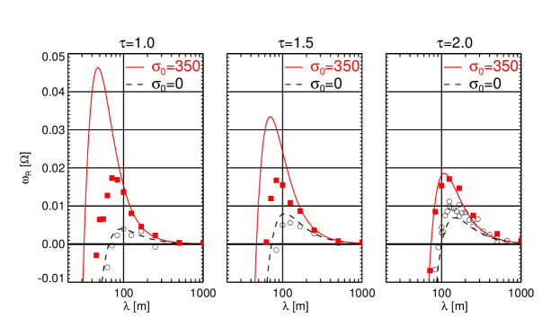
Figure 4: Growth rates of linear overstable modes from N-body simulations with different optical depths for $\Omega_{z}=3.6$. Filled squares correspond to $\sigma_{0}=350\,\text{kg}\,\text{m}^{-2}$ and open circles to $\sigma_{0}=0$. The curves represent the corresponding hydrodynamic predictions for which we used the parameter sets listed in Table 3.

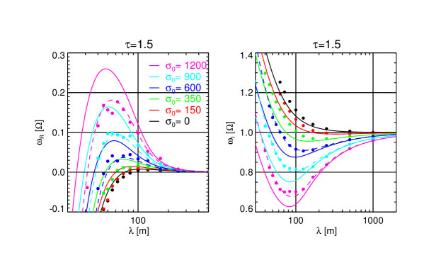
Figure 5: Linear growth rates (left) and oscillation frequencies (right) from N-body simulations with optical depth $\tau=1.5$ for various surface densities. Non-isothermal hydrodynamic model curves (solid) for the same surface densities $\sigma_{0}$ (units $\text{kg}\,\text{m}^{-2}$) are shown in the same color. The dashed curves result from the hydrodynamic model with an increased value of $p_{s}$ by $40\%$.

5 Results

We begin by presenting results of the hydrodynamic model in the limit of vanishing self-gravity in Section 5.1. Here we distinguish between the isothermal and non-isothermal cases. We perform a qualitative comparison to the hydrodynamic results of LO2010 and to the non-gravitating N-Body simulations of RL2013. In section 5.2 we present the hydrodynamic model with radial self-gravity. We restrict the description mainly to integrations with the vertical frequency $\Omega_{z}=3.6$ to facilitate the comparison with the aforementioned work. Our integrations with $\Omega_{z}=2$ behave qualitatively similar. The Section 5.3 is devoted to the results of our gravitating N-Body simulations and comparison to the hydrodynamic model.

5.1 Hydrodynamical Integrations Without Self-Gravity

5.1.1 Isothermal Model

Our isothermal model without self-gravity produces results very similar to those presented in LO2010.

Figure 6 shows snapshots of the hydrodynamic field quantities during two different stages of nonlinear evolution with the $\tau_{15}$-parameters. The seed for this integration is spectral white noise consisting of both left and right traveling, small amplitude waves. The left panel represents an intermediate state of the evolution in which the initial perturbations have already attained substantial amplitudes and different modes begin to interact with each other. The plots reveal the presence of a source/sink pair for traveling waves in the system. The source coincides with the density depletion near $x=4.5\,\text{km}$. At this location also the velocity amplitudes are small. The corresponding sink is less easy to locate. It reveals itself through a reversal in the shape of the radial velocity profile $u$ (across $x=-3\,\text{km}$), indicating that the two nonlinear traveling waves collide at this point. In the advanced wave state, displayed in the right panel, these structures have disappeared, leaving a unidirectional wave train which fills out the entire domain and which undergoes small amplitude and phase fluctuations.

Figure 7 shows for the same integration a stroboscopic space-time diagram, as well as the final power spectrum of the surface mass density field. In the space-time diagram lines of constant gray-shading indicate lines of constant phase of the wave structures. The term stroboscopic means that the diagram is plotted with a sampling rate of $1/\text{orbit}$ (see Appendix A). Source and sink structures are clearly visible in this diagram. The sources are the gray stripes which remain at nearly fixed locations, showing only small radial excursions. These are interconnected by the (less pronounced) sinks. We observe initially four source/sink pairs. The sources emit a complicated sequence of phase modulations, which are expected to travel with the corresponding group velocity for these wavelengths. It is also seen that the sinks wander in a stochastic manner towards the sources, resulting eventually in an annihilation of the two. One pair survives for about 7,000 orbits.

Following van Hecke et al., (1999), sources are active structures which send out waves, while sinks are locations where the waves meet and disappear. The distinction between sources and sinks in a space-time diagram is to be made according to the sign of the group velocity of the adjacent wave patches. The group velocity points away from sources and towards sinks. In the usual definition, sources and sinks are coherent structures which can appear in solutions of the complex coupled Ginzburg-Landau (CGL) equations. As outlined for instance in van Hecke et al., (1999), this applies to systems which undergo a supercritical Hopf-bifurcation from a homogeneous ground state into a traveling wave state (such as the viscously overstable fluid disk investigated here), where the interaction between counter-propagating waves is large enough so that these can suppress each other. Then the system can develop unidirectional wave patches, separated by (stable) sinks and sources. In some parameter regimes of the CGL equations, these structures can exhibit highly complex dynamics.

Once all sources and sinks have disappeared, the perturbations eventually develop into a single traveling wave mode which subsequently increases its wavelength through a so called staircase process (LO2010). The different stages of development are visible in the evolution of the kinetic energy density $e_{kin}$ (39), presented in Figure 8 (left panel: lower red curve marked $\tau_{15}$). This plot also shows the evolution of $e_{kin}$ of an initial white noise state with the $\tau_{20}$-parameters (upper red curve marked $\tau_{20}$). The remaining three black curves correspond to integrations of initial states consisting of a single mode ($\lambda=100\,\text{m}$) with the $\tau_{15}$, the $\tau_{20}$, as well as the $st99$-parameters.

The kinetic energy densities describing the integrations from white noise (the red curves) exhibit fluctuations during the intermediate stage of the evolution. These are caused by the presence of the source/sink structures (Figure 7, left panel), since the nonlinear waves connecting these structures undergo wavelength and amplitude fluctuation. In contrast, the systems which evolve from a $\lambda=100\,\text{m}$ mode do not exhibit source/sink pairs. This explains the lack of fluctuations in their kinetic energy curves (the three black curves).

Figure 8 (right panel) shows for these three integrations starting from the $\lambda=100\,\text{m}$ mode the evolution of the prevalent wavelength $\lambda_{p}$. This wavelength corresponds to the maximum of the power spectral density (cf. Figure 7, right panel), as a function of time. Nonlinear self-interactions of the wave train on the average result in a growth of $\lambda_{p}$, accompanied by strong fluctuations, until it eventually settles on a constant value. The final values of $\lambda_{p}$ are in good agreement with the wavelengths $\lambda_{st}$ found by LO2009, who have shown that all nonlinear wave trains with a wavelength larger than $\lambda_{st}$, are stable with respect to perturbations, while those with $\lambda<\lambda_{st}$ are not. This picture explains the observed growth of $\lambda_{p}$ towards these critical values, induced by small perturbations of the wave trains. It is, however, in principle possible that the system settles on a considerably larger wavelength or even on a set of multiple wavelengths, depending on the precise initial conditions. Values for $\lambda_{st}$, determined by LO2009 are given in the caption of Figure 8.

Figure 6: Hydrodynamic fields characterizing intermediate (t=4,000 ORB, left panel) and advanced states (t=20,000 ORB, right panel) of an isothermal integration with the $\tau_{15}$-parameters. Radial self-gravity is not included ($\sigma_{0}=0$).

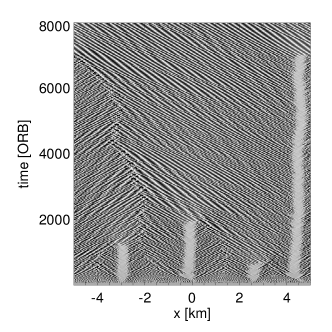
Figure 7: Stroboscopic space-time diagram (left panel) and final normalized power spectral density (PSD) of the surface mass density field (right panel) for the same integration as in Figure 6 with the $\tau_{15}$-parameters.

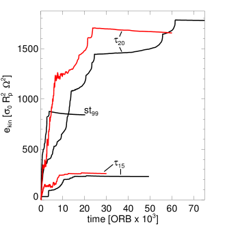
Figure 8: Left: Evolution of kinetic energy densities of hydrodynamic integrations in the isothermal model without self-gravity with the $\tau_{15}$, the $\tau_{20}$, and the $st99$-parameters (see Table 3). The initial states corresponding to the red curves are small amplitude spectral white noise, those corresponding to the black curves consist of a small amplitude wave with $\lambda=100\,\text{m}$. The red curve labeled $\tau_{15}$ is from the same integration as described in Figures 6 and 7. Right: Evolution of the prevalent wavelength corresponding to the three black curves in the left panel. The final values of $\lambda_{p}$ are in good agreement with the values $\lambda_{st}=233\,\text{m},455\,\text{m},\,659\,\text{m}$, computed for the same parameters by LO2009. In all integrations we used $L_{x}=10\,\text{km}$ with $h=2.5\,\text{m}$. Note that for the units of $e_{kin}$ we adopt $R_{p}=1\,\text{m}$ to compare with our N-Body simulations in Section 5.3.

We also perform a few integrations where we include a buffer-zone in the calculation region, i.e. a small radial sub-region where the density exponent of the viscosity in Equation (9) takes values $-1<\beta<\beta_{c}$. In such a region the condition for viscous overstability is not fulfilled so that the linear growth rate of overstable modes (21) is negative. Waves which travel into this region are consequently damped. This modification introduces an obstacle for traveling waves, a situation that might typically occur in Saturn’s rings when the background properties change. A buffer-zone leads in all considered cases to a state with one source and one sink structure, where the buffer-zone serves as the latter. The long term prevalent wavelengths in these integrations are concentrated around those wavelengths which we also find for the final traveling waves in the homogeneous boxes. Figure 9 displays the outcome of an isothermal integration with a buffer-zone.

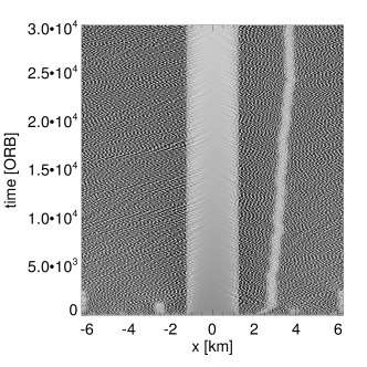
Figure 9: Isothermal integration with the $\tau_{15}$-parameters and $\sigma_{0}=0$ (no radial self-gravity) where a buffer-zone is included such that $\beta=-0.5$ in the radial domain $[-1.25\,\text{km};+1.25\,\text{km}]$. In this zone the hydrodynamic state is modified, so that overstable waves will damp (see text). Left and right panels show a stroboscopic space-time diagram and the final power spectrum, respectively.

5.1.2 Non-isothermal Model

The non-isothermal scheme in the limit of vanishing radial self-gravity produces results that agree reasonably well with the non self-gravitating N-body simulations presented in RL2013. Figures 10 and 11 describe an integration with the $\tau_{20}$-parameters. The initial state of the integration is spectral white noise with wavelengths down to $\lambda\sim 50\,\text{m}$. After complicated, disordered transient states, with strongly asymmetric sink and source structures, the system settles on a single traveling wave state.

For comparison, the final state wavelengths we find with the $\tau_{15}$ and $\tau_{20}$-parameters are about $\lambda=360\,\text{m}$ and $\lambda=570\,\text{m}$ (Figure 11, right panel), respectively. This is in good agreement with the final wavelength of the “fiducial run” from RL2013 with $\tau=1.64$ which is close to $\lambda=450\,\text{m}$. Overall, these results indicate a trend of increasing final state wavelength with increasing ground state optical depth, which was expected also by LO2009 on theoretical grounds.

The colliding waves penetrate each other over many wavelengths in the sink structures before they damp. In contrast, we find fairly narrow sink and source structures in the isothermal model (cf. Figure 7). RL2013 discussed the same discrepancy between the appearance of sources and sinks in their N-body simulations, compared to those in the isothermal hydrodynamic model of LO2010. They attributed it to the particulate nature of the nonlinear wave-wave interactions of their N-Body simulations. Because we find the large zones of co-existence of left and right traveling wave modes also around the sinks in our non-isothermal hydrodynamic model, we conclude that this is not an effect tied to the particulate nature of the system. We believe that it is a consequence of the shape of the equation of state, mediating the action of pressure, as well as thermal effects, modeled by the temperature equation. Generally, the nonlinear interaction of left and right traveling modes, and thus their competition, seems to be much stronger in the isothermal model.

Figure 10: Hydrodynamic fields characterizing intermediate (t=5,000 ORB, left panel) and final states (t=14,000 ORB, right panel), respectively, of a non-isothermal integration without self-gravity with the $\tau_{20}$-parameters.

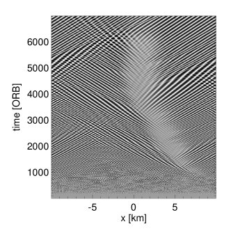
Figure 11: Stroboscopic space-time diagram (left panel) and final power spectrum of the surface mass density field (right panel) for the same non-isothermal integration as in Figure 10 with the $\tau_{20}$-parameters.

5.2 Hydrodynamical Integrations Including Radial Self-Gravity

5.2.1 Isothermal Model

In this section we describe our hydrodynamic model results with radial self-gravity, starting with the isothermal model. The initial state for all integrations is spectral white noise down to length scales $\lambda\sim 50\,\text{m}$. The computational regions for most integrations have radial dimension $L_{x}=5\,\text{km}$ with a grid resolution $h=2.5\,\text{m}$. We find that our isothermal integrations show three qualitatively distinct types of behavior with increasing strength of self-gravity, i.e. with increasing ground state surface mass density $\sigma_{0}$.

For $\sigma_{0}\lesssim 200\,\text{kg}\,\text{m}^{-2}$ and the $\tau_{15}$-parameters ($Q_{0}\gtrsim 4$), the influence of self-gravity is weak, and the system constantly generates modes corresponding to the largest linear growth rates. These waves experience nonlinear interactions, resulting in modes with longer wavelengths. The spectrum accordingly shows a concentration of power on wavelengths $\lambda\lesssim 100\,\text{m}$, and energy scattered over a wide range of larger wavelengths which exceed the wavelengths characterizing the final state of the non self-gravitating integrations by large amounts. It is unclear whether this wavelength growth would halt at some finite value. The numerical time step becomes very small in this state, resulting in an impracticably slow integration. Thus, we find that in the isothermal model the regime of small self-gravity forces is difficult to probe with our numerical method. In the next section we will see that this difficulty does not occur in the non-isothermal model.

When increasing the value of $\sigma_{0}$, such that $200\,\text{kg}\,\text{m}^{-2}\lesssim\sigma_{0}\lesssim 600\,\text{kg}\,\text{m}^{-2}$ ($4\gtrsim Q_{0}\gtrsim 1.5$ for $\tau=1.5$), the system behaves very differently. Initially, we observe a fast development of multiple source/sink structures. Moreover, the wavelengths of the interacting waves grow fast. However, this growth slows down and halts at a certain wavelength. We observe that upon gradually increasing $\sigma_{0}$, this prevalent wavelength reduces in a monotonic manner. Since the wavelength of a nonlinear saturated overstable wave is proportional to its amplitude (SS2003, LO2009), the kinetic energy density is also a good proxy for the dominant wavelength of the overstable waves. Figure 12 shows the development of the kinetic energy densities of integrations with intermediate and high values of $\sigma_{0}$, confirming that higher values of the surface mass density result in states with smaller overall kinetic energy density, indicating a smaller dominant wavelength. We find that the outcomes of these computations exclusively consist of (quasi-)stable source/sink states. Examples are presented in Figure 13. By comparing Figures 7 and 13 one can see that the sources and sinks in the integrations with self-gravity are more narrow than in the case of vanishing self-gravity, indicating a stronger interaction between the counter-propagating wave trains. The stable source and sink structures connect patches of counter-propagating traveling waves with spatially constant wavelength. Integrations for more than 20,000 orbits have been performed throughout which these configurations persisted, without any signs of numerical instability or merging of sinks and sources.

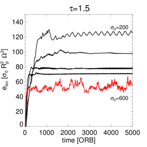
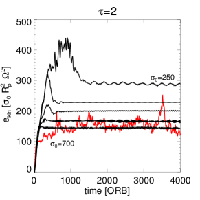
Figure 12: Kinetic energy densities of isothermal integrations with different values $\sigma_{0}$. Curves with higher saturation energy correspond to smaller values of $\sigma_{0}$. Left: $\tau_{15}$-parameters with $\sigma_{0}=200,250,300,400\,\text{and}\,600\,\text{kg}\,\text{m}^{-2}$. Right: $\tau_{20}$-parameters with $\sigma_{0}=250,300,350,400,500\,\text{and}\,700\,\text{kg}\,\text{m}^{-2}$. The red curves in both panels correspond to the highest value of $\sigma_{0}$, respectively.

Further increasing $\sigma_{0}$ leads to numerical instability of our scheme, unless we reduce the time steps by a large factor. We performed two integrations in this regime ($\tau=1.5$ with $\sigma_{0}=600\,\text{kg}\,\text{m}^{-2}$ and $\tau=2$ with $\sigma_{0}=700\,\text{kg}\,\text{m}^{-2}$) with time steps $f_{t}\sim 0.01$. In these we find source/sink structures which become chaotic such that these disappear and reappear continuously, showing a stochastic peculiar motion. The kinetic energy for these integrations (red curves in Figure 12) undergoes strong fluctuations, caused by fluctuations in the dominant wavelength.

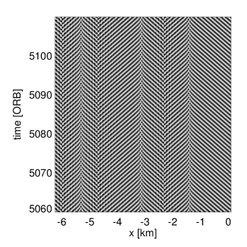
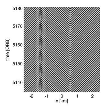
Figure 13: Snapshots of hydrodynamic quantities (upper panels) and orbit-resolved (sampling interval of $0.02\,\text{ORB}$) space-time diagrams (lower panels) of stable source/sink states resulting from isothermal self-gravitating integrations with the $\tau_{15}$-parameters. Left: $\sigma_{0}=250\,\text{kg}\,\text{m}^{-2}$ ($Q_{0}=3.2$, $\lambda\approx 170\,\text{m}$). Right: $\sigma_{0}=400\,\text{kg}\,\text{m}^{-2}$ ($Q_{0}=2.0$, $\lambda\approx 120\,\text{m}$).

Notable is that none of our self-gravitating isothermal integrations presented here produces final states consisting of a single traveling wave mode. We additionally performed integrations where the seed consisted of a single overstable mode with $50\,\text{m}\lesssim\lambda\lesssim 100\,\text{m}$. These integrations either develop source/sink structures, leading to the states described above, or they exhibit a unidirectional wave train with ever growing wavelength until the numerical time step becomes so small that the further evolution cannot be followed anymore.

5.2.2 Non-isothermal model

We now turn to the results of the non-isothermal integrations including the radial component of self-gravity. Here the calculation box for most integrations is $L_{x}=20\,\text{km}$ with $h=2.5\,\text{m}$. Integrations with high surface densities $\sigma_{0}\geq 700\,\text{kg}\,\text{m}^{-2}$ are conducted in smaller boxes ($L_{x}=5\,\text{km}$). For these we find it necessary to employ a finer grid ($h=1\,\text{m}$), as the hydrodynamic quantities exhibit very sharp transitions.

Figure 14 shows the evolution of the kinetic energy density of integrations with the $\tau_{15}$ and the $\tau_{20}$-parameters with different surface densities $\sigma_{0}$. The results show similarities to the isothermal results (12). For sufficiently large $\sigma_{0}$ the main effect of self-gravity is a reduction of the final state wavelengths, and thus the energy of ordered motions $e_{kin}$. For small self-gravity forces, the final state is dominated by modes with wavelengths larger than those found for the non self-gravitating case (Section 5.1.2). This result was also found within the isothermal model. Nevertheless, the non-isothermal system evolves into an ordered final state which is not polluted by modes with smaller wavelengths, as can be seen for example in Figure 15.

Similar to the non self-gravitating integrations (Section 5.1), the initial stage for all $\sigma_{0}$-values is chaotic, with strong spatio-temporal fluctuations of all hydrodynamic quantities. During this stage $e_{kin}$ is increasing more or less strongly with time. The intermediate source/sink phase, though, is different if a moderate radial self-gravity is included. The sources and sinks are more numerous and narrower than for the non self-gravitating case. The source/sink pattern resembles the one found for the isothermal model with intermediate values of $\sigma_{0}$ (cf. Figure 13), i.e. the structures appear more stable, showing less fluctuations. Quasi-stable source/sink states, persisting for more than 10,000 orbits, are found for small, intermediate and large values of $\sigma_{0}$. For instance the integration shown in Figure 15 represents such a case with small $\sigma_{0}=125\,\text{kg}\,\text{m}^{-2}$. Another example is the case $\sigma_{0}=600\,\text{kg}\,\text{m}^{-2}$ for $\tau=2$, where a source/sink pair reveals itself through small, persistent fluctuations in the (leveled) kinetic energy curve (Figure 14), as the waves connecting these structures undergo small fluctuations in phase and amplitude.

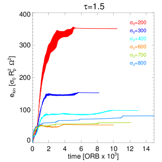
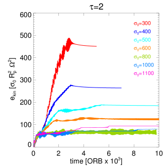
Figure 14: Evolution of the kinetic energy for non-isothermal hydrodynamic integrations with different $\sigma_{0}$-values. The final wave train energies show a monotonic decrease as a function of $\sigma_{0}$ which reverses around $\sigma_{0}=600\,\text{kg}\,\text{m}^{-2}$ for $\tau=1.5$ ($\sigma_{0}=700\,\text{kg}\,\text{m}^{-2}$ for $\tau=2$).

For larger $\sigma_{0}$ with the $\tau_{20}$-parameters the hydrodynamic field quantities become increasingly distorted during the initial and intermediate stages where the different wave patches exhibit in many cases standing wave-like amplitude fluctuations. This phase can persist for a long time, as for the case $\sigma_{0}=800\,\text{kg}\,\text{m}^{-2}$ with $\tau=2$ (right panel in Figure 14, see also Figure 16 in Section 5.3). This behavior and the fact that the overstable oscillation frequency for large $\sigma_{0}$ is in general significantly different from the orbital frequency makes it harder to identify source and sink structures in (stroboscopic) space-time plots. For integrations with $Q_{0}\lesssim 1$ with $\tau=1.5$ we find, after a short initial chaotic stage, an elongated stair-case process in which wavelength and kinetic energy undergo a slow stepwise increase. This is seen in the curves for $\sigma_{0}=700\,\text{kg}\,\text{m}^{-2}$ and $\sigma_{0}=800\,\text{kg}\,\text{m}^{-2}$ with $\tau=1.5$ (left panel in Figure 14), and also in the curve for the case $\sigma_{0}=1,100\,\text{kg}\,\text{m}^{-2}$ with $\tau=2$ (right panel in Figure 14), subsequent to a highly distorted standing wave phase. The final state traveling waves of these integrations possess small phase and amplitude perturbations.

Although not verified for all our integrations, it is likely that sink and source structures eventually merge and vanish, thus resulting in single mode traveling waves. This is a notable difference to the results of our isothermal integrations with radial self-gravity, where we did not find stable (on timescales of at least some 10,000 ORB) final states consisting of a single unidirectional traveling wave.

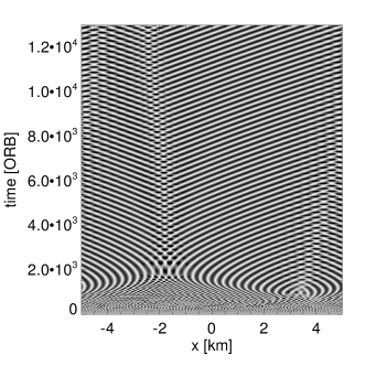
Figure 15: Non-isothermal integration with the $\tau_{15}$-parameters and $\sigma_{0}=125\,\text{kg}\,\text{m}^{-2}$. The right panel shows the final power spectrum. The space-time diagram (left panel) is stroboscopic, giving the impression of a reversal of the phase velocity of the waves (see also Figure 27). The system evolves into an ordered source/sink state with a prevalent wavelength exceeding that of the case $\sigma_{0}=0$. However, for larger $\sigma_{0}$ the wavelengths in gravitating integrations are shorter than those with $\sigma_{0}=0$.

Our isothermal and non-isothermal models utilize a significantly different equation of state, given by Equations (8) and (20), respectively. In Section 2 we have shown that, on a linear level, the effects of the temperature equation on overstable waves are mildly stabilizing (see Figure 1). For an assessment of thermal effects in the nonlinear regime we perform hydrodynamic integrations with the isothermal $\tau_{15}$ and $\tau_{20}$-parameters, but adopting the density dependence of pressure ($p_{s}$) of the non-isothermal model (Table 3), instead of $p_{s}=1$ for the ideal gas relation. In this case we find with both parameter sets a saturation of overstability similar to the one obtained in the non-isothermal system, but with considerably larger saturation wavelengths. Thus, the inclusion of temperature variations leads to a saturated state of the viscous overstability with considerably less kinetic energy contained in the nonlinear wave trains, which amounts to a smaller saturation wavelength.

5.3 N-Body Simulations

In the following we turn to the results of our N-body simulations (cf. Section 4.2) with varying magnitude of the radial self-gravity force. In all conducted simulations the waves undergo a chaotic initial stage with standing wave like patterns, similar to those encountered in hydrodynamic integrations with large surface densities $\sigma_{0}$. The duration of this stage is found to increase with increasing $\sigma_{0}$. Systems with small and intermediate $\sigma_{0}$ evolve into uniform traveling wave states within a few thousand orbits. Source and sink structures are not found in any of the runs. This absence might be explained by the relatively small size of the simulation box ($L_{x}\leq 5\,\text{km}$) used here, when compared to our hydrodynamic integrations (Figures 11 and 15) as well as the non-selfgravitating N-body simulation presented in Figure 6 in RL2013.

As an illustration (Figure 16) we plot snapshots of various quantities across the simulation box for two runs ($\sigma_{0}=0$ with $\tau=1.5$ and $\sigma_{0}=800\,\text{kg}\,\text{m}^{-2}$ with $\tau=2$) and compare with results from non-isothermal hydrodynamical integrations. Overall the hydrodynamic description is able to capture quite well most of the salient features of the wave trains, such as the dominant wavelength and the shapes of the velocity fields and the surface density. In the case $\sigma_{0}=800\,\text{kg}\,\text{m}^{-2}$ N-body and hydrodynamic systems both exhibit complicated standing wave like patterns. The most notable differences are in the profiles of the velocity dispersion. In the simulations the velocity dispersion does not attain values smaller than $R_{p}\Omega\sim 0.2\,\text{mm/s}$, due to nonlocal viscous heating. The hydrodynamic description does not capture this lower bound and, on the other hand, overestimates the temperature peaks in systems with large $\sigma_{0}$.

For the N-body simulations shown in Figure 16, and also for the computation of the kinetic energy (see below), a tabulation is performed of different quantities across the simulation box into $n$ radial zones of width $\Delta x=L_{x}/n$, covering the whole azimuthal and vertical extent of the simulation box. For the computation of velocity fields we tabulate the particle’s individual radial, vertical and azimuthal velocities relative to the Keplerian motion. The mean values of the radial and azimuthal velocities, taken over all particles in the zone at radial location $x$, are then identified with the hydrodynamic velocity fields $u(x)$ and $v(x)$, respectively [cf. Equation (14)]. These describe the collective particle motion in radial and azimuthal direction, respectively, which in our simulations is due to viscous overstability. The resulting vertical velocity field takes negligible values, since the collective vertical particle motion in (overstable) wave trains is anti-symmetric with respect to the plane $z=0$, so that contributions from particles above and below the plane cancel. This is clearly seen in the particle’s vertical coordinates $Z$ (Figure 16) and is a consequence of the near incompressibility of the simulated ring state. Furthermore, the standard deviations of the velocity components in a given zone define the diagonal components of the velocity dispersion tensor (Section 4.1), $\hat{C}_{xx}$, $\hat{C}_{yy}$ and $\hat{C}_{zz}$. These determine the velocity dispersion

$$c(x)=\left[\frac{1}{3}\left(\hat{C}_{xx}^{2}+\hat{C}_{yy}^{2}+\hat{C}_{zz}^{2}\right)\right]^{1/2},$$

which relates to the hydrodynamic temperature via $c=T^{1/2}$. The scaled surface density $\sigma(x)/\sigma_{0}$ is obtained by scaling the number of particles in the zone at radial location $x$ with the average number of particles per bin in the simulation box.

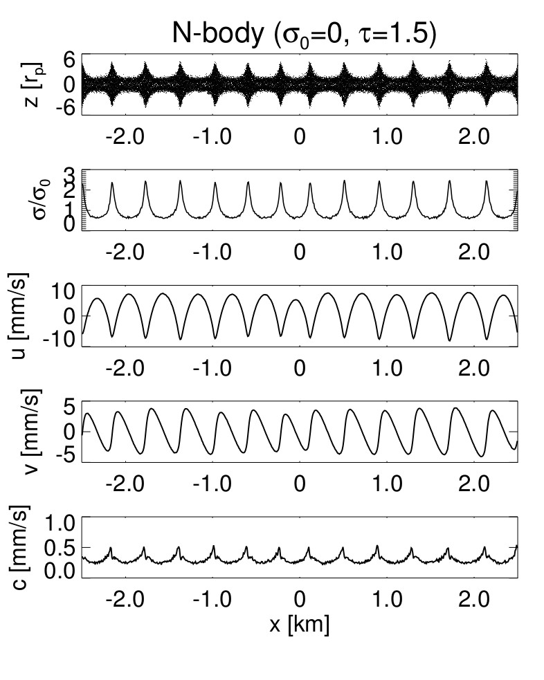
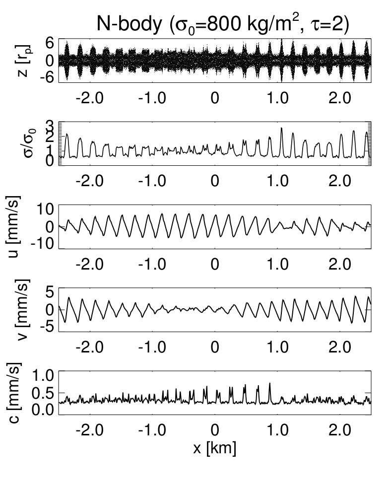
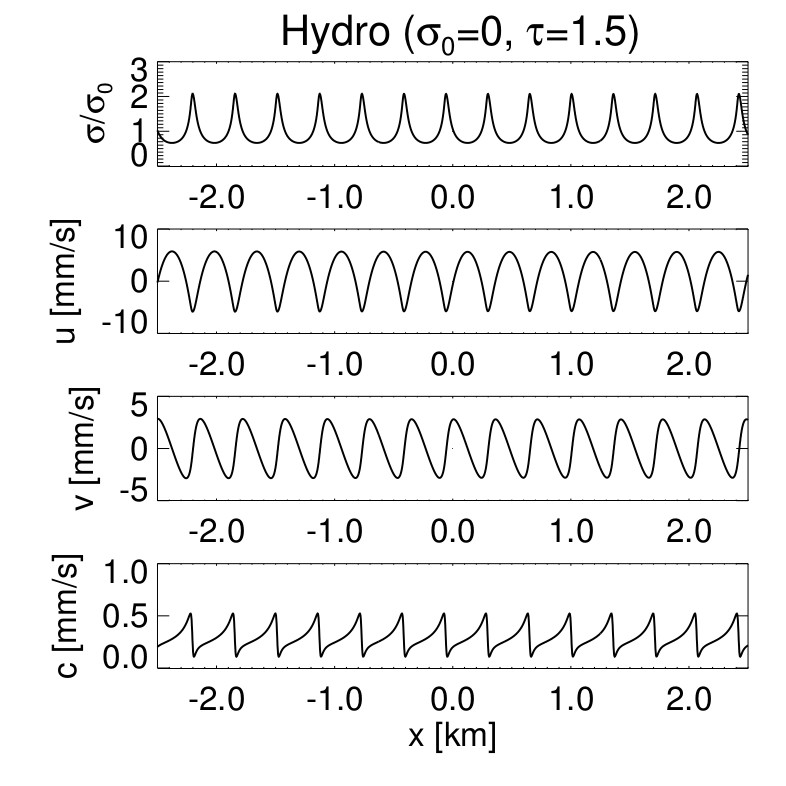
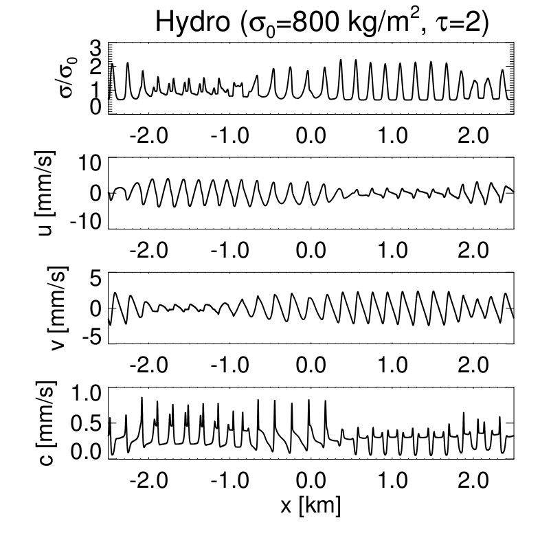
Figure 16: Comparison of saturated states of the viscous overstability in simulations (upper panels) and the non-isothermal hydrodynamic model (lower panels). The left column displays non-selfgravitating systems with $\tau=1.5$. The final states in both panels are left traveling waves. The right column shows systems with strong self-gravity. For this case both the N-body simulation and the hydrodynamic integration result in persistent standing wave patterns, exhibiting strong amplitude fluctuations. All displayed cases correspond to $\Omega_{z}=3.6$. For the hydrodynamic integration with $\sigma=0$ we used $L_{x}=10\,\text{km}$ with $h=2.5\,\text{m}$. For the case $\sigma_{0}=800\,\text{kg}\,\text{m}^{-2}$ we utilized $L_{x}=5\,\text{km}$ with a finer grid ($h=1\,\text{m}$), required to accurately capture the sharp spatial transitions of numerical quantities. The N-body simulations were conducted in boxes with $L_{x}=5\,\text{km}$.

Figure 17 displays the evolution of the mean kinetic energy (39) for simulations with $\Omega_{z}=3.6$ and with optical depths $\tau=1.5$ and $\tau=2$ for different values of $\sigma_{0}$. These simulations were conducted in boxes of radial size $L_{x}=5\,\text{km}$ (cf. Table 4.2). Similar to the results of the hydrodynamic computations we find that the kinetic energy $e_{kin}$ in the overstable oscillations drops with increasing $\sigma_{0}$. However, in contrast to hydrodynamics, this trend holds within a wider range of surface mass densities $\sigma_{0}$. Deviations from this monotonic behavior occur only for very small and very large values of $\sigma_{0}$. For very small nonzero $\sigma_{0}$ the spectral range of the developing nonlinear overstable modes is relatively wide. It extends to larger wavelengths than for the non-selfgravitating case, leading to an increased kinetic energy density. For high $\sigma_{0}$ the trend of a decreasing kinetic energy seems to level off. Similar to the hydrodynamic results (Figure 14) this occurs at about $\sigma_{0}=700\,\text{kg}\,\text{m}^{-2}$ for $\tau=1.5$ and at a slightly larger value for $\tau=2$.

We performed several tests to assure that the radial box size used for our N-Body simulations is sufficiently large (Figure 18). We find that the box size is not affecting the outcome of the simulations.

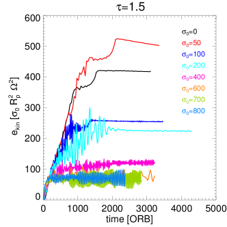
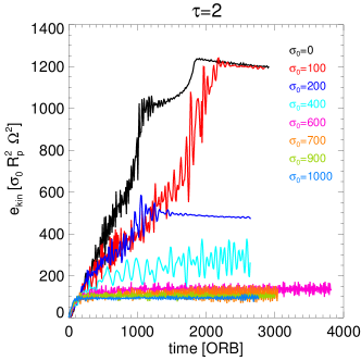
Figure 17: Evolution of the kinetic energy densities in simulations with optical depths $\tau=1.5$ and $\tau=2$ and $\Omega_{z}=3.6$ for different $\sigma_{0}$ (in $\text{kg}\,\text{m}^{-2}$) (see Table 4.2 for parameters). The behavior of $e_{kin}$ with changing $\sigma_{0}$ is qualitatively similar as in the non-isothermal hydrodynamic model (Figure 14), but the overstable waves are temporarily and spatially less uniform, leading to the large fluctuations in the kinetic energy curves.

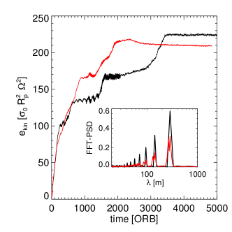
Figure 18: Simulations conducted to explore possible effects of the finite box size. Left: The curve for $t\leq 5,000\,\text{ORB}$ represents the kinetic energy density of a simulation with $\tau=1.5$, $\Omega_{z}=3.6$ and $\sigma_{0}=150\,\text{kg}\,\text{m}^{-2}$ in a box with $L_{x}=2\,\text{km}$. The final state of this simulation at $t=5,000\,\text{ORB}$ is taken as an initial state for three new simulations in larger boxes with $L_{x}=4\,\text{km}$. One of these simulations keeps the value of $\sigma_{0}=150\,\text{kg}\,\text{m}^{-2}$. The other two continue with $\sigma_{0}=0$ and $\sigma_{0}=600\,\text{kg}\,\text{m}^{-2}$, respectively. The curve for $\sigma_{0}=150\,\text{kg}\,\text{m}^{-2}$ for $t>5,000\,\text{ORB}$ shows that the box size is not affecting the overstability. On the other hand, the other two runs begin to evolve in a manner consistent with the newly imposed surface mass density. The arrows indicate the final values of $e_{kin}$ in the simulations with $\sigma_{0}=0$ and $\sigma_{0}=600\,\text{kg}\,\text{m}^{-2}$ displayed in Figure 17. Right: Comparison of two simulations with $\tau=1.5$, $\Omega_{z}=3.6$ and $\sigma_{0}=300\,\text{kg}\,\text{m}^{-2}$ but different box sizes $L_{x}=2\,\text{km}$ and $L_{x}=8\,\text{km}$, respectively. The insert plot represents the final power spectra of the radially tabulated particle surface number densities. The qualitative similarity of both runs underlines the consistency of results obtained with the two box sizes.

In Figure 19 we compare final values of the velocity dispersion, averaged over the simulation box and time, denoted by $\langle c\rangle$. Also shown are collision frequencies of simulations with different $\Omega_{z}$ and the same optical depth $\tau=1.5$, as a function of $\sigma_{0}$. Results of $\langle c\rangle$ from non-isothermal hydrodynamical computations, drawn for comparison, agree fairly well with the N-body simulation results. The collision frequencies $\omega_{c}$ of the simulated systems are generally high due to the enhanced vertical frequency $\Omega_{z}$, and the growth of overstable modes even leads to further enhancement of up to some $20\%$. From the curves one may deduce that it is not the amount of energy ($e_{kin}$) contained in overstable oscillations but the magnitude of the radial self-gravity force which dictates the collision frequency. This is evidenced by the fact that in contrast to $e_{kin}$, the values of $\omega_{c}$ increase with increasing $\sigma_{0}$. This increase of the collision frequency in the nonlinear wave trains is not accounted for in the hydrodynamic model. Therefore, particularly for strong radial self-gravity it can be expected that in the nonlinear state of viscous overstability the hydrodynamic model underestimates collisional transport effects, in particular the nonlocal pressure modeled through Equation (8).

Simulations with $\Omega_{z}=2$ exhibit significantly smaller collision frequencies than those with $\Omega_{z}=3.6$. This results in a smaller collisional momentum flux and thus a smaller value of the viscous parameter $\beta$ (cf. Section 2). The overstable wave trains found in systems with $\Omega_{z}=2$ have generally smaller amplitudes than those in systems with $\Omega_{z}=3.6$ and are less capable of heating up the system [Figure 19 (left panel)].

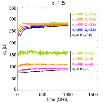
Figure 19: Left: The velocity dispersion of saturated overstable wave trains, averaged over the simulation box and a time interval of at least 100 orbits, as a function of the ground state surface density $\sigma_{0}$ for simulations with optical depth $\tau=1.5$ and different vertical frequencies $\Omega_{z}$. The simulations with $\Omega_{z}=3.6$ (asterisks) are the same as in Figure 17 (left panel), conducted in boxes with $L_{x}=5\,\text{km}$ and with a coefficient of restitution $\epsilon=0.5$. For the simulations with $\Omega_{z}=2$ (plus symbols) we utilized $L_{x}=2\,\text{km}$ and $\epsilon=\epsilon_{b}$ [Equation (48)]. Also plotted are results from corresponding hydrodynamic computations. The hydrodynamic results for $\Omega_{z}=3.6$ (squares) are the same as in Figure 14 (left panel). The hydrodynamic results corresponding to $\Omega_{z}=2$ (triangles) are conducted with $L_{x}=10\,\text{km}$. The horizontal dashed lines indicate the ground state temperatures of the two parameter sets with $\tau=1.5$ (Table 3). Right: Evolution of the collision frequencies of the same simulations.

6 Saturation Wavelength of Viscous Overstability

One important observable quantity is the wavelength of overstable oscillations in Saturn’s rings, that establishes as the result of the long-term nonlinear evolution of the wave pattern. From the hydrodynamic models and the N-body simulations we define the final, saturated wavelength $\lambda_{p}$ (the subscript $p$ denoting prevalent), as the wavelength with the largest Fourier amplitude in the saturated surface mass density field. Figure 20 summarizes our results. Generally, $\lambda_{p}$ decreases with increasing surface mass density of the ring, until, for large $\sigma_{0}$, it settles on values that lie around $100-200\,\text{m}$, depending on the precise optical depth and the vertical frequency enhancement. At small surface densities $\sigma_{0}<200-300\,\text{kg}\,\text{m}^{-2}$ the saturated wavelengths from the N-body simulations deviate from the hydrodynamic ones, in that they connect smoothly to the wavelength that establishes in non-selfgravitating simulations. In the hydrodynamic models, in contrast, the saturated wavelengths rise to considerably larger values for small surface mass density, exceeding by far the wavelength of non-selfgravitating systems. We will return to a discussion of these deviations at small $\sigma_{0}$, as well as the behavior at large $\sigma_{0}$ in Sections 6.1, 6.2.

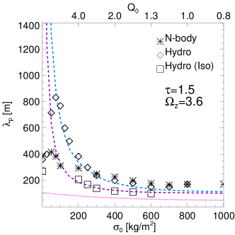
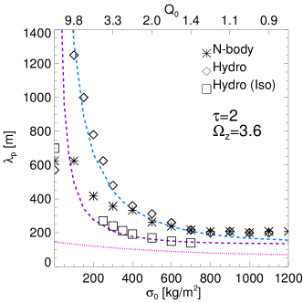
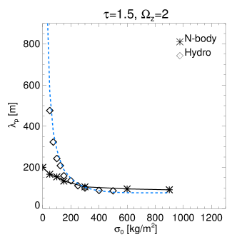
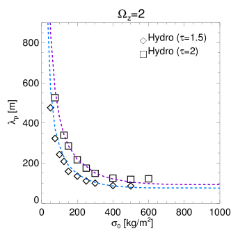
Figure 20: Saturated, prevalent overstable wavelengths from N-body simulations and hydrodynamic non-isothermal (“Hydro”) and isothermal (“Iso”) models. In all frames the dashed curves are the empirical relation (55) with $C=1.4$. For comparison the dotted curves in the upper frames represent the wavelengths of highest linear (non-isothermal) growth rates, following from Equation (16). The isothermal results in the upper frames correspond to the limit $G_{T}\to\infty$ with $p_{s}=1$ (Section 2).

For a wide range of intermediate surface mass densities the hydrodynamic prevalent wavelengths follow the simple empirical relation (dashed lines in Figure 20)

$$\lambda_{p}=C\lambda_{zero}(\sigma_{0}).$$ (55)

Here, $\lambda_{zero}(\sigma_{0})$ is the wavelength of vanishing linear group velocity (Figure 2), which in turn corresponds to the slowest linear oscillation frequency [cf. Equation (22)]. We find that one single factor $C=1.4$ fits quite well all results for different optical depths and different enhancements of the vertical frequency. Non-isothermal and isothermal models both follow this trend with the same factor $C$, if one takes into account the difference in $\lambda_{zero}$ for the two cases. Also, the saturation wavelengths from the N-body simulations, in the range of surface mass densities $\sigma_{0}\gtrsim 300\,\text{kg}\,\text{m}^{-2}$, settle to attain values that are very similar to the non-isothermal hydrodynamic ones.

6.1 Nonlinear Dispersion Relation

The empirical relation (55) between the nonlinearly saturated wavelengths and the wavelength of vanishing group velocity from the linear dispersion relations encourages us to determine the nonlinear dispersion relation of overstable oscillations and compare its curve to the saturated $\lambda_{p}$. To this end we extract from the hydrodynamic models the nonlinear frequency for a given wavelength $\lambda$ from integrations with a calculation region of size $L_{x}=\lambda$. To mimick radial self-gravity contributions from distant wave parts, we use an extended force kernel in the self-gravity calculation (Section 4.1.2). In contrast to the measurements of the linear frequencies (Section 4.1.3) now a large amplitude single wavelength mode is seeded so that only this mode saturates. Its evolution can be followed for at least 50 orbital periods, until, in cases where $\lambda$ is very large, modes with shorter wavelengths take over before the amplitude of the seeded mode is fully saturated. The frequency is then determined with a Lomb normalized periodogram, as for the linear frequencies. The nonlinear dispersion relation from N-body simulations is determined in a similar manner using a calculation box with $L_{x}=\lambda$ and applying a large amplitude sinusoidal initial seed for the $m=1$ oscillation mode (radial velocity amplitudes of the order of $10R_{p}\,\Omega$). The radial self-gravity (54) is calculated from all modes down to about $10\,\text{m}$, to assure that the nonlinear shape of the oscillating wave crests is resolved. As for the hydrodynamical model, the initial period during which the prominent mode adjusts its oscillation toward the final nonlinearly saturated state is excluded.

The hydrodynamic nonlinear dispersion relations obtained in this manner are shown in Figure 21 for the $\tau_{15}$ and the $\tau_{20}$-parameters (upper frames) and additionally for a smaller vertical frequency $\Omega_{z}=2$ and an isothermal system (lower frames). Generally, we find that for self-gravitating systems the wavelength of minimal frequency is shifted by nonlinearity to larger values. For the non-isothermal model (panels a-c) also the minimal frequency itself is larger, compared to the linear dispersion relation (dashed curves). For non-selfgravitating systems such a nonlinear shift, attributed to the action of pressure, was already noted by LO2009 (see their Equations (33) and (34) as well as their Figure 4). Also thermal effects alter the nonlinear frequencies, mitigating the pressure-related increase. At larger $\lambda$ the curves for the linear and nonlinear dispersion relations cross. At these large wavelengths self-gravity begins to dominate the deviation of the oscillation frequency from the Keplerian value.

The nonlinear frequency reduction due to self-gravity is analogous to the nonlinear wavenumber reduction found for resonant spiral density waves in a dense ring, for which pressure forces play a minor role (Shu et al., (1985); Lehmann et al., (2016)). In the isothermal model (panel d), with the ideal gas equation of state, the presence of any substantial self-gravity force results in a nonlinear reduction of the oscillation frequencies.

One notes that all nonlinear frequency curves converge to the linear curves at small $\lambda$, since the saturation amplitudes of the wave trains scale linearly with $\lambda$ (SS2003, LO2009) and nonlinear effects eventually vanish as the wavelengths approach the linear stability boundary. For sufficiently long wavelengths the effects of pressure and self-gravity vanish and the nonlinear curves also approach the linear limit.

We find that the prevalent wavelengths in the large-scale, self-gravitating hydrodynamic models (asterisk symbols in Figure 21) depend in a systematic manner on the minimum of the corresponding nonlinear frequency curve. This suggests that nonlinearity accounts for much of the deviation from unity of the factor $C$ in the empirical relation (55). For instance, the saturation wavelengths of integrations with the $\tau_{15}$-parameters and $\sigma_{0}\leq 600\,\text{kg}\,\text{m}^{-2}$ (excluding the case $\sigma_{0}=0$) are very close to the minimum of the nonlinear dispersion relation [panel (a) in Figure 21]. This implies very small group velocities [Equation (23)] of the saturated wave trains (see Figure 30 in Appendix C). However, with increasing $\sigma_{0}$ the values of $\lambda_{p}$ gradually depart from the minimum toward larger wavelengths for all displayed cases in Figure 21. This apparent inconsistency will be resolved in Section 6.2.

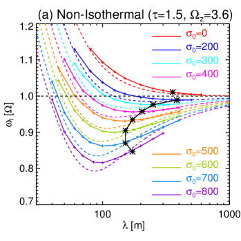
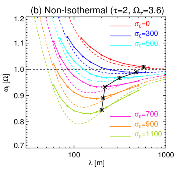
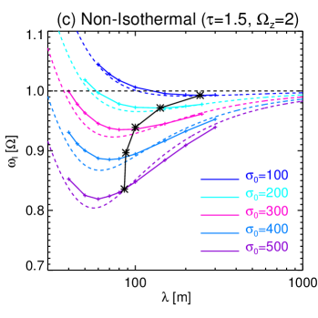
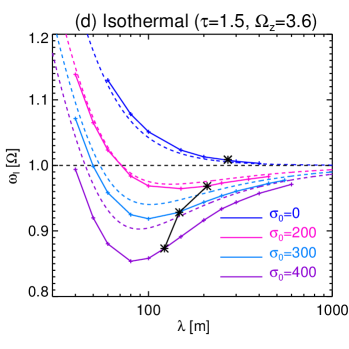
Figure 21: Nonlinear hydrodynamic oscillation frequencies extracted from computations of saturated traveling waves of different wavelengths and for different parameter sets in periodic domains with radial size corresponding to one wavelength. The solid curves represent different surface densities $\sigma_{0}$. The dashed curves are the linear oscillation frequencies from numerical solution of Equation (16). The over-plotted asterisks represent the final states of large-scale runs from Figure 20.

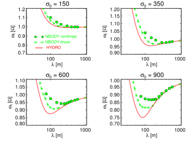
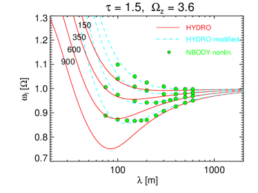
Figure 22: Oscillation frequencies in N-body simulations performed with four different surface densities ($\sigma_{0}=150,\ 350,\ 600,\ 900\,\text{kg}\,\text{m}^{-2}$). All simulations used $\tau=1.5$, $\Omega_{z}=3.6$, and relation (48) for $\epsilon(v)$. Left: predictions of the linear, non-isothermal hydrodynamical model are indicated with solid red curves, while the symbols stand for N-body simulations, with frequencies measured both during the linear growth period (open boxes), and from the final nonlinear saturated state (filled circles). Right: the nonlinear oscillation frequencies measured from N-body simulations performed with different surface densities are compared to the linear hydrodynamical prediction (red solid lines), as well as a modified hydrodynamical model (blue dashed lines), which corresponds to a 2-fold value of the pressure coefficient $p_{s}$, keeping all other quantities unchanged.

In the N-body simulations the nonlinear dispersion relation assumes generally larger frequencies than the linear one (Figure 22, left panel). The latter, determined from simulations with small-amplitude overstable waves, has in turn larger frequencies than the linear dispersion relation predicted by the hydrodynamic model. Moreover, for the N-body simulations the minimum of the nonlinear oscillation frequency is shifted towards larger wavelengths, as is the case for the hydrodynamic nonlinear dispersion relation (cf. Figure 21). Much of the difference between the hydrodynamic model and the N-body simulations can be attributed to the altered action of pressure in the nonlinearly saturated state. That is, if we modify the pressure coefficient $p_{s}$ of the hydrodynamic model by a factor of two, the hydrodynamic linear dispersion relation matches very well the nonlinear dispersion relation from N-body simulations for a wide range of surface mass densities (Figure 22, right panel). Recall that a modification of $p_{s}$ by a factor of 1.4 led to a similarly good agreement between the linear frequencies and growth rates (see Section 4.2.2 and Appendix B.2).

Also the prevalent wavelengths from large-scale N-body simulations ($L_{x}\geq 2\text{km}$) lie close to the minimum of the nonlinear oscillation frequency in the self-gravitating systems (Figure 23), reminiscent of the empirical relation (55). The group velocity of the waves vanishes at this frequency minimum and therefore any spacial variations in the wave pattern will not propagate anymore. For this reason the interaction of spatially separated wave states, with slightly different properties, will become weaker, and ultimately vanish, when the wavelength approaches the value of zero group velocity. We expect that in the limit $t\rightarrow\infty$ the simulations evolve towards this wavelength.

On the timescales accessible to the numerical exploration (thousands to ten thousands of orbits) we expect a belt of quasi-stable wavelengths around this minimum, which practically do not evolve. To explore this possibility (see also Appendix B.3) we perform simulations where a non-sinusoidal large-$\lambda$ seed is employed, with a wavelength very close to the frequency minimum of the nonlinear dispersion relation. In practice the initial positions and velocities of the simulation particles for this seeded state are taken from the final state of a simulation with smaller surface mass density and a larger saturated $\lambda$ (the starting points of the arrows in Figure 23). The diamond symbols mark the alternative final states reached in these new simulations (end points of the arrows). In this way arrows in the figure indicate the evolution of the prevalent wavelengths in the new, large-scale simulations. For $\sigma_{0}=600\,\text{kg}\,\text{m}^{-2}$ we find that two simulations with different size ($L_{x}=2$ and $4\,\text{km}$) reach slightly different final states with $\lambda_{p}=250\,\text{m}$ and $\lambda_{p}=210\,\text{m}$, respectively, both being very close to the minimum of the overstable oscillation frequency.

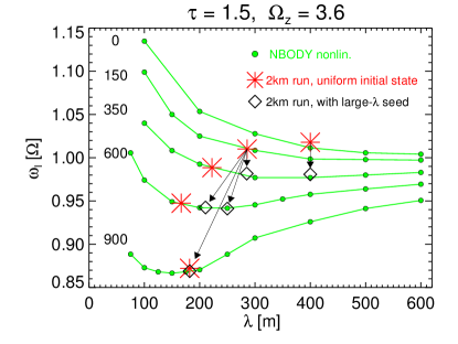
Figure 23: Nonlinear oscillation frequencies as a function of wavelength from N-body simulations (solid curves with circles). Large asterisk symbols mark the wavelength and frequency of the saturated state at the end of simulations ($t\sim 5,000\,\text{ORB}$) with $L_{x}=2\,\text{km}$ where overstability evolved from an initially uniform state. Although there are no obvious signs of further wavelength growth, it cannot be excluded that this might happen on much longer timescales. The diamond symbols indicate alternative final saturated states, which are stable on the timescales accessible to the simulations. These have evolved from different initial states as indicated by the arrows (see text).

In the limit of vanishing surface mass density the wavelength of the minimum oscillation frequency tends to very large values, theoretically approaching infinity. But especially for small surface mass density the minimum becomes very shallow. The particle flow in N-body simulations is subject to a variety of fluctuations (small non-axisymmetries, low contrast particle clumping, variations in the scale height). Consequently, there exists a certain threshold surface mass density below which the system does not feel the effect of the minimum anymore. We believe that this is the reason for the deviation in the saturation wavelength of the N-body simulations and the hydrodynamic systems for small surface densities (Figure 20). In the idealized hydrodynamic models the wavelength follows even in the small $\sigma_{0}$ limit the curve implied by relation (55), formally diverging for vanishing surface mass density, with a non-smooth transition to the finite saturated wavelength of the non-selfgravitating case. The prevalent wavelengths of the N-body simulations, in contrast, converge monotonically to the non-selfgravitating value. The deviations of the hydrodynamic models from relation (55) at very small (but non-zero) surface mass densities we attribute to the influence of the finite size of the computational domain ($L_{x}$), which becomes important for these very large wavelengths (see Appendix B.1). The integration with $\sigma_{0}=0$ in Appendix B.1 demonstrates that in the non-selfgravitating case stable uniform traveling wave solutions exist for all wavelengths larger than some critical value, as has been shown by LO2009 for the isothermal limit.

We note that for small surface densities $\sigma_{0}\lesssim 150\,\text{kg}\,\text{m}^{-2}$ the applied frequencies of vertical motions $\Omega_{z}=2-3.6$ imply unrealistic disk scale heights smaller than one particle radius [cf. (51)]. When using a self-consistent self-gravity implementation, systems with such small surface densities would not be viscously overstable. Furthermore, for sufficiently large $\sigma_{0}$ ($Q_{0}$ well below unity), the N-body simulations exhibit a gravitational instability, while the hydrodynamical scheme runs into numerical instability.

6.2 Hydrodynamical Integrations with a Buffer-Zone

In Section 6.1 we found that the prevalent wavelength $\lambda_{p}$ of large-scale hydrodynamic integrations and N-body simulations closely follows the wavelength corresponding to the frequency minimum of the nonlinear dispersion relation of overstable waves. However, with increasing surface mass density $\sigma_{0}$ the hydrodynamic values of $\lambda_{p}$ are increasingly displaced from the minimum towards larger wavelengths (asterisk symbols in Figure 21).

Here we check for a possible artificial influence of the periodic boundary conditions on the nonlinear saturation mechanism and the resulting wavelength $\lambda_{p}$. Therefore we perform hydrodynamic integrations, starting from spectral white noise with the $\tau_{15}$-parameters and various surface densities $200\,\text{kg}\,\text{m}^{-2}\leq\sigma_{0}\leq 800\,\text{kg}\,\text{m}^{-2}$, where we include a buffer-zone in the computational domain ($L_{x}=6-8\,\text{km}$). For an example of such an integration see Figure 29 in Appendix B.3. As outlined before (Section 5.1.1), the buffer-zone prevents the system from settling on a uniform nonlinear wave train and should eliminate possible spurious effects on the long term evolution, provoked by the periodic boundary conditions (Latter and Ogilvie, (2010)). The saturation wavelengths we find for these integrations are for all values of $\sigma_{0}$ close to the nonlinear frequency minimum (Figure 24), in a more consistent manner than the values found in homogeneous periodic integration domains. In conclusion, the presence of a buffer-zone shifts the saturation wavelength closer to the frequency minimum of the nonlinear dispersion relation.

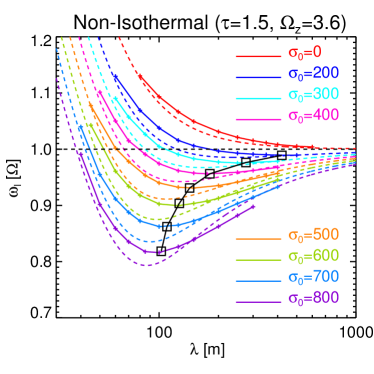
Figure 24: The same as figure 21a with the difference that now the symbols (open squares) mark the saturation wavelengths obtained from hydrodynamic integrations which started from low amplitude white noise and contained a buffer-zone in the calculation region (see also Figure 25).

In Figure 25 we display for the same integrations different ratios of $\lambda_{zero}^{lin}$ (the wavelength of the linear frequency minimum), $\lambda_{zero}^{nl}$ (the wavelength of the nonlinear frequency minimum) and $\lambda_{p}$ (the prevalent wavelengths of the final saturated states). Also these plots show that, albeit with some scatter, the saturation wavelength $\lambda_{p}$ tends to follow the nonlinear frequency minimum rather than the linear one.

It should be noted that it is difficult to obtain very accurate values of the involved nonlinear wavelengths for different reasons. On the one hand, the minima of the nonlinear frequency curves, which we can only probe with integrations as described in Section 6.1, are very mild for surface densities $\sigma_{0}\leq 400\,\text{kg}\,\text{m}^{-2}$. On the other hand, as already outlined in the discussion of Figure 23, the timescale of nonlinear evolution is prolonged if $\lambda_{p}$ is close to the nonlinear frequency minimum, requiring very long integrations.

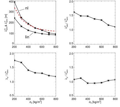
Figure 25: Plots involving the hydrodynamic ($\tau_{15}$-parameters) wavelengths corresponding to the linear frequency minimum ($\lambda_{zero}^{lin}$), the nonlinear frequency minimum ($\lambda_{zero}^{nl}$) and the saturation of overstability ($\lambda_{p}$), the latter being extracted from large-scale integrations which include a buffer-zone. In the upper left panel the labels “nl” and “lin” denote the curves of $\lambda_{zero}^{nl}$ and $\lambda_{zero}^{lin}$, respectively. The red dashed line is relation (55). Due to the buffer-zone, the prevalent wavelength in the final state can in some cases fluctuate within a given narrow range (about $5\%$). Here, and also in Figure 24 we display the smallest value of $\lambda_{p}$ for each surface mass density.

Most integrations presented in Figure 25 (and Figure 24) develop a persistent source/sink pair as a consequence of the buffer-zone, where the latter serves as the sink. In the cases with small surface densities ($\sigma_{0}=200-300\,\text{kg}\,\text{m}^{-2}$) all source and sink structures outside of the buffer-zone annihilate within a few thousand orbits so that the buffer-zone contains the remaining source/sink pair. In the case of very large surface density ($\sigma_{0}=800\,\text{kg}\,\text{m}^{-2}$) the pattern is more complicated and disturbed and it is not possible to identify source and sink structures. Nevertheless, in all integrations of Figure 25 the presence of the buffer-zone leads to the formation of nonlinear modes with wavelengths in direct vicinity of the nonlinear frequency minimum (cf. Appendix B.3).

As already outlined in Section 1, in Saturn’s rings one expects large-scale variations in the background parameters so that patches of overstable modes are permanently subject to perturbations. This situation might prevent the development of large uniform wave trains. The inclusion of a buffer-zone that damps overstability is a possible way to model this situation and should therefore provide a more realistic description than a (periodic) homogeneous integration region.

6.3 Variation of the Particle Radius

All simulations and integrations discussed thus far assume a mono-disperse ring consisting of particles with radius $R_{p}=1\text{m}$. A particle radius on the order of $1\text{m}$ follows from the formula for the geometric optical depth of a system of uni-sized spheres $\tau=\pi R_{p}^{2}\,\sigma/m_{p}$ (particle mass $m_{p}$) if one uses plausible parameters for Saturn’s A-ring [$\tau\sim 0.5-0.8$ (Colwell et al., (2009)), $\rho_{p}\sim 450\,\text{kg}\,\text{m}^{-3}$ (French et al., (2007)), $\sigma\sim 300\,\text{kg}\,\text{m}^{-2}$ (Tiscareno et al., (2007))].

A thorough investigation of the effects of a wider size distribution on viscous overstability in terms of N-body simulations is computationally not feasible at present, due to the very high particle collision rates. It can, however be expected that the presence of a particle size distribution has a mitigating effect on overstability (see Figure 5 in Salo, (2001)). Instead, we perform simulations with varying particle size, but keeping all other quantities (optical depth, elasticity law, surface mass density) unchanged. Note that this restriction can imply very unrealistic particle internal densities.

The effect of changing the particle radius on the saturation wavelength of overstability can be estimated as follows. For a large range of Toomre-parameters $Q_{0}>1$ relation (55) follows the estimate

$$\lambda_{p}\approx 2C\left(p_{s}-F_{2}\right)\lambda_{J}$$ (56)

with the Jeans-wavelength

$$\lambda_{J}=\frac{c_{0}^{2}}{G\sigma_{0}}.$$ (57)

This approximation follows directly from Equation (22) for $Q_{0}\gg 1$. In a dense ring the effective velocity dispersion [Equation (12)] scales roughly linearly with the particle radius, $c_{0}\sim R_{p}\Omega$, on account of the dominance of nonlocal pressure. Thus, we expect a roughly quadratic dependence of the saturation wavelength on the particle radius, $\lambda_{p}\sim R_{p}^{2}$, at least for a range of values $R_{p}$. For sufficiently small $R_{p}$, nonlocal effects would eventually diminish so that the condition for viscous overstability is not fulfilled anymore. Furthermore, for large values of the surface density $\sigma_{0}$ the system develops a gravitational instability for particle radii in the range $0.1-1\,\text{m}$.

Figure 26 shows the results of N-Body simulations performed with varying particle radius in the range $1-4\,\text{m}$ with a surface density $\sigma_{0}=900\,\text{kg}\,\text{m}^{-2}$ and the Bridges-type elasticity law (48). The radial width of the simulation region for these runs is chosen to depend quadratically on the particle radius, i.e. $L_{x}=2\,\text{km}\times(R_{p}/1\text{m})^{2}$ to accommodate for the expected behavior of the saturation wavelengths in these runs. The asterisk symbols in Figure 26 represent the resulting saturation wavelengths found for runs with periodic boundary conditions (as applied in all other N-Body simulations presented so far). The diamond symbols represent two runs where we adopt “spreading boundary” conditions. In these runs the initial particle positions do not fill out the complete radial extent of the simulation region. These simulations resemble the hydrodynamic integrations with a buffer-zone, since the nonlinear wave trains are damped out as they enter the rarefied region. This also implies the emergence of a sink structure since the boundaries represent a buffer region and are found to act as source. Eventually, viscous spreading causes the particles to fill the entire simulation box and the system becomes similar to our standard periodic boundary case. When this happens the system is able to sustain the larger prevalent wavelength attained during the expanding phase. The saturation wavelengths found in these runs are larger, and closer to the corresponding nonlinear frequency minima. Thus, in agreement with the hydrodynamic integrations presented in Section 6.2 as well as Appendix B.3, the presence of a buffer-zone shifts the prevalent wavelength of the saturated pattern closer to the nonlinear frequency minimum.

Figure 26: Saturation wavelengths of viscous overstability in N-Body simulations with varying particle radius and fixed optical depth $\tau=1.5$, vertical frequency $\Omega_{z}=3.6$ and surface density $\sigma_{0}=900\,\text{kg}\,\text{m}^{-2}$. The asterisks represent results from simulations with periodic boundaries (’PB’) while the diamonds correspond to simulations with spreading boundaries (’SB’). (See text).

Furthermore, in the absence of radial self-gravity ($\sigma_{0}=0$) we find a nearly linear dependence $\lambda_{p}\sim R_{p}$, which is expected as in this case the particle radius is the only physical scale parameter of the system.

6.4 Comparison to Previous Studies

Our results indicate that with increasing optical depth $\tau$, as well as with increasing vertical frequency enhancement $\Omega_{z}$ the saturation wavelength of the viscous overstabiliy increases. This is in agreement with LO2009 and LO2010, who have shown (in the absence of radial self-gravity) that the wavelength $\lambda_{st}$ of nonlinear traveling waves, which are the preferred saturation of the viscous overstability (SS2003), is a steeply increasing function of the viscous parameter $\beta$ (see their Table 3). This parameter in turn is an increasing function of the ground state optical depth $\tau$ (Salo et al., (2001)). A positive correlation between the overstable saturation wavelength of final state traveling waves and the equilibrium optical depth was later found in non-gravitating N-body simulations (RL2013). In N-body simulations, an increase of the parameters $\tau$ and $\Omega_{z}$ results in both cases in an increased collision frequency $\omega_{c}$. The latter is the quantitity which eventually affects the value of $\beta$. Nevertheless, a linear stability analysis of nonlinear wave train solutions of the system (1), including radial self-gravity, should be performed to verify our hydrodynamic results. A method similar to that used in LO2009 for the isothermal limit without radial self-gravity, might be suitable in the present case as well.

The results of Schmit and Tscharnuter, (1999) agree with ours in that their single isothermal integration with radial self-gravity resulted in a saturation of overstability with prevalent wavelengths of a few times the corresponding Jeans-wavelength. Indeed, the wavelength of vanishing linear group velocity, $\lambda_{zero}$, appearing in our relation (55) for the saturation wavelength, reads in the isothermal limit $\lambda_{zero}\approx 2p_{s}\lambda_{J}$ with the Jeans-wavelength (57).

7 Conclusion

We investigate the influence of self-gravity on the long term and large-scale evolution of axisymmetric waves induced by viscous overstability in a dense planetary ring. In our approach we use hydrodynamic models and N-body simulations. These take into account the effect of collective radial self-gravity, exerted by the wave pattern on the ring matter. Aspects of the vertical component of self-gravity are incorporated in terms of the overall enhancement of the vertical frequency of oscillations. The effect of direct particle-particle gravity is not included.

We find a reasonably good agreement between N-body simulations and the hydrodynamic treatment for the nonlinear saturation of the viscous overstability in a dense ring. For the majority of surface mass densities the main effect of the radial self-gravity force is a reduction of the saturation wavelength of viscous overstability. In particular, the agreement of both modeling approaches is good for surface densities $\sigma_{0}\gtrsim 300\,\text{kg}\,\text{m}^{-2}$, which are relevant for Saturn’s dense rings (Tiscareno et al., (2007); Hedman and Nicholson, (2016)), where overstability has been detected by Cassini instruments (Colwell et al.,, 2007; Thomson et al.,, 2007; Sremcevic et al.,, 2009; Hedman et al.,, 2014). The range of observed wavelengths $\lambda\sim 150\,\text{m}-250\,\text{m}$ compares well with the prevalent wavelengths we find in our models. Our results show that this length scale of saturation is closely related to the wavelength of minimal oscillation frequency of the nonlinear dispersion relation of oscillatory ring modes. This minimum exists only for a non-vanishing radial self-gravity force and it shifts to shorter wavelengths with increasing strength of radial self-gravity. Precisely at this minimum the group velocity of waves vanishes, so that the characteristic timescale for the nonlinear mode interaction diverges. Apparent deviations of the saturation wavelength from the nonlinear frequency minimum which we encounter in our results can have several reasons. Most importantly, we find that influences resulting from the application of periodic boundary conditions in a homogeneous model ring generally lead to an increase of the saturation wavelength in hydrodynamic integrations. But also the timescale of nonlinear evolution can prevent a proper determination of the saturation wavelength, particularly in N-body simulations. Moreover, the details of the numerical scheme to solve the hydrodynamic equations can have small but notable effects.

In our hydrodynamical integrations and N-body simulations with vanishing radial self-gravity we find, in agreement with previous studies (SS2003, LO2009, LO2010, RL2013), that viscous overstability saturates in form of nonlinear traveling waves. The same holds true if the radial self-gravity force is sufficiently weak. The nonlinear evolution toward this saturated state generally comprises source and sink structures at some point, separating counter-propagating wave trains. With increasing strength of self-gravity, saturated wave trains generally become more distorted, eventually showing persistent complex, standing-wave like interactions.

Generally, our hydrodynamic description that includes the energy equation yields a better match with N-body simulations than the isothermal approximation. We find that a good representation for the equation of state is essential to obtain an adequate description of the nonlinear saturation behavior of viscous overstability. In this vein, one route of future investigation could be the use of more suitable constitutive relations for dense particulate systems from the theory of granular matter (e.g. Haff, (1983); Hwang and Hutter, (1995)) in place of the power-law parameterizations (8)-(11) employed in this study. However, this will require also a self-consistent modeling of the disk’s vertical thickness (Borderies et al., (1985)). Another direction for future research could be an extension of the kinetic treatment by Latter and Ogilvie, (2008), so that it can be applied to dense systems, employing an Enskog collision term (Chapman and Cowling, (1970); Araki and Tremaine, (1986)). The considerable mathematical complexity of this approach could potentially be overcome by use of suitable approximations to solve the collision integrals (Hämeen-Anttila and Salo, (1993)). Such a treatment would allow to model the effect of additional modes in the components of the pressure tensor (Latter and Ogilvie,, 2008), which are not contained in the Newtonian approximation used in our study.

A major challenge will be the inclusion of direct particle-particle self-gravity and its effect on the large-scale, long-term evolution of viscous overstability in Saturn’s rings. In principle this can be achieved in terms of N-body simulations. But an investigation of the long radial scales we have studied in this paper is at present not feasible with this method, because of the prohibitively high CPU demand. It is known that the self-gravity of ring particles leads in large parts of Saturn’s rings to the formation of gravitational wakes (Salo,, 1992; Daisaka et al.,, 2001; Hedman et al.,, 2007; Colwell et al.,, 2007; French et al.,, 2007), non-axisymmetric structures of wavelengths below $100\,\text{m}$. N-body simulations with full self-gravity show that these wakes interact with overstable modes in a complex manner (Salo et al.,, 2001, 2018). We believe that the overall saturation behavior of viscous overstability, like the prevalent wavelength of overstable modes, and the occurrence of source/sink patterns, is captured by the axisymmetric gravity model we have employed in this paper. But gravitational wakes will have additional effects. For instance, the heating induced by the wakes, as well as their typical non-axisymmetric pattern superimposed to the overstable modes, will affect the stability boundary of viscous overstability, i.e. the affinity of the ring to produce spontaneous axisymmetric overstable waves. The wakes and overstability generally depend differently on the local properties of the ring, such as particle size, internal density and elasticity, as well as optical depth (Ballouz et al., (2017)). Therefore a detailed study of overstability in a fully self-gravitating system has the potential to constrain these still poorly known parameters by comparison to the precise pattern of occurrence and non-occurrence of overstable waves and self-gravity wakes, observed in Saturn’s rings.

Appendix A Stroboscopic Space-Time Diagram

In a stroboscopic space-time diagram, such as Figure 7 (left panel), the waves posses an effective (unscaled) phase velocity $v_{ph}^{\mbox{eff}}=(\omega_{I}-\Omega)/k\approx c_{0}\,p_{s}\,\Omega k/2$, following from (22) as long as self-gravity is negligible. The group velocity (23) in the absence of self-gravity yields $v_{g}\approx c_{0}\,p_{s}\,\Omega k$. Thus, in Figure 7 (and also Figure 11) the identification of sources and sinks is straightforward, because the group velocity has the same sign as the apparent phase velocity for all wavelengths. As an illustration, Figure 27 displays the linear group velocities $v_{g}$ (solid lines) and effective phase velocities $v_{ph}^{\mbox{eff}}$ (dashed lines) for the $\tau_{15}$-parameters and different surface densities $\sigma_{0}$. The left panel shows the isothermal model whereas the right panel corresponds to the non-isothermal model. The black dotted curves in both frames represent twice the phase velocity for the case $\sigma_{0}=0$, and agree in both cases with the group velocity (black solid curves) for all wavelengths larger than some $100\,\text{m}$. For large surface densities, however, $v_{ph}^{\mbox{eff}}$ and $v_{g}$ do not follow this relation anymore and the two quantities can even have opposite signs in the relevant wavelength range. Additionally, we find that nonlinear effects alter both the phase and the group velocities of overstable waves (Section 6.1). Therefore one needs to be careful when interpreting structures in stroboscopic space-time plots.

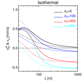
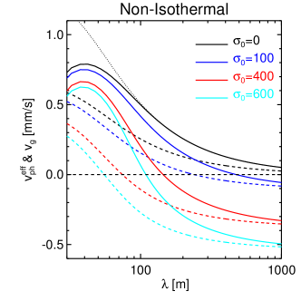
Figure 27: Linear group velocity $v_{g}$ (solid curves) and the corresponding effective linear phase velocity $v_{ph}-\Omega/k$ (dashed curves) for the $\tau_{15}$-parameters with different surface densities $\sigma_{0}$(in units $\text{kg}\,\text{m}^{-2}$). The black dotted curve equals twice the effective phase velocity (black dashed curve) for the case $\sigma_{0}=0$. In a stroboscopic space-time diagram with a sampling of 1/orbit $v_{ph}^{\mbox{eff}}$ is the apparent phase velocity of wave structures.

Appendix B Additional Hydrodynamical Integrations

In this appendix we briefly describe hydrodynamical integrations which address specific topics that were pointed out in Section 6.1.

B.1 Influence of the Radial Domain Size on the Saturation Wavelength

In Section 6.1 we noted that for very small surface mass densities $\sigma_{0}$ the finite size of the computational domain limits the growth of large-scale structures in hydrodynamical integrations, thereby affecting the saturation wavelength $\lambda_{p}$. This limiting effect, demonstrated in Figure 28, becomes weaker with increasing $\sigma_{0}$. That is, for the $\tau_{15}$-parameters, a domain size of at least $L_{x}=30\,\text{km}$ is required for a surface density $\sigma_{0}=50\,\text{kg}\,\text{m}^{-2}$ (Figure 28 second column). Whereas, a size of $L_{x}=10\,\text{km}$ is sufficient for $\sigma_{0}=100\,\text{kg}\,\text{m}^{-2}$ (Figure 28 third column). Furthermore, for $\sigma_{0}\gtrsim 300\,\text{kg}\,\text{m}^{-2}$ a size $L_{x}=5\,\text{km}$ suffices to obtain a consistent value of the saturation wavelength [i.e. close to the value predicted by the empirical relation (55)].

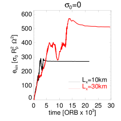
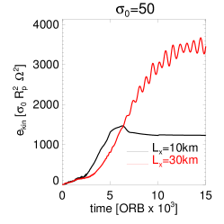
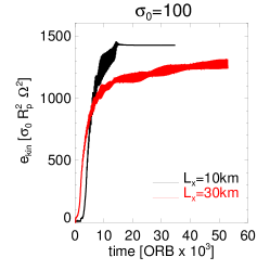
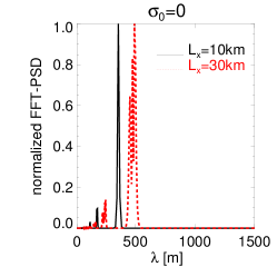
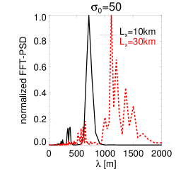
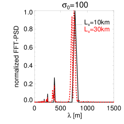
Figure 28: Illustration of the limiting effect of the size of calculation region $L_{x}$ on the evolution of the viscous overstability in hydrodynamic computations for small surface densities $\sigma_{0}$ ($\tau_{15}$-parameters). The upper three frames show the evolution of the kinetic energy densities and the lower frames the final power spectra for integrations with considerably different $L_{x}$. For the cases $\sigma_{0}=0$ and $\sigma_{0}=50\,\text{kg}\,\text{m}^{-2}$, the initial seed was equal (spectral white noise) for the two integrations with different $L_{x}$. For the integrations with $\sigma_{0}=100\,\text{kg}\,\text{m}^{-2}$ the initial conditions were a single wavelength mode $\lambda=100\,\text{m}$ ($L_{x}=10\,\text{km}$) and spectral white noise ($L_{x}=30\,\text{km}$).

B.2 Integrations with Modified Equation of State

Related to the discussion of Figures 5 and 22 (right panel), we performed several non-isothermal hydrodynamic integrations with the $\tau_{15}$-parameters and $L_{x}=10\,\text{km}$, employing the increased values of $p_{s}$ by factors of 1.4 and 2, mentioned in sections 4.2.2 and 6.1 (see also Figures 5 and 22). The result is that these modifications bring the saturation wavelength $\lambda_{p}$ for small surface densities $\sigma_{0}\leq 150\,\text{kg}\,\text{m}^{-2}$ very close to the value of $\lambda_{p}$ obtained for the case $\sigma_{0}=0$ with the original $p_{s}$ (with $L_{x}=10\,\text{km}$). Thus, a sufficiently large value of $p_{s}$ effectively removes the influence of the frequency minimum for small $\sigma_{0}$, by shifting it to very large wavelengths. Consequently, its approach is hindered by the size of the calculation region (Figure 28). However, the modified $p_{s}$ also leads to considerably increased values of $\lambda_{p}$ for larger surface densities $\sigma_{0}\gtrsim 300\,\text{kg}\,\text{m}^{-2}$, which makes the agreement with the N-body simulations worse.

B.3 Influence of the Initial State on the Saturation Wavelength

The saturation wavelengths of the hydrodynamic model (the asterisks in Figure 21) are obtained from integrations where the initial state consists of spectral white noise. In order to investigate possible saturation on alternative wavelengths (cf. Figure 23) we perform a series of integrations in a radial domain with $L_{x}=5-10\,\text{km}$, employing the $\tau_{15}$-parameters, where we seed a single wavelength large amplitude mode. As the seeded mode saturates, we follow the subsequent evolution for 10,000 orbits. In actual fact, we find for each surface density a whole range of wavelengths supporting stable traveling waves, not showing any signs of wavelength change for at least 10,000 orbits. For instance, for wavelengths $150\,\text{m}\lesssim\lambda\lesssim 250\,\text{m}$, all surface densities $\sigma_{0}\gtrsim 200\,\text{kg}\,\text{m}^{-2}$ support such stable traveling waves.

As speculated in Section 6.1, in some cases the smallness of the group velocity might explain the absence of changes of the wave train on the considered timescale. In other cases, however, the (quasi-)stability of single wavelength modes substantially different from those over-plotted in Figure 21, seems to contradict with N-body simulations, such as those in Figure 18 (left panel). As outlined before (Section 6.1), in N-body simulations numerous fluctuations due to the discrete nature of the particle flow are present at all times. These perturbations do not exist in the hydrodynamic model system, which might explain the resistance to change the dominant wavelength. When adding a buffer-zone in the computational domain though (cf. Sections 5.1.1 and 6.2), the system immediately responds. That is, it immediately excites power on a range of wavelengths located in close vicinity to the nonlinear frequency minimum. The power on these wavelengths subsequently increases and the prevalent wavelength approaches asymptotically a value close to the nonlinear frequency minimum (Section 6.2).

To illustrate this behavior, Figure 29 shows the evolution of the prevalent wavelengths and the kinetic energy densities of two integrations with $L_{x}=8\,\text{km}$ where modes with respective wavelengths $\lambda=125\,\text{m}$ and $\lambda=200\,\text{m}$ saturate and their evolution is followed for 10,000 orbits. At time $t=10,000\,\text{ORB}$ in both cases a buffer-zone is superimposed to the integration region such that $\beta<\beta_{c}$ for $x=[-0.5\,\text{km};0.5\,\text{km}]$. Also displayed is the evolution of an integration which started from low amplitude white noise and that included a buffer-zone from the beginning (cf. Section 6.2). As a result of the buffer-zone, in all of the three integrations source/sink structures form and the prevalent wavelength asymptotically approaches the nonlinear frequency minimum, which is marked by a horizontal dashed line in the left frame. In the integration which started from white noise the timescale for this approach is significantly shorter. Also, in the same integration, there are stronger fluctuations in $e_{kin}$ and $\lambda_{p}$, indicating stronger perturbations emitted by the source. These differences might be a consequence of the different source/sink configuration. In this integration a sink persists exterior to the buffer-zone so that the buffer-zone as a whole serves as a source. In contrast, the integrations starting from nonlinear unidirectional wave trains form source and sink structures within the buffer-zone so that the overall wave pattern effectively “tunnels” through the latter. Whether this difference is the reason for the different time scales is, however, speculative and should be addressed in future work. In this regard we like to note that the precise asymptotic behavior of these hydrodynamic integrations can depend slightly on the details of the applied numerical scheme, such as the reconstruction method used for the numerical flux vector (Section 4).

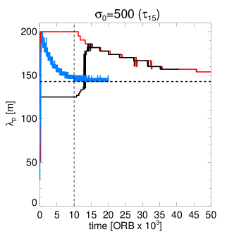
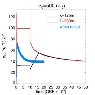
Figure 29: Two hydrodynamic integrations with $\sigma_{0}=500\,\text{kg}\,\text{m}^{-2}$ ($\tau_{15}$-parameters) started with different large amplitude single wavelength modes ($\lambda=125\,\text{m}$ and $\lambda=200\,\text{m}$, respectively) in a periodic domain with $L_{x}=8\,\text{km}$. Left and right panels show the prevalent wavelengths and kinetic energy densities for both integrations. The wave trains saturate rapidly and remain stable for at least 10,000 orbits. At time $t=10,000\,\text{ORB}$ (marked by the vertical dashed line) the integration regions are superimposed by a buffer-zone ($\beta=-0.5$ in the region $[-0.5\,\text{km};+0.5\,\text{km}]$). Note the sudden drop of $e_{kin}$ in these integrations at 10,000 orbits due to the buffer-zone. Also shown are $\lambda_{p}$ and $e_{kin}$ for an integration that started from white noise with a buffer-zone present at all times.

Appendix C Group Velocities of Saturated Wave Trains

In order to verify the computed nonlinear dispersion relations $\omega_{I}^{nl}(k)$ (Figure 21 in Section 6.1) of overstable waves, we can compare the propagation speed of small perturbations imposed to saturated wave trains with the group velocity $\mathrm{d}\omega_{I}^{nl}(k)/\mathrm{d}k$, obtained by numerical differentiation. Figure 30 presents space-time diagrams of saturated (left) traveling waves resulting from integrations with the $\tau_{15}$-parameters which started from white noise. Frame (a) shows the same integration as in Figure 11. Frames (b) and (e) are the same integrations as in Figure 14. The primary waves in each frame correspond to the small scale structure. Perturbations in the wave amplitudes are visible on much larger scale and develop in all cases in the course of the nonlinear evolution. The red lines represent the group velocities computed by numerical differentiation (using 3-point Lagrangian interpolation) of the measured nonlinear frequency curves in Figure 21a at the corresponding saturation wavelengths (the asterisks) for each $\sigma_{0}$ (units $\text{kg}\,\text{m}^{-2}$). The values of $v_{g}$ are indicated for all cases, matching well the propagation of the long wavelength undulations.

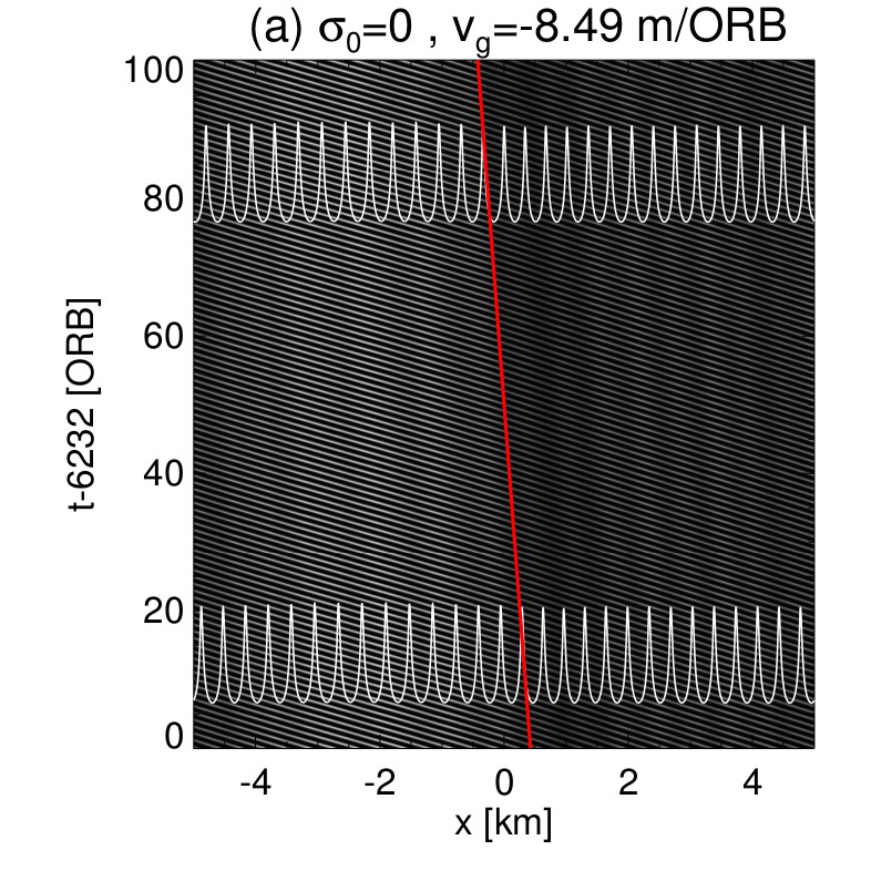
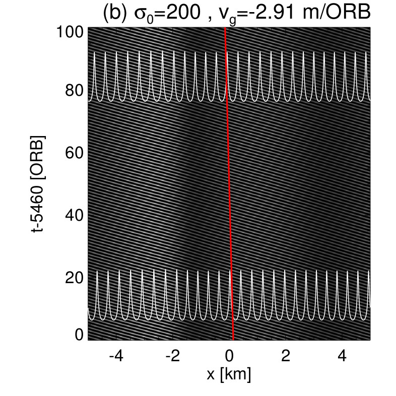
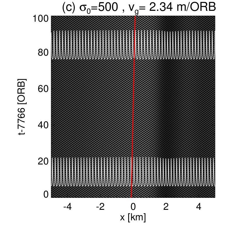
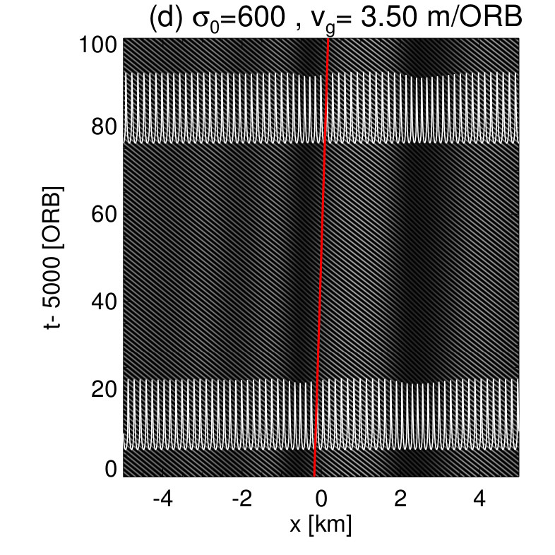
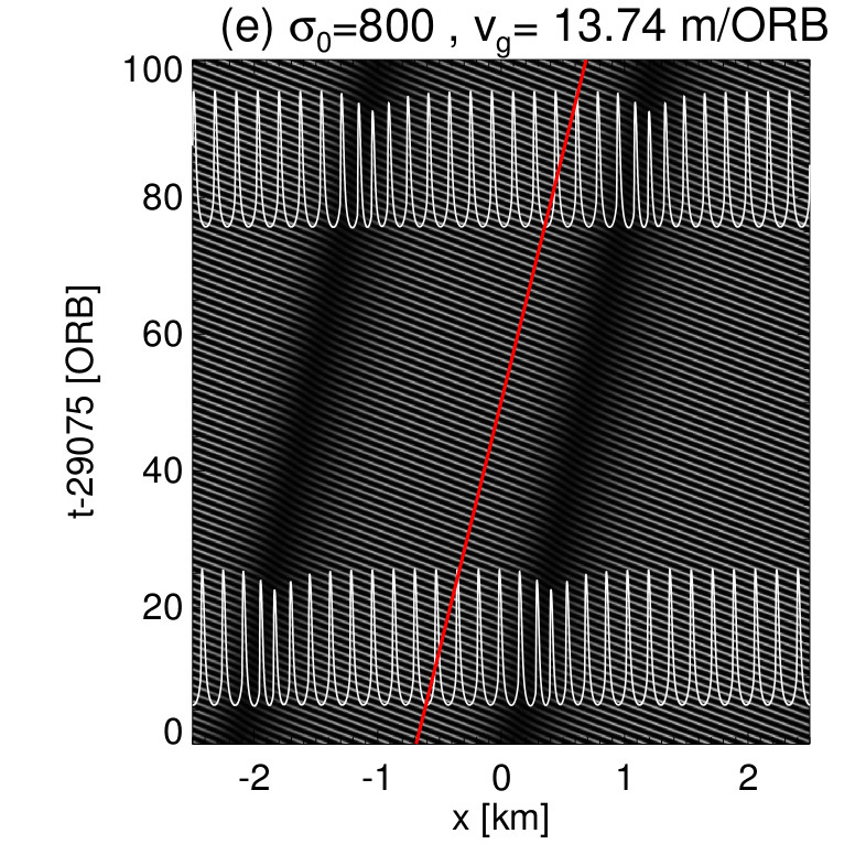
Figure 30: Space-time diagrams of saturated traveling waves resulting from integrations with the $\tau_{15}$-parameters. The movement of long wavelength undulations occurs with the group velocity of the wave train which is indicated by red lines. Also shown in each frame are the profiles of surface mass density (enhanced by a factor of 10) corresponding to early and late stages of the displayed evolution. See the text for more explanation.

References

- Araki and Tremaine, (1986) Araki, S. and Tremaine, S. (1986). The dynamics of dense particle disks. Icarus, 65:83–109.
- Ballouz et al., (2017) Ballouz, R.-L., Richardson, D. C., and Morishima, R. (2017). Numerical Simulations of Saturn’s B Ring: Granular Friction as a Mediator between Self-gravity Wakes and Viscous Overstability. AJ, 153:146.
- Binney and Tremaine, (1987) Binney, J. and Tremaine, S. (1987). Galactic Dynamics. Princeton University Press.
- Borderies et al., (1985) Borderies, N., Goldreich, P., and Tremaine, S. (1985). A granular flow model for dense planetary rings. Icarus, 63:406–420.
- Bridges et al., (1984) Bridges, F., Hatzes, A., and Lin, D. (1984). Structure, stability and evolution of Saturn’s rings. Nature, 309:333–338.
- Chapman and Cowling, (1970) Chapman, S. and Cowling, T. (1970). The mathematical theory of non-uniform gases. Cambridge University Press, Cambridge.
- Colwell et al., (2007) Colwell, J. E., Esposito, L. W., Sremčević, M., Stewart, G. R., and McClintock, W. E. (2007). Self-gravity wakes and radial structure of Saturn’s B ring. Icarus, 190:127–144.
- Colwell et al., (2009) Colwell, J. E., Nicholson, P. D., Tiscareno, M. S., Murray, C. D., French, R. G., and Marouf, E. A. (2009). The Structure of Saturn’s Rings, page 375.
- Daisaka et al., (2001) Daisaka, H., Tanaka, H., and Ida, S. (2001). Viscosity in a dense planetary ring with self-gravitating particles. Icarus.
- Dilley, (1993) Dilley, J. P. (1993). Energy loss in collision of icy spheres: Loss mechanism and size-mass dependence. Icarus, 105:225–234.
- French et al., (2007) French, R. G., Salo, H., McGhee, C. A., and Dones, L. (2007). HST observations of azimuthal asymmetry in Saturn’s rings. Icarus, 189:493–522.
- Goldreich and Lynden-Bell, (1965) Goldreich, P. and Lynden-Bell, D. (1965). II. Spiral arms as sheared gravitational instabilities. mnras, 130:125.
- Goldreich and Tremaine, (1978) Goldreich, P. and Tremaine, S. (1978). The velocity dispersion in Saturn’s rings. Icarus, 34:227–239.
- Gottlieb et al., (2001) Gottlieb, S., Shu, C.-W., and Tadmor, E. (2001). Strong Stability-Preserving High-Order Time Discretization Methods. SIAM Review, 43:89–112.
- Haff, (1983) Haff, P. K. (1983). Grain flow as a fluid–mechanical phenomenon. J. Fluid Mech., 134:401–430.
- Hämeen-Anttila and Salo, (1993) Hämeen-Anttila, K. A. and Salo, H. (1993). Generalized Theory of Impacts in Particulate Systems. Earth Moon and Planets, 62:47–84.
- Hedman and Nicholson, (2016) Hedman, M. M. and Nicholson, P. D. (2016). The B-ring’s surface mass density from hidden density waves: Less than meets the eye? Icarus, 279:109–124.
- Hedman et al., (2014) Hedman, M. M., Nicholson, P. D., and Salo, H. (2014). Exploring Overstabilities in Saturn’s A Ring Using Two Stellar Occultations. AJ, 148:15.
- Hedman et al., (2007) Hedman, M. M., Nicholson, P. D., Salo, H., Wallis, B. D., Buratti, B. J., Baines, K. H., Brown, R. H., and Clark, R. N. (2007). Self-Gravity Wake Structures in Saturn’s A Ring Revealed by Cassini VIMS. AJ, 133:2624–2629.
- Hwang and Hutter, (1995) Hwang, H. and Hutter, K. (1995). A new kinetic model for rapid granular flow. Continuum Mechanics and Thermodynamics, 7:357–384.