Extrofitting: Enriching Word Representation and its Vector Space
with Semantic Lexicons

Abstract

We propose post-processing method for enriching not only word representation but also its vector space using semantic lexicons, which we call extrofitting. The method consists of 3 steps as follows: (i) Expanding 1 or more dimension(s) on all the word vectors, filling with their representative value. (ii) Transferring semantic knowledge by averaging each representative values of synonyms and filling them in the expanded dimension(s). These two steps make representations of the synonyms close together. (iii) Projecting the vector space using Linear Discriminant Analysis, which eliminates the expanded dimension(s) with semantic knowledge. When experimenting with GloVe, we find that our method outperforms Faruqui’s retrofitting on some of word similarity task. We also report further analysis on our method in respect to word vector dimensions, vocabulary size as well as other well-known pretrained word vectors (e.g., Word2Vec, Fasttext).

1 Introduction

As a method to represent natural language on computer, researchers have utilized distributed word representation. The distributed word representation is to represent a word as n-dimensional float vector, hypothesizing that some or all of the dimensions may capture semantic meaning of the word. The representation has worked well in various NLP tasks, substituting one-hot representation Turian et al. (2010). Two major algorithms learning the distributed word representation are CBOW (Continuous Bag-of-Words) and skip-gram Mikolov et al. (2013b). Both CBOW and skip-gram learn the representation using one hidden neural networks. The difference is that CBOW learns the representation of a center word from neighbor words whereas skip-gram gets the representation of neighbor words from a center word. Therefore, the algorithms have to depend on word order, because their objective function is to maximize the probability of occurrence of neighbor words given the center word. Then a problem occurs because the word representations do not have any information to distinguish synonyms and antonyms. For example, worthy and desirable should be mapped closely on the vector space as well as agree and disagree should be mapped apart, although they occur on a very similar pattern. Researchers have focused on the problem, and their main approaches are to use semantic lexicons Faruqui et al. (2014); Mrkšić et al. (2016); Speer et al. (2017); Vulić et al. (2017); Camacho-Collados et al. (2015). One of the successful works is Faruqui’s retrofitting, which can be summarized as pulling word vectors of synonyms close together by weighted averaging the word vectors on a fixed vector space (it will be explained in Section 2.1). The retrofitting greatly improves word similarity between synonyms, and the result not only corresponds with human intuition on words but also performs better on document classification tasks with comparison to original word embeddings Kiela et al. (2015). From the idea of retrofitting, our method hypothesize that we can enrich not only word representation but also its vector space using semantic lexicons. We call our method as extrofitting, which retrofits word vectors by expanding its dimensions.

2 Backgrounds

2.1 Retrofitting

Retrofitting Faruqui et al. (2014) is a post-processing method to enrich word vectors using synonyms in semantic lexicons. The algorithm learns the word embedding matrix $Q=\{q_{1},q_{2},\dots,q_{n}\}$ with the objective function $\Psi(Q)$:

$$\Psi(Q)=\sum_{i=1}^{n}\ [\alpha||q_{i}-\hat{q}_{i}||^{2}+\sum_{(i,j)\in E}\beta_{ij}||q_{i}-q_{j}||^{2}]$$ (1)

where an original word vector is ${q}_{i}$, its synonym vector is $q_{j}$, and inferred word vector is $\hat{q}_{i}$. The hyperparameter $\alpha$ and $\beta$ control the relative strengths of associations. The $\hat{q}_{i}$ can be derived by the following online update: $\hat{q}_{i}=\frac{\sum_{j:(i,j)\in E}\beta_{ij}q_{j}+\alpha_{i}q_{i}}{\sum_{j:(i,j)\in E}\beta_{ij}+\alpha_{i}}$

2.2 Linear Discriminant Analysis (LDA)

LDA Welling (2005) is one of the dimension reduction algorithms that project data into different vector space, while minimizing the loss of class information as much as possible. As a result, the algorithm finds linear vector spaces which minimize the distance of data in the same class as well as maximize the distance among the different class. The algorithm can be summarized as follows:
Calculating between-class scatter matrix $S_{B}$ and within-class scatter matrix $S_{W}$.
When we denote data as $x$, classes as $c$, $S_{B}$ and $S_{W}$ can be formulated as follows:

$$S_{B}=\sum_{c}(\mu_{i}-\mu)(\mu_{i}-\mu)^{T},$$ (2)

$$S_{W}=\sum_{c}\sum_{i\in c}(x_{i}-\mu_{c})(x_{i}-\mu_{c})^{T},$$ (3)

where the overall average of $x$ is $\mu$, and the partial average in class $i$ is denoted by $\mu_{i}$.
Maximizing the objective function $J(w)$.
The objective function $J(w)$ that we should maximize can be defined as

$$J(w)=\frac{|U^{T}S_{B}U|}{|U^{T}S_{W}U|},$$ (4)

and its solution can be reduced to find U that satisfies $S_{W}^{-1}S_{B}=U\Lambda U^{T}.$ Therefore, $U$ is derived by eigen-decomposition of $S_{W_{i}}^{-1}S_{B}$; choosing $q$ eigen vectors which have the top-$q$ eigen values, and composing transform matrix of $U$.
Transforming data onto new vector space
Using transform matrix $U$, we can get transformed data by $y=U^{T}x$

3	MEN-3k	WS353	SL-999	RG-65	#Extrofitted	#Vocab.
3 glove.6B.300d	0.7486	0.5170	0.3705	0.7693	-	0.4M
+ PPDB	0.7949	0.5826	0.4387	0.8177	67,729	-
+ WordNetsyn	0.7884	0.5805	0.4409	0.7943	55,388	-
+ WordNetall	0.7893	0.5714	0.4353	0.8010	55,388	-
+ FrameNet	0.7840	0.5837	0.4376	0.8187	7,592	-
2 glove.42B.300d	0.7435	0.5516	0.3738	0.8172	-	1.9M
+ PPDB	0.8292	0.6613	0.4896	0.8362	76,631	-
+ WordNetsyn	0.8230	0.6605	0.4884	0.8634	70,411	-
+ WordNetall	0.8223	0.6638	0.4858	0.8561	70,411	-
+ FrameNet	0.8123	0.6448	0.4601	0.8556	7,809	-
3

Table 1: Spearman’s correlation of extrofitted word vectors for word similarity tasks using semantic lexicon. Our method improves pretrained GloVe in different vocabulary size.

3 Enriching Representations of Word Vector and The Vector Space

3.1 Expanding Word Vector with Enrichment

We simply enrich the word vectors by expanding dimension(s) that add 1 or more dimension to original vectors, filling with its representative value $r_{i}$, which can be a mean value. We denote an original word vectors as $q_{i}=(e_{1},e_{2},\cdots,e_{D})$ where D denotes the number of word vector dimension. Then, the representative value $r_{i}$ can be formulated as $r_{i}=mean(e_{1},e_{2},\cdots,e_{D})$. Intuitively, if we expand more additional dimensions, the word vectors will strengthen its own meaning. Likewise, the ratio of the number of expanded dimension to the number of original dimensions will affect the meaning of the word vectors.

3.2 Transferring Semantic Knowledge

To transfer semantic knowledge on the representative value $r_{i}$, we also take a simple approach of averaging all the representative values of each synonym pair, substituting each of its previous value. We get the synonym pairs from lexicons we introduced in Section 3. The transferred representative value $\bar{r}_{i}$ can be formulated as $\bar{r}_{i}=\sum_{s\in L}r_{s}/N$ where L refers to the lexicon consisting of synonym pairs $s$, and $N$ is the number of synonyms. This manipulation makes the representation of the synonym pairs close to one another.

3.3 Enriching Vector Space

With the enriched vectors and the semantic knowledge, we perform Linear Discriminant Analysis for dimension reduction as well as clustering the synonyms from semantic knowledge. LDA finds new vector spaces to cluster and differentiate the labeled data, which are synonym pairs in this experiment. We can get the extrofitted word embedding matrix $\bar{w}$ as follows:

$$\bar{Q}=\textit{LDA}(Q\oplus\bar{r},l)$$ (5)

where $Q$ is the word embedding matrix composed of word vectors $q$ and $l$ is the index of the synonym pair. We implement our method using Python2.7 with scikit-learn Pedregosa et al. (2011).

4 Experiment Data

4.1 Pretrained Word Vectors

GloVe Pennington et al. (2014) has lots of variations in respect to word dimension, number of tokens, and train sources. We used glove.6B trained on Wikipedia+Gigawords and glove.42B.300d trained on Common Crawl. The other pretrained GloVe do not fit in our experiment because they have different word dimension or are case-sensitive. We also use 300-dimensional Word2Vec Mikolov et al. (2013a) with negative sampling trained on GoogleNews corpus. Fasttext Bojanowski et al. (2016) is an extension of Word2Vec, which utilizes subword information to represent an original word. We used 300-dimensional pretrained Fasttext trained on Wikipedia (wiki.en.vec), using skip-gram.

4.2 Semantic Lexicons

We borrow the semantic lexicons from retrofitting Faruqui et al. (2014). Faruqui et al. extracted the synonyms from PPDB Ganitkevitch et al. (2013) by finding a word that more than two words in another language are corresponding with. Retrofitting also used WordNet Miller (1995) database which grouped words into set of synonyms (synsets). We used two versions of WordNet lexicon, one which consists of synonym only (WordNet_syn) and the other with additional hypernyms, hyponyms included (WordNet_all). Lastly, synonyms were extracted from FrameNet Baker et al. (1998), which contains more than 200,000 manually annotated sentences linked to semantic frames. Faruqui et al. regarded words as synonyms if the words can be grouped with any of the frames.

4.3 Evaluation Data

We evaluate our methods on word similarity tasks using 4 different kinds of dataset. MEN-3k Bruni et al. (2014) consists of 3000-word pairs rated from 0 to 50. WordSim-353 Finkelstein et al. (2001) consists of 353-word pairs rated from 0 to 10. SimLex-999 Hill et al. (2015) includes 999-word pairs rated from 0 to 10. RG-65 Rubenstein and Goodenough (1965) has 65 words paired scored from 0 to 4. MEN-3k and WordSim-353 were split into train (or dev) set and test set, but we combined them together solely for evaluation purpose. The other datasets have lots of out-of-vocabulary, so we disregard them for future work.

3	MEN-3k	WS353	SL-999	RG-65	Lexicon
3 glove.6B.50d	0.6574	0.4193	0.2646	0.5948	-
+ Retrofitting	0.6773	0.4121	0.3761	0.7027	WordNetall
+ Extrofitting	0.6876	0.4859	0.2926	0.6743	WordNetall
2 glove.6B.100d	0.6932	0.4488	0.2975	0.6762	-
+ Retrofitting	0.7052	0.4428	0.4065	0.7863	WordNetall
+ Extrofitting	0.7447	0.5337	0.3733	0.7341	WordNetall
2 glove.6B.200d	0.7244	0.4866	0.3403	0.7128	-
+ Retrofitting	0.7397	0.4799	0.4415	0.8123	WordNetall
+ Extrofitting	0.7689	0.5416	0.4120	0.7389	WordNetall
2 glove.6B.300d	0.7486	0.5130	0.3705	0.7693	-
+ Retrofitting	0.7681	0.5232	0.4701	0.8499	WordNetall
+ Extrofitting	0.7893	0.5714	0.4353	0.8010	WordNetall
3

Table 2: Comparison of Spearman’s correlation of retrofitted or extrofitted word vectors for word similarity tasks. Our method, extrofitting, outperforms retrofitting on MEN-3k and WordSim-353.

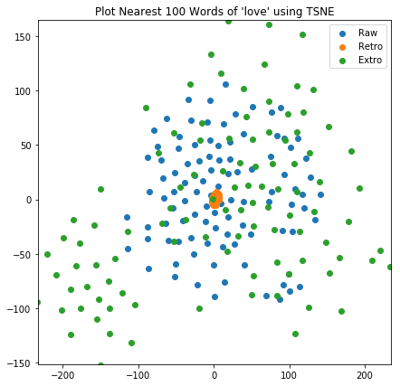
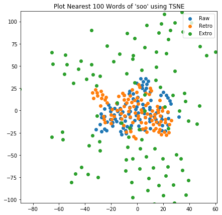
Figure 1: Plots of nearest top-100 words of cue words in different post-processing methods. We choose two cue words; one is included in semantic lexicons (love; left), and another is not (soo; right)

3 Cue Word	Method	Top-10 Nearest Words(Cosine Similarity Score)
3 love	glove.42B.300d	loved(.7745), i(.7338), loves(.7311), know(.7286), loving(.7263), really(.7196), always(.7193), want(.7192), hope(.7127), think(.7110)
	+ Retrofitting	loved(.7857), know(.7826), like(.7781), want(.7736), i(.7707), feel(.7549), wish(.7549), think(.7491), enjoy(.7453), loving(.7451)
	+ Extrofitting	loved(.6008), adore(.5949), hate(.5949), luv(.5562), loving(.5391), loooove(.5321), looooove(.5233), loveeee(.5195), want(.5171), looove(.5107)
soo	glove.42B.300d	sooo(.8394), soooo(.7938), sooooo(.7715), soooooo(.7359), sooooooo(.6844), haha(.6574), hahah(.6320), damn(.6247), omg(.6244), hahaha(.6219)
	+ Retrofitting	sooo(.8394), soooo(.7938), sooooo(.7715), soooooo(.7359), haha(.6574), hahah(.6320), omg(.6244), hahaha(.6219), sooooooo(.6189)
	+ Extrofitting	sooo(.8329), soooo(.7896), sooooo(.7774), soooooo(.7560), sooooooo(.7256), soooooooo(.6867), sooooooooo(.6796), soooooooooo(.6517), tooo(.6493), sooooooooooo(.6423)
3

Table 3: List of top-10 nearest words of cue words in different post-processing methods. We show cosine similarity scores of two words included in semantic lexicon (love) or not (soo).

3	MEN-3k	WS353	SL-999	RG-65	#Extrofitted	#Vocab.
3 w2v-google-news	0.7764	0.6156	0.4475	0.7558	-	3.0M
+ PPDB	0.7883	0.5935	0.4799	0.7877	63,825	-
+ WordNetsyn	0.7821	0.6004	0.4741	0.7844	64,248	-
+ WordNetall	0.7782	0.6051	0.4733	0.7782	64,248	-
+ FrameNet	0.7784	0.6025	0.4651	0.7650	7,559	-
2 wiki.en.vec	0.7654	0.6301	0.3803	0.8005	-	2.5M
+ PPDB	0.7737	0.6363	0.4133	0.7723	69,237	-
+ WordNetsyn	0.7599	0.6326	0.4135	0.7633	70,542	-
+ WordNetall	0.7569	0.6421	0.4093	0.7459	70,542	-
+ FrameNet	0.7594	0.6323	0.4051	0.7740	7,637	-
3

Table 4: Spearman’s correlation of extrofitted word vectors for word similarity tasks on pretrained word vectors by Word2Vec and Fasttext. Extrofitting can be applied to other kinds of pretrained word vector.

5 Experiments on Word Similarity Task

The word similarity task is to calculate Spearman’s correlation Daniel (1990) between two words as word vector format. We first apply extrofitting to GloVe from different data sources and present the result in Table 1. The result shows that although the number of the extrofitted word with FrameNet is less than the other lexicons, its performance is on par with other lexicons. We can also ensure that our method improves the performance of original pretrained word vectors.
Next, we perform extrofitting on GloVe in different word dimension and compare the performance with retrofitting. We use WordNet_all lexicon on both retrofitting and extrofitting to compare the performances in the ideal environment for retrofitting. We present the results in Table 2. We can demonstrate that our method outperforms retrofitting on some of word similarity tasks, MEN-3k and WordSim-353. We believe that extrofitting on SimLex-999 and RG-65 is less powerful because all word pairs in the datasets are included on WordNet_all lexicon. Since retrofitting forces the word similarity to be improved by weighted averaging their word vectors, it is prone to be overfitted on semantic lexicons. On the other hand, extrofitting also uses synonyms to improve word similarity but it works differently that extrofitting projects the synonyms both close together on a new vector space and far from the other words. Therefore, our method can make more generalized word representation than retrofitting. We plot top-100 nearest words using t-SNE Maaten and Hinton (2008), as shown in Figure 1. We can find that retrofitting strongly collects synonym words together whereas extrofitting weakly disperses the words, resulting loss in cosine similarity score. However, the result of extrofitting can be interpreted as generalization that the word vectors strengthen its own meaning by being far away from each other, still keeping synonyms relatively close together (see Table 3). When we list up top-10 nearest words, extrofitting shows more favorable results than retrofitting. We can also observe that extrofitting even can be applied to words which are not included in semantic lexicons.
Lastly, we apply extrofitting to other well-known pretrained word vectors trained by different algorithms (see Subsection 4.1). The result is presented in Table 4. Extrofitting can be also applied to Word2Vec and Fasttext, enriching their word representations except on WordSim-353 and RG-65, respectively. We find that our method can distort the well-established word embeddings. However, our results are noteworthy in that extrofitting can be applied to other kinds of pretrained word vectors for further enrichment.

6 Conclusion

We propose post-processing method for enriching not only word representation but also its vector space using semantic lexicons, which we call extrofitting. Our method takes a simple approach that (i) expanding word dimension (ii) transferring semantic knowledge on the word vectors (iii) projecting the vector space with enrichment. We show that our method outperforms another post-processing method, retrofitting, on some of word similarity task. Our method is robust in respect to the dimension of word vector and the size of vocabulary, only including an explainable hyperparameter; the number of dimension to be expanded. Further, our method does not depend on the order of synonym pairs. As a future work, we will do further research about our method to generalize and improve its performance; First, we can experiment on other word similarity datasets for generalization. Second, we can also utilize Autoencoder Bengio et al. (2009) for non-linear projection with a constraint of preserving spatial information of each dimension of word vector.

References

- Baker et al. (1998) Collin F Baker, Charles J Fillmore, and John B Lowe. 1998. The berkeley framenet project. In Proceedings of the 17th international conference on Computational linguistics-Volume 1, pages 86–90. Association for Computational Linguistics.
- Bengio et al. (2009) Yoshua Bengio et al. 2009. Learning deep architectures for ai. Foundations and trends® in Machine Learning, 2(1):1–127.
- Bojanowski et al. (2016) Piotr Bojanowski, Edouard Grave, Armand Joulin, and Tomas Mikolov. 2016. Enriching word vectors with subword information. arXiv preprint arXiv:1607.04606.
- Bruni et al. (2014) Elia Bruni, N Tram, Marco Baroni, et al. 2014. Multimodal distributional semantics. The Journal of Artificial Intelligence Research, 49:1–47.
- Camacho-Collados et al. (2015) José Camacho-Collados, Mohammad Taher Pilehvar, and Roberto Navigli. 2015. Nasari: a novel approach to a semantically-aware representation of items. In Proceedings of the 2015 Conference of the North American Chapter of the Association for Computational Linguistics: Human Language Technologies, pages 567–577.
- Daniel (1990) Wayne W Daniel. 1990. Spearman rank correlation coefficient. Applied nonparametric statistics, pages 358–365.
- Faruqui et al. (2014) Manaal Faruqui, Jesse Dodge, Sujay K Jauhar, Chris Dyer, Eduard Hovy, and Noah A Smith. 2014. Retrofitting word vectors to semantic lexicons. arXiv preprint arXiv:1411.4166.
- Finkelstein et al. (2001) Lev Finkelstein, Evgeniy Gabrilovich, Yossi Matias, Ehud Rivlin, Zach Solan, Gadi Wolfman, and Eytan Ruppin. 2001. Placing search in context: The concept revisited. In Proceedings of the 10th international conference on World Wide Web, pages 406–414. ACM.
- Ganitkevitch et al. (2013) Juri Ganitkevitch, Benjamin Van Durme, and Chris Callison-Burch. 2013. Ppdb: The paraphrase database. In Proceedings of the 2013 Conference of the North American Chapter of the Association for Computational Linguistics: Human Language Technologies, pages 758–764.
- Hill et al. (2015) Felix Hill, Roi Reichart, and Anna Korhonen. 2015. Simlex-999: Evaluating semantic models with (genuine) similarity estimation. Computational Linguistics, 41(4):665–695.
- Kiela et al. (2015) Douwe Kiela, Felix Hill, and Stephen Clark. 2015. Specializing word embeddings for similarity or relatedness. In Proceedings of the 2015 Conference on Empirical Methods in Natural Language Processing, pages 2044–2048.
- Maaten and Hinton (2008) Laurens van der Maaten and Geoffrey Hinton. 2008. Visualizing data using t-sne. Journal of machine learning research, 9(Nov):2579–2605.
- Mikolov et al. (2013a) Tomas Mikolov, Kai Chen, Greg Corrado, and Jeffrey Dean. 2013a. Efficient estimation of word representations in vector space. arXiv preprint arXiv:1301.3781.
- Mikolov et al. (2013b) Tomas Mikolov, Ilya Sutskever, Kai Chen, Greg S Corrado, and Jeff Dean. 2013b. Distributed representations of words and phrases and their compositionality. In Advances in neural information processing systems, pages 3111–3119.
- Miller (1995) George A Miller. 1995. Wordnet: a lexical database for english. Communications of the ACM, 38(11):39–41.
- Mrkšić et al. (2016) Nikola Mrkšić, Diarmuid O Séaghdha, Blaise Thomson, Milica Gašić, Lina Rojas-Barahona, Pei-Hao Su, David Vandyke, Tsung-Hsien Wen, and Steve Young. 2016. Counter-fitting word vectors to linguistic constraints. arXiv preprint arXiv:1603.00892.
- Pedregosa et al. (2011) F. Pedregosa, G. Varoquaux, A. Gramfort, V. Michel, B. Thirion, O. Grisel, M. Blondel, P. Prettenhofer, R. Weiss, V. Dubourg, J. Vanderplas, A. Passos, D. Cournapeau, M. Brucher, M. Perrot, and E. Duchesnay. 2011. Scikit-learn: Machine learning in Python. Journal of Machine Learning Research, 12:2825–2830.
- Pennington et al. (2014) Jeffrey Pennington, Richard Socher, and Christopher Manning. 2014. Glove: Global vectors for word representation. In Proceedings of the 2014 conference on empirical methods in natural language processing (EMNLP), pages 1532–1543.
- Rubenstein and Goodenough (1965) Herbert Rubenstein and John B Goodenough. 1965. Contextual correlates of synonymy. Communications of the ACM, 8(10):627–633.
- Speer et al. (2017) Robert Speer, Joshua Chin, and Catherine Havasi. 2017. Conceptnet 5.5: An open multilingual graph of general knowledge. In AAAI, pages 4444–4451.
- Turian et al. (2010) Joseph Turian, Lev Ratinov, and Yoshua Bengio. 2010. Word representations: a simple and general method for semi-supervised learning. In Proceedings of the 48th annual meeting of the association for computational linguistics, pages 384–394. Association for Computational Linguistics.
- Vulić et al. (2017) Ivan Vulić, Nikola Mrkšić, and Anna Korhonen. 2017. Cross-lingual induction and transfer of verb classes based on word vector space specialisation. arXiv preprint arXiv:1707.06945.
- Welling (2005) Max Welling. 2005. Fisher linear discriminant analysis. Department of Computer Science, University of Toronto, 3(1).