Optimization of a plate with holes

Abstract

We consider a simply supported plate with constant thickness, defined on an unknown multiply connected domain. We optimize its shape according to some given performance functional. Our method is of fixed domain type, easy to be implemented, based on a fictitious domain approach and the control variational method. The algorithm that we introduce is of gradient type and performs simultaneous topological and boundary variations. Numerical experiments are also included and show its efficiency.

1 Introduction

Shape optimization or optimal design is now a well established branch of the calculus of variations. It is a development of the optimal control theory with the minimization parameter being just the domain where the problem is defined. Basic references in this respect are Pironneau [16], Sokolowski, Zolesio [19], Delfour, Zolesio [4], Neittaanmäki, Sprekels, Tiba [14], etc.

It is to be noted that the literature on shape optimization problems, including unknown or variable domains, is mainly devoted to second order elliptic equations. Concerning fourth order boundary value problems, for instance plate models, there are papers Kawohl, Lang [8], Muñoz, Pedregal [11], Sprekels, Tiba [20], Arnautu, Langmach, Sprekels, Tiba[1] studying thickness optimization problems that may be reduced to optimal control problems by the coefficients. In Neittaanmäki, Sprekels, Tiba [14], Ch. VI, shape optimization problems for shells and curved rods, with constant thickness, are also studied. Since their parametric representation of the geometric form enters into the coefficients of the model, the shape optimization problems are again formulated as optimal control problems by the coefficients.

It is the aim of this work to extend the study of the optimization and the approximation for variable/unknown domain problems, from the case of second order elliptic operators, to fourth order operators. The unknowns to be found are the position, the shape, the size, the number of the holes defining the optimal plate and the given thickness is assumed constant. The main tools that we use is the fictitious domain approach Neittaanmäki, Pennanen, Tiba [13], Neittaanmäki, Tiba [15], Halanay, Murea, Tiba [6], Murea, Tiba [12] and the control variational method, Barboteu, Sofonea, Tiba [2], Sofonea, Tiba [18], Neittaanmäki, Sprekels, Tiba [14] and their references.

The plan of the work is as follows. In the next section we discuss the plate model that we take into account and its approximation via the fictitious domain method, under weak regularity assumptions on the geometry. This is important from the point of view of the associated shape optimization problems since it ensures a large class of admissible domains. Section 3 is devoted to the analysis of such optimal design problems, including their gradient and a general gradient-type algorithm, for their solution. In the last section, numerical examples are investigated that show the capacity of our approach to generate simultaneous topological and boundary variations, in the geometric optimization process. Our results are discussed in $\mathbb{R}^{2}$ since this is the natural setting for plates, but extensions to higher dimension are possible.

2 The model and its approximation

Let $\Omega\subset\mathbb{R}^{2}$ be a bounded, smooth (multiply) connected open subset representing the shape of a plate of constant thickness (normalized to one). We consider the fourth order partial differential equation

$$\Delta\Delta y = f\hbox{ in }\Omega,$$ (2.1)

$$y = 0,\quad\Delta y=0\hbox{ on }\partial\Omega,$$ (2.2)

where $f\in L^{2}(\Omega)$ is the load and $y\in H^{4}(\Omega)\cap H^{1}_{0}(\Omega)$ is the vertical deflection of the plate. The existence, the regularity and the uniqueness of the strong solution of (2.1)-(2.2) is well known, under $\mathcal{C}^{1,1}$ conditions for $\partial\Omega$, [5].

The difficulty in the numerical solution of (2.1)-(2.2) is that the shape of $\Omega$ may be very complicated, if multiply connected, and the standard Finite Element Method (FEM) may be difficult to implement. Moreover, in the corresponding shape optimization problems, the geometry may change in each iteration in a complex way (simultaneous topological and boundary variations) and this is very costly to be handled by usual discretization methods.

We consider now another simply connected smooth bounded domain $D\subset\mathbb{R}^{2}$ such that $\Omega\subset D$ and define the following approximation of (2.1)-(2.2), in a sense to be made precise in the subsequent Proposition 2.1.

$$-\Delta y_{\epsilon}+\frac{1}{\epsilon}(1-H_{\Omega})y_{\epsilon} = z_{\epsilon}\hbox{ in }D,$$ (2.3)

$$y_{\epsilon} = 0\hbox{ on }\partial D,$$

$$-\Delta z_{\epsilon}+\frac{1}{\epsilon}(1-H_{\Omega})z_{\epsilon} = f\hbox{ in }D,$$ (2.4)

$$z_{\epsilon} = 0\hbox{ on }\partial D,$$

where $H_{\Omega}$ is the characteristic function of $\Omega$ in $D$. For the boundary value problems (2.3)-(2.4) we get in the standard way that the strong solutions satisfy $y_{\epsilon},z_{\epsilon}\in H^{2}(D)\cap H^{1}_{0}(D)$ if $D$ is in $\mathcal{C}^{1,1}$. Notice that the systems (2.3)-(2.4) arise from the application of both the control variational method and fictitious method, as mentioned in Section 1.

We relax now the regularity assumptions on the domain $\Omega$ and we suppose that it is of class $\mathcal{C}$ (the segment property, see [14], [21] ). In the boundary value problems (2.1)-(2.2) and (2.3)-(2.4) we shall work with weak solutions $y\in H^{2}(\Omega)\cap H^{1}_{0}(\Omega)$ and, respectively, $y_{\epsilon},z_{\epsilon}\in H^{1}_{0}(D)$.

Proposition 2.1

If $\Omega$ is of class $\mathcal{C}$, then $y_{\epsilon}|_{\Omega}\rightarrow y$ weakly in $H^{1}_{0}(\Omega)$ and strongly in $L^{2}(\Omega)$, where $y\in H^{2}(\Omega)\cap H_{0}^{1}(\Omega)$ satisfies (2.1)-(2.2) as a weak solution.

Proof. Multiply (2.4) by $z_{\epsilon}$ and integrate by parts:

$$\int_{D}|\nabla z_{\epsilon}|^{2}d\mathbf{x}+\frac{1}{\epsilon}\int_{D}(1-H_{\Omega})z_{\epsilon}^{2}d\mathbf{x}\leq\int_{D}f\,z_{\epsilon}\,d\mathbf{x}.$$ (2.5)

The Poincaré inequality and (2.5) gives $\{z_{\epsilon}\}$ bounded in $H^{1}_{0}(D)$ and $z_{\epsilon}\rightarrow\tilde{z}$ strongly in $L^{2}(D)$ and weakly in $H^{1}_{0}(D)$, on a subsequence. Moreover

$$\int_{D}(1-H_{\Omega})z_{\epsilon}^{2}d\mathbf{x}\rightarrow\int_{D\setminus\Omega}\tilde{z}^{2}d\mathbf{x}=0$$ (2.6)

due to (2.5) since $\{z_{\epsilon}\}$ is bounded in $L^{p}(D)$, $p\geq 1$ in dimension two and we also have $z_{\epsilon}\rightarrow\tilde{z}$ a.e. in $D$. One can use Lions’ lemma [9] to infer (2.6). By the Hedberg-Keldys stability property for domains of class $\mathcal{C}$ (see [14]) we obtain that $\tilde{z}\in H^{1}_{0}(\Omega)$.

The above arguments can be applied to (2.3) as well and we have $y_{\epsilon}\rightarrow\tilde{y}$ strongly in $L^{2}(D)$ and weakly in $H^{1}_{0}(D)$ and $\tilde{y}|_{\Omega}\in H^{1}_{0}(\Omega)$. Take any test function $\varphi\in\mathcal{C}^{\infty}_{0}(\Omega)$ and multiply (2.3), respectively (2.4). Since the supports are disjoint, the penalization terms in (2.3), (2.4) disappear and we get that $y_{\epsilon}$ satisfies (2.1) in the distribution sense. The boundary condition (2.2) are also satisfied due to the previous remarks. Since the limits $\tilde{y},\ \tilde{z}$ are unique, the convergence is in fact valid without taking subsequence. $\Box$

Consider now $H^{\epsilon}:D\rightarrow\mathbb{R}$ to be a $C^{1}$ regularization of the characteristic function $H_{\Omega}$ and $H^{\epsilon}\rightarrow H_{\Omega}$ strongly in $L^{p}(\Omega)$, $p\geq 1$. Examples of this type will be indicated in the next section.

Corollary 2.1

If in (2.3), (2.4) we replace $H_{\Omega}$ by $H^{\epsilon}$, the other notations being preserved, then the conclusion of Proposition 2.1 remains valid.

3 Shape optimization problems and their gradient

We associate to (2.1), (2.2) the following minimization problem

$$\min_{\Omega\in\mathcal{O}}\int_{\Lambda}J\left(\mathbf{x},y(\mathbf{x})\right)d\mathbf{x},$$ (3.1)

where $\mathcal{O}$ is the class of admissible domains to be defined below, $y\in H^{1}_{0}(\Omega)$ is the weak solution of (2.1), (2.2), $\Lambda$ may be $\Omega$ or $\partial\Omega$ or some part of $\Omega$ or $\partial\Omega$ and $J$ is the performance index of Carathéodory type (measurable in $\mathbf{x}$ and continuous in $y$). More hypotheses or constraints will be imposed as necessity appears. The problem (3.1), (2.1), (2.2) has a similar form with optimal control problems, however the optimization parameter here is the geometry, the domain $\Omega$ itself.

The family $\mathcal{O}$ should be “large” in order to perform the optimization in (3.1) on a consistent admissible class. We avoid regularity hypotheses on the geometry (that are frequently used in shape optimization, see [3], [16], [19]) and we have just assumed that any $\Omega\in\mathcal{O}$ is an open set of class $\mathcal{C}$, contained in some given bounded domain $D\subset\mathbb{R}^{2}$:

$$\Omega\subset D,\quad\forall\Omega\in\mathcal{O}.$$ (3.2)

On may add the constraint

$$E\subset\Omega,\quad\forall\Omega\in\mathcal{O}$$ (3.3)

where $E\subset\subset D$ is some given not empty subset of $\mathbb{R}^{2}$.

Let $X(D)$ denote a subset of $\mathcal{C}(\overline{D})$. For instance, $X(D)$ may be a finite element space defined in $D$. Following [13], [15], with any $g\in X(D)$, that we call a parametrization of the geometry, we associate the open set

$$\Omega_{g}=int\left\{\mathbf{x}\in D;\ g(\mathbf{x})\geq 0\right\}.$$ (3.4)

In the absence of regularity assumptions and due to the possible presence of critical points of $g$, it is possible that $g$ has level set $\{\mathbf{x}\in D;\ g(\mathbf{x})=k\}$ of positive measure. This is the reason for the form of the definition (3.4). This is, in principle, different from the set of points where $g(x)>0$. Notice that $\Omega_{g}$ is a Carathéodory open set, i.e. cracks or cuts are not allowed. However, high oscillations of the boundary are possible (and the segment property may not be always valid and has to be imposed separately). In general, $\Omega_{g}$ may have many connected components, that may be multiply connected. If constraint (3.3) is imposed, then $X(D)$ should include the condition:

$$g(\mathbf{x})\geq 0\hbox{ in }E.$$ (3.5)

If $H:\mathbb{R}\rightarrow\mathbb{R}$ denotes the maximal monotone extension of the Heaviside function (see [13], [10]) then $H(g)$ is the characteristic function of $\overline{\Omega}_{g}$. The regularization $H^{\epsilon}=H^{\epsilon}(g)$, from Corollary 2.1, can be simply obtained by a regularization of the Heaviside function. In [15], the following formula is used

$$H^{\epsilon}(r)=\left\{\begin{array}[]{ll}1-\frac{1}{2}e^{-\frac{r}{\epsilon}},&r\geq 0,\\ \frac{1}{2}e^{\frac{r}{\epsilon}},&r<0\end{array}\right.$$ (3.6)

but other choices are possible.

Taking into account the approximation results from the previous section, we approximate the minimization problem (3.1), (2.1), (2.2) by (3.1), (2.3), (2.4) where $H_{\Omega}$ is replaced by $H^{\epsilon}(g)$. The cost functional (3.1), depending on the form of $\Lambda$, may be approximated in the form

$$\int_{E}J\left(\mathbf{x},y_{\epsilon}(\mathbf{x})\right)d\mathbf{x},\quad\hbox{if }\Lambda=E,$$ (3.7)

$$\int_{D}H^{\epsilon}(g)J\left(\mathbf{x},y_{\epsilon}(\mathbf{x})\right)d\mathbf{x},\quad\hbox{if }\Lambda=\Omega.$$ (3.8)

The case $\Lambda=\partial\Omega$ imposes more regularity assumptions on the geometry in order to ensure the application of trace theorems and it has been recently discussed in Tiba [22] for second order operators. We limit our investigations here to (3.7), (3.8). The approximation of the state equation and of the cost functionals ensures that all the computations are to be performed in the fixed domains $E$ or $D$. The geometry $\Omega$ is hidden under this approach in the mapping $g\in X(D)$. Consequently, the approximating shape optimization problems are in fact optimal control problems with the control $g$ acting in the coefficients of the lowest order term in the differential operator. Notice as well the smooth dependence of $y_{\epsilon}$ on $g$ when $H^{\epsilon}$ is used instead of $H$. This is analyzed in the next result and is fundamental for the application of the gradient methods in the solution of the optimization problem (3.1), (2.1), (2.2).

Proposition 3.1

The mappings $g\rightarrow y_{\epsilon}=y_{\epsilon}(g)$, $g\rightarrow z_{\epsilon}=z_{\epsilon}(g)$ defined by (2.3), (2.4) with $H_{\Omega}$ replaced by $H^{\epsilon}(g)$ are Gâteaux differentiable between $\mathcal{C}(D)$ and $H^{1}_{0}(\Omega)$ and $w=\nabla y_{\epsilon}(g)v$, $u=\nabla z_{\epsilon}(g)v$ for any $v$ in $\mathcal{C}(D)$ satisfy the following system in variations:

$$-\Delta u+\frac{1}{\epsilon}(1-H^{\epsilon}(g))u = \frac{1}{\epsilon}(H^{\epsilon})^{\prime}(g)z_{\epsilon}v,$$

$$-\Delta w+\frac{1}{\epsilon}(1-H^{\epsilon}(g))w = u+\frac{1}{\epsilon}(H^{\epsilon})^{\prime}(g)y_{\epsilon}v,$$

with $u,w\in H^{1}_{0}(\Omega)$.

Proof. We denote by $y_{\epsilon}^{\lambda}=y_{\epsilon}(g+\lambda v)$, $z_{\epsilon}^{\lambda}=z_{\epsilon}(g+\lambda v)$, $\lambda\in\mathbb{R}$. Substrating the corresponding regularized equations and dividing by $\lambda\neq 0$, we get

$$-\Delta\frac{z_{\epsilon}^{\lambda}-z_{\epsilon}}{\lambda}+\frac{1}{\epsilon}(1-H^{\epsilon}(g+\lambda v))\frac{z_{\epsilon}^{\lambda}-z_{\epsilon}}{\lambda} = \frac{1}{\epsilon}\frac{H^{\epsilon}(g+\lambda v)-H^{\epsilon}(g)}{\lambda}z_{\epsilon},$$ (3.9)

$$-\Delta\frac{y_{\epsilon}^{\lambda}-y_{\epsilon}}{\lambda}+\frac{1}{\epsilon}(1-H^{\epsilon}(g+\lambda v))\frac{y_{\epsilon}^{\lambda}-y_{\epsilon}}{\lambda} = \frac{z_{\epsilon}^{\lambda}-z_{\epsilon}}{\lambda}$$ (3.10)

$$+\frac{1}{\epsilon}\frac{H^{\epsilon}(g+\lambda v)-H^{\epsilon}(g)}{\lambda}y_{\epsilon},$$

will null boundary conditions on $\partial D$ for $y_{\epsilon},z_{\epsilon},y_{\epsilon}^{\lambda},z_{\epsilon}^{\lambda}$. Here $\epsilon>0$ is fixed and $\lambda\in\mathbb{R}$ is the varying parameter ($\lambda\rightarrow 0$).

We multiply (3.9) by $\frac{z_{\epsilon}^{\lambda}-z_{\epsilon}}{\lambda}$ and, after some computations, we get

$$\int_{D}\left|\nabla\frac{z_{\epsilon}^{\lambda}-z_{\epsilon}}{\lambda}\right|^{2}d\mathbf{x}+\frac{1}{\epsilon}\int_{D}(1-H^{\epsilon}(g+\lambda v))\left|\frac{z_{\epsilon}^{\lambda}-z_{\epsilon}}{\lambda}\right|^{2}d\mathbf{x}$$

$$=\frac{1}{\epsilon}\int_{D}\frac{H^{\epsilon}(g+\lambda v)-H^{\epsilon}(g)}{\lambda}z_{\epsilon}\frac{z_{\epsilon}^{\lambda}-z_{\epsilon}}{\lambda}d\mathbf{x}.$$ (3.11)

Since $H^{\epsilon}$ is of class $\mathcal{C}^{1}$, we have $\frac{H^{\epsilon}(g+\lambda v)-H^{\epsilon}(g)}{\lambda}\rightarrow(H^{\epsilon})^{\prime}(g)v$ a.e. in $D$ and it is bounded in $L^{\infty}(D)$ with respect to $\lambda\in\mathbb{R}$. We get from (3.11) that $\left\{\frac{z_{\epsilon}^{\lambda}-z_{\epsilon}}{\lambda}\right\}$ is bounded in $H^{1}_{0}(D)$. On a subsequence, we have $\frac{z_{\epsilon}^{\lambda}-z_{\epsilon}}{\lambda}\rightarrow u\in H^{1}_{0}(D)$, weakly in $H^{1}_{0}(D)$ and strongly in $L^{2}(D)$.

A similar argument, using the boundedness of $\left\{\frac{z_{\epsilon}^{\lambda}-z_{\epsilon}}{\lambda}\right\}$ applied to (3.10), gives that $\left\{\frac{y_{\epsilon}^{\lambda}-y_{\epsilon}}{\lambda}\right\}$ is bounded in $H^{1}_{0}(D)$ and converges weakly in $H^{1}_{0}(D)$ and strongly in $L^{2}(D)$, to some limit $w\in H^{1}_{0}(D)$, on a subsequence. Passing to the limit in (3.9), (3.10) on a common subsequence, we get the equations from the proposition, satisfied by $u,w\in H^{1}_{0}(D)$.

We notice that the equations for $u$, $w$ have a unique solution and this shows that the above convergences are valid without taking subsequences. We conclude the Gâteaux differentiability of the maps $y_{\epsilon}(g)$, $z_{\epsilon}(g)$ and the proof is finished. $\Box$

We introduce now the so called adjoint system. To do this, we shall consider two cases of the cost functionals:

$$\frac{1}{2}\int_{E}(y_{\epsilon}-y_{d})^{2}d\mathbf{x},$$ (3.12)

which is a special case of (3.7) with some given $y_{d}\in L^{2}(D)$. The second functional is (3.8).

For the performance index (3.12), we introduce the following adjoint system

$$-\Delta p+\frac{1}{\epsilon}(1-H^{\epsilon}(g))p = \chi_{E}(y_{\epsilon}-y_{d})\hbox{ in }D,$$ (3.13)

$$-\Delta q+\frac{1}{\epsilon}(1-H^{\epsilon}(g))q = p\hbox{ in }D,$$ (3.14)

$$p=0,\quad q = 0\hbox{ on }\partial D,$$ (3.15)

where $\chi_{E}$ is the characteristic function of $E$ in $D$.

Proposition 3.2

The directional derivative of the cost functional (3.12) is given by

$$\frac{1}{\epsilon}\int_{D}(H^{\epsilon})^{\prime}(g)v(y_{\epsilon}p+z_{\epsilon}q)d\mathbf{x},$$

for $p,q$ satisfying (3.13)–(3.15) and for any $v\in\mathcal{C}(D)$.

Proof. We have (in the notations of Proposition 3.1):

$$L = \lim_{\lambda\rightarrow 0}\frac{1}{2\lambda}\left[\int_{E}(y_{\epsilon}^{\lambda}-y_{d})^{2}d\mathbf{x}-\int_{E}(y_{\epsilon}-y_{d})^{2}d\mathbf{x}\right]=\lim_{\lambda\rightarrow 0}\int_{E}\frac{y_{\epsilon}^{\lambda}-y_{\epsilon}}{\lambda}\,\frac{y_{\epsilon}^{\lambda}+y_{\epsilon}-2y_{d}}{2}d\mathbf{x}$$

$$= \int_{E}w(y_{\epsilon}-y_{d})d\mathbf{x}=\int_{D}w\left(-\Delta p+\frac{1}{\epsilon}(1-H^{\epsilon}(g))p\right)d\mathbf{x}$$

$$= \int_{D}p\left(-\Delta w+\frac{1}{\epsilon}(1-H^{\epsilon}(g))w\right)d\mathbf{x},$$

by (3.13) and the partial integration.

Using Proposition 3.1, we get:

$$L = \int_{D}p\left(u+\frac{1}{\epsilon}(H^{\epsilon})^{\prime}(g)y_{\epsilon}v\right)d\mathbf{x}$$

$$= \frac{1}{\epsilon}\int_{D}(H^{\epsilon})^{\prime}(g)y_{\epsilon}p\,v\,d\mathbf{x}+\int_{D}\left(-\Delta q+\frac{1}{\epsilon}(1-H^{\epsilon}(g))q\right)u\,d\mathbf{x}$$

$$= \frac{1}{\epsilon}\int_{D}(H^{\epsilon})^{\prime}(g)y_{\epsilon}p\,v\,d\mathbf{x}+\int_{D}\left(-\Delta u+\frac{1}{\epsilon}(1-H^{\epsilon}(g))u\right)q\,d\mathbf{x}$$

$$= \frac{1}{\epsilon}\int_{D}(H^{\epsilon})^{\prime}(g)y_{\epsilon}p\,v\,d\mathbf{x}+\frac{1}{\epsilon}\int_{D}(H^{\epsilon})^{\prime}(g)z_{\epsilon}q\,v\,d\mathbf{x}$$

by (3.14) and again by Proposition 3.1. This ends the proof. $\Box$

If the cost functional (3.8) is taken into account, the equation in variation is given by Proposition 3.1 as well, but in the adjoint system (3.13)–(3.15), the equation (3.13) has to be replaced by

$$-\Delta p+\frac{1}{\epsilon}(1-H^{\epsilon}(g))p=H^{\epsilon}(g)J_{y}^{\prime}(\mathbf{x},y_{\epsilon})v\hbox{ in }D,$$ (3.16)

under the differentiability assumption for $J(\mathbf{x},\cdot)$ and the $L^{2}(D)$ integrability for $J_{y}^{\prime}(\mathbf{x},y_{\epsilon})$. In a similar way, we get

Corollary 3.1

The directional derivative of the cost functional (3.8) has the form:

$$\int_{D}(H^{\epsilon})^{\prime}(g)\left[J(\mathbf{x},y_{\epsilon}(\mathbf{x}))+\frac{1}{\epsilon}\left(y_{\epsilon}(\mathbf{x})p(\mathbf{x})+z_{\epsilon}(\mathbf{x})q(\mathbf{x})\right)\right]v(\mathbf{x})\,d\mathbf{x}.$$

The first term in the above formula appears since in (3.8) the derivative of $H^{\epsilon}(g)$, for perturbation $g+\lambda v$, also appears.

Remark 3.1

By Proposition 3.2, the gradient of the performance index (3.12) is $\frac{1}{\epsilon}(H^{\epsilon})^{\prime}(g)(y_{\epsilon}p+z_{\epsilon}q)$ and the steepest descent direction is with minus sign. Another descent direction is $-(y_{\epsilon}p+z_{\epsilon}q)$ since the coefficient is positive due to the monotocity of $H^{\epsilon}(\cdot)$. It also has the advantage of simplicity. If polynomial regularizations of $H_{\Omega}$, like

$$\widetilde{H}^{\epsilon}(r)=\left\{\begin{array}[]{ll}1,&r\geq 0,\\ \frac{\epsilon(r+\epsilon)^{2}-2r(r+\epsilon)^{2}}{\epsilon^{3}},&-\epsilon<r<0,\\ 0,&r\leq-\epsilon\end{array}\right.$$

are used instead of (3.6), then the support of the gradient or of the steepest descent direction is in the set $\{-\epsilon<g(\mathbf{x})<0\}$, that is in a neighborhood of $\partial\Omega_{g}$ (when the roots of $g(\cdot)$ are noncritical). Similar considerations may be made in connection to the functional (3.8) and Corollary 3.1. Both variants of descent directions may generate boundary and/or topological variations of the domain $\Omega_{g}$. A more general situation is considered in the Proposition 4.1, in the next section.

As we have already mentioned, the shape optimization problem (3.1), (2.1), (2.2) may be approximated by (3.1), (2.3), (2.4). Using admissible domains defined in (3.4) and regularizations like (3.6) with approximation of the characteristic functions $H_{\Omega_{g}}$ by $H^{\epsilon}(g)$, we have to solve an optimal control problem with control $g\in X(D)$ acting in the lower order terms of the system. In particular, we also infer the necessary optimality conditions for the approximating control problem (3.1), (2.1), (2.2) with $H^{\epsilon}(g)$ instead of $H_{\Omega_{g}}$.

Corollary 3.2

Let $g_{\epsilon}^{*}\in X(D)$ denote an optimal solution. The optimality conditions for $g_{\epsilon}^{*}$ are given by the system (3.1), (2.3), (2.4), the adjoint system (3.13)–(3.15) (or (3.14)–(3.16) according to the form (3.12), respectively (3.8) of the cost) and the maximum principle:

$$\int_{D}(H^{\epsilon})^{\prime}(g_{\epsilon}^{*})(y_{\epsilon}^{*}p_{\epsilon}^{*}+z_{\epsilon}^{*}q_{\epsilon}^{*})v\,d\mathbf{x}\leq 0,\quad\forall v,$$

respectively

$$\int_{D}(H^{\epsilon})^{\prime}(g_{\epsilon}^{*})\left[J(\mathbf{x},y_{\epsilon}^{*}(\mathbf{x}))+\frac{1}{\epsilon}(y_{\epsilon}^{*}(\mathbf{x})p_{\epsilon}^{*}(\mathbf{x})+z_{\epsilon}^{*}(\mathbf{x})q_{\epsilon}^{*}(\mathbf{x}))\right]v(\mathbf{x})\,d\mathbf{x}\leq 0,\quad\forall v,$$

where $y_{\epsilon}^{*},z_{\epsilon}^{*}\in H^{1}_{0}(D)$ denote the approximating optimal states, $p_{\epsilon}^{*},q_{\epsilon}^{*}$ denote the corresponding adjoint states and $v\in\mathcal{C}(\overline{D})$ is any admissible variation such that $g_{\epsilon}^{*}+\lambda v\in X(D)$ for $\lambda>0$, small.

For instance, if $X(D)$ is given by (3.5), the admissible $v$ have to satisfy (3.5) as well.

By Proposition 3.2 and Corollary 3.1, gradient methods may be applied with various descent directions. We formulate the following general gradient with projection algorithm:

Algorithm 3.1

Step 1 Start with $n=0$, $\epsilon>0$ given “small” and select some initial $g_{n}$.

Step 2 Compute $y_{\epsilon}^{n},\ z_{\epsilon}^{n}$ the solution of (2.3), (2.4) with $H_{\Omega_{g}}$ replaced by $H^{\epsilon}(g)$.

Step 3 Compute $p^{n},\ q^{n}$ the solution of (3.13)–(3.15) or (3.14)–(3.16).

Step 4 Compute the gradient of the considered cost functional according to Proposition 3.2, respectively Corollary 3.1.

Step 5 Denote by $w_{n}$ the chosen descent direction, according to Remark 3.1 and define $\widetilde{g}_{n}=g_{n}+\lambda_{n}w_{n}$, where $\lambda_{n}>0$ is obtained via some line search.

Step 6 Compute $g_{n+1}=Proj_{X(D)}(\widetilde{g}_{n})$, if the constraint (3.5) is imposed.

Step 7 If $|g_{n}-g_{n+1}|$ and/or $|\nabla j(g_{n})|$ are below some prescribed tolerance parameter, then Stop. If not, update $n:=n+1$ and go to Step 2.

Notice that, according to [17], in case constraints are imposed on $g$ (for instance, as in Step 6), the set $X(D)$ should consist of piecewise continuous functions, due to the projection operation. The above arguments can be extended to this case in a rather straightforward way.

In all the examples discussed in the next section, we underline the combination of both topological and boundary variations that is a property of Algorithm 3.1.

4 Numerical examples

We have employed the software FreeFem++, [7].

Example 1.

This is inspired by the example 2 from [13], but the second order elliptic equation is replaced by (2.1)–(2.2). We have $D=]-1,1[\times]-1,1[$, the load $f=3$, the cost function $j(g)=\frac{1}{2}\int_{\Omega}(y_{\epsilon}-y_{d})^{2}d\mathbf{x}$, where $y_{d}(x_{1},x_{2})=-(x_{1}-0.5)^{2}-(x_{2}-0.5)^{2}+\frac{1}{16}$. The initial geometric parametrization function is

$$g_{0}(x_{1},x_{2})=\min\left(x_{1}^{2}+x_{2}^{2}-\frac{1}{16};\ (x_{1}-0.5)^{2}+x_{2}^{2}-\frac{1}{64};\ 1-x_{1}^{2}-x_{2}^{2}\right),$$

which corresponds to a domain with two holes (see Fig.1). We use for $D$ a mesh of 53360 triangles and 26981 vertices and for the approximation of $g$, $y$, $z$ we use piecewise linear finite elements, globally continuous (no constraints on $g$). The penalization parameter is $\epsilon=10^{-5}$.

From Corollary 3.1 and Remark 3.1, we get that

$$-\left[J(\mathbf{x},y_{\epsilon}(\mathbf{x}))+\frac{1}{\epsilon}\left(y_{\epsilon}(\mathbf{x})p(\mathbf{x})+z_{\epsilon}(\mathbf{x})q(\mathbf{x})\right)\right]$$

is a descent direction. The cost functional is of type (3.8) with $J\left(\mathbf{x},y_{\epsilon}(\mathbf{x})\right)=\frac{1}{2}(y_{\epsilon}-y_{d})^{2}$. First, accroding to Algorithm 3.1, we use the descent direction

$$w_{n}=-\left[\frac{1}{2}(y_{\epsilon}^{n}-y_{d})^{2}+\frac{1}{\epsilon}(y_{\epsilon}^{n}p^{n}+z_{\epsilon}^{n}q^{n})\right].$$ (4.1)

The sequence $\left(j(g_{n})\right)_{n\in\mathbb{N}}$ is decreasing. For the stopping test, we can use: if $|j(g_{n})|<tol$ then STOP, where $tol=10^{-10}$. To simplify the notation, we write $\Omega_{n}$ in place of $\Omega_{g_{n}}$.

The cost function decreases rapidly at the first iterations $j(g_{0})=2.29164$, $j(g_{1})=0.00083009$, $j(g_{2})=0.000510025$, $j(g_{3})=0.000379625$, but for $n\geq 4$, $\Omega_{n}$ is similar to $\Omega_{3}$ and cost function decreases slowly $j(g_{8})=0.000171446$, $j(g_{11})=0.00012326$, $j(g_{14})=0.000100719$. The initial domain and some computed domains are presented in Figure 1.

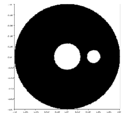
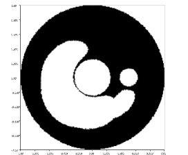
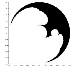
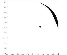
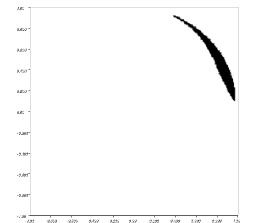
Figure 1: Example 1. The initial domain with cost $2.29164$ (top, left) and intermediary domains in the line search at the first iteration with cost $1.64609$ (top, middle), respectively $0.133162$ (top, right); the domains $\Omega_{n}$ for $n=1,3$ (bottom) using the descent direction (4.1).

As a second test, we use the descent direction

$$d_{n}=R\left(\frac{1}{\epsilon}w_{n}\right)$$ (4.2)

where $w_{n}$ is given by (4.1) and $R:\mathbb{R}\rightarrow\mathbb{R}$ is defined by

$$R(r)=\left\{\begin{array}[]{ll}-1+e^{r},&r<0,\\ 1-e^{-r},&r\geq 0.\end{array}\right.$$ (4.3)

The function $R$ is strictly increasing, $R\left(\mathbb{R}\right)=]-1,1[$, $R(-r)=-R(r)$ for all $r\in\mathbb{R}$.

Proposition 4.1

The direction $d_{n}$ defined by (4.2) where $w_{n}$ is given by (4.1) is a descent direction at $g_{n}$ for the cost function $j(g)=\frac{1}{2}\int_{\Omega}(y_{\epsilon}-y_{d})^{2}d\mathbf{x}$.

Proof. The directional derivative of the cost function was introduced in the previous section. In this particular case, the directional derivative of the cost function at $g_{n}$ in the direction $d_{n}$ is

$$\int_{D}\left(H^{\epsilon}\right)^{\prime}(g_{n})\left[\frac{1}{2}(y_{\epsilon}^{n}-y_{d})^{2}+\frac{1}{\epsilon}(y_{\epsilon}^{n}p^{n}+z_{\epsilon}^{n}q^{n})\right]d_{n}\,d\mathbf{x}.$$

It can be rewritten as

$$\int_{D}\left(H^{\epsilon}\right)^{\prime}(g_{n})(-w_{n})d_{n}\,d\mathbf{x} = \int_{D}\left(H^{\epsilon}\right)^{\prime}(g_{n})(-w_{n})R\left(\frac{1}{\epsilon}w_{n}\right)\,d\mathbf{x}$$

$$= -\epsilon\int_{D}\left(H^{\epsilon}\right)^{\prime}(g_{n})\left(\frac{1}{\epsilon}w_{n}\right)R\left(\frac{1}{\epsilon}w_{n}\right)\,d\mathbf{x}\leq 0.$$

For the last inequality, we have used that $\left(H^{\epsilon}\right)^{\prime}(g_{n})>0$ in $D$ and the property of the function $R$

$$rR(r)\geq 0,\quad\forall r\in\mathbb{R}$$

which gives $\left(\frac{1}{\epsilon}w_{n}\right)R\left(\frac{1}{\epsilon}w_{n}\right)\geq 0$ in $D$. Consequently, $d_{n}$ is a descent direction. We remark that this derivative is zero, if and only if $w_{n}=0$ in $D$. $\Box$

In this second test, excepting the descent direction, the other parameters are the same as before. The stopping test is obtained for $n=4$, the values of the cost function are: $j(g_{0})=2.29164$, $j(g_{1})=1.23291$, $j(g_{2})=0.295709$, $j(g_{3})=1.66212e-05$, $j(g_{4})=5.0583e-11$. The computed domains are presented in Figure 2. The optimal domain is the empty set and the optimal cost is zero, as obtained in both experiments.

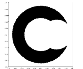
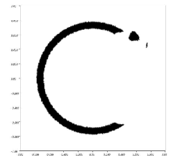
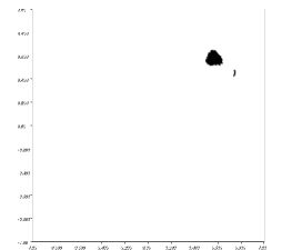
Figure 2: Example 1. The domains $\Omega_{n}$ for $n=0,1,2$ (top) and $n=3,4$ (bottom) using the descent direction (4.2).

Example 2.

We have again $D=]-1,1[\times]-1,1[$. The load is $f=1$, the cost function is $j(g)=\int_{\Omega}(y_{\epsilon}-y_{d})d\mathbf{x}$ where $y_{d}$ is given by

$$y_{d}(x_{1},x_{2})=\left\{\begin{array}[]{rl}1,&\hbox{if }\frac{1}{9}\leq x_{1}^{2}+x_{2}^{2}\leq\frac{1}{4}\\ -1,&\hbox{otherwise}.\end{array}\right.$$

We use for $D$ a mesh of 53360 triangles and 26981 vertices and for the approximation of $g$, $y$, $z$ we use piecewise linear finite element, globally continuous. The penalization parameter is $\epsilon=10^{-3}$.

The cost functional is of type (3.8) with $J\left(\mathbf{x},y_{\epsilon}(\mathbf{x})\right)=y_{\epsilon}-y_{d}$. From Corollary 3.1 and Remark 3.1, we get the following descent direction

$$w_{n}=-\left[(y_{\epsilon}^{n}-y_{d})+\frac{1}{\epsilon}(y_{\epsilon}^{n}p^{n}+z_{\epsilon}^{n}q^{n})\right].$$ (4.4)

The sequence $\left(j(g_{n})\right)_{n\in\mathbb{N}}$ is decreasing. For the stopping test, we use: if $j(g_{n+1})>j(g_{n})-tol$ then STOP, where $tol=10^{-6}$.

For the initial parametrization function $g_{0}(x_{1},x_{2})=-x_{1}^{2}-x_{2}^{2}+\frac{3}{4}$, that corresponds to a simply connected domain, the stopping test is obtained for $n=3$, the values of the cost function are: $j(g_{0})=1.51761$, $j(g_{1})=-0.417807$, $j(g_{2})=-0.421269$, $j(g_{3})=-0.423723$. Some computed domains are presented in Figure 3.

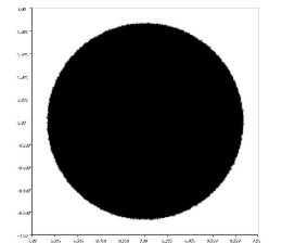
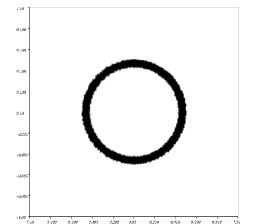
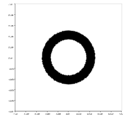
Figure 3: Example 2. The initial domain $\Omega_{0}$ with cost $1.51761$ (left), intermediary domain in the line search with cost $-0.203754$ (middle) and optimal domain $\Omega_{3}$ with cost $-0.423723$ (right), for initial parametrization $g_{0}(x_{1},x_{2})=-x_{1}^{2}-x_{2}^{2}+\frac{3}{4}$.

For the initial parametrization function used in Example 1, the stopping test is obtained for $n=6$, the values of the cost function are: $j(g_{0})=2.07908$, $j(g_{1})=-0.309447$, $j(g_{2})=-0.424$, $j(g_{3})=-0.424701$, $j(g_{4})=-0.425225$, $j(g_{5})=-0.425309$, $j(g_{6})=-0.425331$. Some computed domains are presented in Figure 4. The computed optimal cost depends slightly on $g_{0}$.

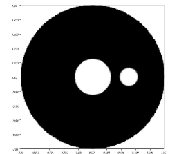
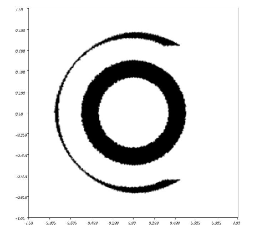
Figure 4: Example 2. The initial domain $\Omega_{0}$ with cost $2.07908$ (left), intermediary domains with cost $-0.309447$ (middle) and $-0.424$ (right), for initial parametrization $g_{0}$ used in Example 1.

Example 3.

We have again $D=]-1,1[\times]-1,1[$ and the cost function is $j(g)=\int_{\Omega}(y_{\epsilon}-y_{d})d\mathbf{x}$.

The load is $f=2\times 10^{3}$ and

$$y_{d}(x_{1},x_{2})=\left\{\begin{array}[]{rl}1,&\hbox{if }x_{1}^{2}+x_{2}^{2}\leq\frac{1}{4}\\ -1,&\hbox{otherwise}.\end{array}\right.$$

We use the direction

$$d_{n}=R\left(\frac{1}{\epsilon}w_{n}\right)$$ (4.5)

where $w_{n}$ is given by (4.4) and $R$ is defined by (4.3). As in Proposition 4.1, it yields that $d_{n}$ is a descent direction for the cost function $\int_{\Omega}(y_{\epsilon}-y_{d})d\mathbf{x}$. The other parameters are the same as in Example 1.

For the initial parametrization function $g_{0}(x_{1},x_{2})=-x_{1}^{2}-x_{2}^{2}+\frac{3}{4}$, used in Example 2, the stopping test is obtained for $n=5$, the values of the cost function are: $j(g_{0})=69.1791$, $j(g_{1})=15.5425$, $j(g_{2})=0.234407$, $j(g_{3})=-0.34875$, $j(g_{4})=-0.385096$, $j(g_{5})=-0.385548$. Some computed domains are presented in Figure 5.

For the initial parametrization function used in Example 1, the stopping test is reached for $n=3$ and the values of the cost function are: $j(g_{0})=20.2385$, $j(g_{1})=0.828123$, $j(g_{2})=-0.509888$, $j(g_{3})=-0.511685$. Some computed domains are presented in Figure 6. We observe that the obtained result depends on $g_{0}$. Shape optimization problems are strongly non convex and “local” solutions are obtained, in general.

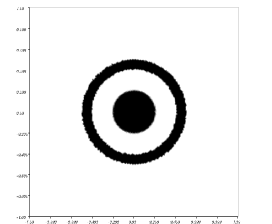
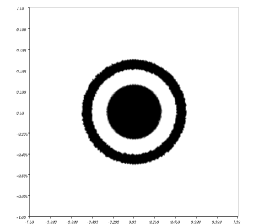
Figure 5: Example 3. The domains $\Omega_{n}$ for $n=0,3,5$ using the descent direction (4.5) and initial parametrization $g_{0}(x_{1},x_{2})=-x_{1}^{2}-x_{2}^{2}+\frac{3}{4}$.

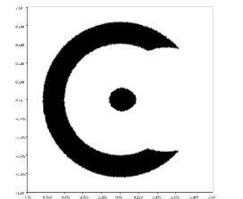
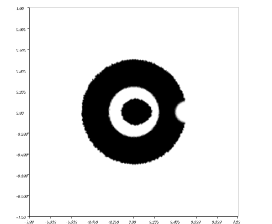
Figure 6: Example 3. The domains $\Omega_{n}$ for $n=0,1,3$ using the descent direction (4.5) for initial parametrization $g_{0}$ used in Example 1.

References

References

[1]
V. Arnautu, H. Langmach, J. Sprekels, D. Tiba,
On the approximation and the optimization of plates. Numer. Funct. Anal. Optim.
21 (2000),
no. 3-4, 337–354.
[2]
M. Barboteu, M. Sofonea, D. Tiba,
The control variational method for beams in contact with deformable obstacles,
Z. angew. Math. Mech., 92 (2012) no. 1, pp. 25–40.
[3]
D. Chenais,
On the existence of a solution in a domain identification
problem. J. Math. Anal. Appl. 52 (1975), no. 2, 189–219.
[4]
M.C. Delfour, J.P. Zolesio,
Shapes and Geometries, Analysis, Differential Calculus and Optimization,
SIAM, Philadelphia, 2001.
[5]
P. Grisvard,
Elliptic Problems in Nonsmooth Domains.
London, Pitman, 1985.
[6]
A. Halanay, C.M. Murea, D. Tiba,
Existence of a steady flow of Stokes fluid past a linear elastic structure
using fictitious domain,
J. Math. Fluid Mech. 18 (2016) 397–413.
[7] F. Hecht,
New development in FreeFem++.
J. Numer. Math. 20 (2012) 251–265.
http://www.freefem.org
[8]
B. Kawohl, J. Lang,
Are some optimal shape problems convex?
J. Convex Anal. 4 (1997), no. 2, 353–361.
[9]
J.-L. Lions,
Quelques méthodes de résolution des problèmes aux limites non linéaires,
Dunod, Paris,
1969.
[10]
R. Mäkinen, P. Neittaanmäki, D. Tiba,
On a fixed domain approach for a shape optimization problem.
In: W. F. Ames, P. J. van der Houwen (Eds), Computational and Applied
Mathematics II: Differential Equations, North-Holland, Amsterdam, 1992, pp. 317–326.
[11]
J. Muñoz, P. Pedregal,
A review of an optimal design problem for a plate of variable thickness.
SIAM J. Control Optim. 46 (2007), no. 1, 1–13.
[12]
C.M. Murea, D. Tiba,
A direct algorithm in some free boundary problems.
J. Numer. Math. 24 (2016) 253–271.
[13]
P. Neittaanmäki, A. Pennanen, D. Tiba,
Fixed domain approaches in shape optimization problems with Dirichlet
boundary conditions,
Inverse Problems 25 (2009) 1–18.
[14]
P. Neittaanmäki, J. Sprekels, D. Tiba,
Optimization of elliptic systems. Theory and applications, Springer,
New York, 2006.
[15]
P. Neittaanmäki, D. Tiba,
Fixed domain approaches in shape optimization problems,
Inverse Problems 28 (2012) 1–35.
[16]
O. Pironneau,
Optimal shape design for elliptic systems, Springer, Berlin, 1984.
[17]
P. Philip, D. Tiba,
Shape optimization via control of a shape function on a fixed domain:
theory and numerical results. In: S. Repin, T. Tiihonen, T. Tuovinen (Eds),
Numerical methods for differential equations, optimization and technological problems,
Computational methods in applied sciences 27, Springer Verlag, Dordrecht, 2013,
pp. 305–320.
[18]
M. Sofonea, D. Tiba,
The control variational method for contact of Euler-Bernoulli beams,
Bull. Transilvania Univ. Braşov vol. 2 (51), Series
III (2009), p.127–136.
[19]
J. Sokolowski, J.P. Zolesio,
Introduction to Shape Optimization. Shape Sensitivity Analysis,
Springer, Berlin,
1992.
[20]
J. Sprekels, D. Tiba,
Optimization of clamped plates with discontinuous thickness. Optimization and control
of distributed systems. Systems Control Lett. 48 (2003), no. 3-4, 289–295.
[21]
D. Tiba,
Domains of class C: properties and application.
Ann. of the Univ. of Bucharest (Ser. Math.), 4(LXII) (2013), 89–102.
[22]
D. Tiba,
Neumann boundary conditions in shape optimization,
Pure Appl. Funct. Anal.,
accepted (2017)