Random weighted averages, partition structures and generalized arcsine laws

Abstract

This article offers a simplified approach to the distribution theory of randomly weighted averages or $P$-means $M_{P}(X):=\sum_{j}X_{j}P_{j}$, for a sequence of i.i.d.random variables $X,X_{1},X_{2},\ldots$, and independent random weights $P:=(P_{j})$ with $P_{j}\geq 0$ and $\sum_{j}P_{j}=1$. The collection of distributions of $M_{P}(X)$, indexed by distributions of $X$, is shown to encode Kingman’s partition structure derived from $P$. For instance, if $X_{p}$ has Bernoulli$({p})$ distribution on $\{0,1\}$, the $n$th moment of $M_{P}(X_{p})$ is a polynomial function of ${p}$ which equals the probability generating function of the number $K_{n}$ of distinct values in a sample of size $n$ from $P$: ${\mathbb{E}}(M_{P}(X_{p}))^{n}={\mathbb{E}}{p}^{K_{n}}$. This elementary identity illustrates a general moment formula for $P$-means in terms of the partition structure associated with random samples from $P$, first developed by Diaconis and Kemperman (1996) and Kerov (1998) in terms of random permutations. As shown by Tsilevich (1997), if the partition probabilities factorize in a way characteristic of the generalized Ewens sampling formula with two parameters $(\alpha,\theta)$, found by Pitman (1995), then the moment formula yields the Cauchy-Stieltjes transform of an $(\alpha,\theta)$ mean. The analysis of these random means includes the characterization of $(0,\theta)$-means, known as Dirichlet means, due to Von Neumann (1941), Watson (1956), and Cifarelli and Regazzini (1990), and generalizations of Lévy’s arcsine law for the time spent positive by a Brownian motion, due to Darling (1949), Lamperti (1958), and Barlow, Pitman, and Yor (1989).

1 Introduction

Consider the randomly weighted average or $P$-mean of a sequence of random variables $(X_{1},X_{2},\ldots)$

$${\widetilde{X}}:=\sum_{j}X_{j}P_{j}$$ (1)

where $P:=(P_{1},P_{2},\ldots)$ is a random discrete distribution meaning that the $P_{j}$ are random variables with $P_{j}\geq 0$ and $\sum_{j}P_{j}=1$ almost surely, where $(X_{1},X_{2},\ldots)$ and $P$ are independent, and it is assumed that the series converges to a well defined limit almost surely. This article is concerned with characterizations of the exact distribution of ${\widetilde{X}}$ under various assumptions on the random discrete distribution $P$ and the sequence $(X_{1},X_{2},\ldots)$. Interest is focused on the case when the $X_{i}$ are i.i.d. copies of some basic random variable $X$. Then ${\widetilde{X}}$ is a well defined random variable, called the $P$-mean of $X$, whatever the distribution of $X$ with a finite mean, and whatever the random discrete distribution $P$ independent of the sequence of copies of $X$. These characterizations of the distribution of $P$-means are mostly known in some form. But the literature of random $P$-means is scattered, and the conceptual foundations of the theory have not been as well laid as they might have been. There has been recent interest in refined development of the distribution theory of $P$-means in various settings, especially for the model of distributions of $P$ indexed by two-parameters $(\alpha,\theta)$, whose size-biased presentation is known as GEM$(\alpha,\theta)$ after Griffiths, Engen and McCloskey, and whose associated partition probabilities were derived by Pitman (1995). See e.g. Regazzini et al. (2002), Regazzini et al. (2003), Lijoi and Regazzini (2004), James et al. (2008a), James (2010a, b), Lijoi and Prünster (2009). See also Ruggiero and Walker (2009), Petrov (2009), Canale et al. (2017), Lau (2013) for other recent applications of two-parameter model and closely related random discrete distributions, in which settings the theory of $(\alpha,\theta)$-means may be of further interest. So it may be timely to review the foundations of the theory of random $P$-means, with special attention to $P$ governed by the $(\alpha,\theta)$ model, and references to the historical literature and contemporary developments. The article is intended to be accessible even to readers unfamiliar with the theory of partition structures, and to provide motivation for further study of that theory and its applications to $P$-means.

The article is organized as follows. Section 2 offers an overview of the distribution theory of $P$-means, with pointers to the literature and following sections for details. Section 4 develops the foundations of a general distribution theory for $P$-means, essentially from scratch. Section 5 develops this theory further for some of the standard models of random discrete distributions. The aim is to explain, as simply as possible, some of the most remarkable known results involving $P$-means, and to clarify relations between these results and the theory of partition structures, introduced by Kingman (1975), then further developed in Pitman (1995), and surveyed in Pitman (2006, Chapters 2,3,4). The general treatment of $P$-means in Section 4 makes many connections to those sources, and motivates the study of partition structures as a tool for the analysis of $P$-means.

2 Overview

2.1 Scope

This article focuses attention on two particular instances of the general random average construction ${\widetilde{X}}:=\sum_{j}X_{j}P_{j}$.

• The $X_{j}$ are assumed to be independent and identically distributed (i.i.d.) copies of some basic random variable $X$, with the $X_{j}$ independent of $P$. Then ${\widetilde{X}}$ is called the $P$-mean of $X$, typically denoted $M_{P}(X)$ or ${\widetilde{X}}_{P}$.

• The case ${\widetilde{X}}:=X_{1}P_{1}+X_{2}\hbox{\vbox{\hrule height=0.5pt\kern 2.15277pt\hbox{\kern-1.00006pt$P$\kern-1.00006pt}}}_{1}$, with only two non-zero weights $P_{1}$ and $\hbox{\vbox{\hrule height=0.5pt\kern 2.15277pt\hbox{\kern-1.00006pt$P$\kern-1.00006pt}}}_{1}:=1-P_{1}$. It is assumed that $P_{1}$ is independent of $(X_{1},X_{2})$. But $X_{1}$ and $X_{2}$ might be independent and not identically distributed, or they might have some more general joint distribution.

Of course, more general random weighting schemes are possible, and have been studied to some extent. For instance, Durrett and Liggett (1983) treat the distribution of randomly weighted sums $\sum_{i}W_{i}X_{i}$ for random non-negative weights $W_{i}$ not subject to any constraint on their sum, and $(X_{i})$ a sequence of i.i.d. random variables independent of the weight sequence. But the theory of the two basic kinds of random averages indicated above is already very rich. This theory was developed in the first instance for real valued random variables $X_{j}$. But the theory extends easily to vector-valued random elements $X_{i}$, including random measures, as discussed in the next subsection.

Here, for a given distribution of $P$, the collection of distributions of $M_{P}(X)$, indexed by distributions of $X$, is regarded as an encoding of Kingman’s partition structure derived from $P$ (Corollary 9). That is, the collection of distributions of $\Pi_{n}$, the random partition of $n$ indices generated by a random sample of size $n$ from $P$. For instance, if $X_{p}$ has Bernoulli$(p)$ distribution on $\{0,1\}$, the $n$th moment of the $P$ mean of $X_{p}$ is a polynomial in $p$ of degree $n$, which is also the probability generating function of the number $K_{n}$ of distinct values in a sample of size $n$ from $P$: ${\mathbb{E}}(M_{P}(X_{p}))^{n}={\mathbb{E}}p^{K_{n}}$ (Proposition 10). This elementary identity illustrates a general moment formula for $P$-means, involving the exchangeable partition probability function (EPPF), which describes the distributions of $\Pi_{n}$ (Corollary 22). An equivalent moment formula, in terms of a random permutation whose cycles are the blocks of $\Pi_{n}$, was found by Diaconis and Kemperman (1996) for the $(0,\theta)$ model, and extended to general partition structures by Kerov (1998). As shown in Section 5.7, following Tsilevich (1997), this moment formula leads quickly to characterizations of the distribution of $P$-means when the EPPF factorizes in a way characteristic of the two-parameter family of GEM$(\alpha,\theta)$ models defined by a stick-breaking scheme generating $P$ from suitable independent beta factors. Then the moment formula yields the Cauchy-Stieltjes transform of an $(\alpha,\theta)$ mean ${\widetilde{X}}_{{\alpha,\theta}}$ derived from an i.i.d. sequence of copies of $X$. The analysis of these random $(\alpha,\theta)$ means ${\widetilde{X}}_{{\alpha,\theta}}$ includes the includes the characterization of $(0,\theta)$-means, commonly known as Dirichlet means, due to Von Neumann (1941), Watson (1956), and Cifarelli and Regazzini (1990), as well as generalizations of Lévy’s arcsine law for the time spent positive by a Brownian motion, due to Lamperti (1958), and Barlow, Pitman, and Yor (1989).

2.2 Random measures

To illustrate the idea of extending $P$-means from random variables to random measures, suppose that the $X_{j}$ are random point masses

$$X_{j}(\bullet):=\delta_{Y_{j}}(\bullet)=1(Y_{j}\in\bullet)$$

for a sequence of i.i.d. copies $Y_{j}$ of a random element $Y$ with values in an abstract measurable space $(S,\SS)$, with $\bullet$ ranging over $\SS$. Then

$$P(\bullet):=M_{P}(1(Y\in\bullet)):=\sum_{j}1(Y_{j}\in\bullet)P_{j}$$ (2)

is a measure-valued random $P$-mean. This is a discrete random probability measure on $(S,\SS)$ which places an atom of mass $P_{j}$ at location $Y_{j}$ for each $j$. Informally, $P(\bullet)$ is a reincarnation of $P=(P_{j})$ as a random discrete distribution on $(S,\SS)$ instead of the positive integers, obtained by randomly sprinkling the atoms $P_{j}$ over $S$ according to the distribution of $Y$. In particular, if the distribution of $Y$ is continuous, on the event of probability one that there are no ties between any two $Y$-values, the list of magnitudes of atoms of $P(\bullet)$ in non-increasing order is identical to the corresponding reordering $P^{\downarrow}$ of the sequence $P:=(P_{j},j=1,2,\ldots)$. The original random discrete distribution $P$ on positive integers, and the derived random discrete distribution $P(\bullet)$ on $(S,\SS)$, are then so similar, that using the same symbol $P$ for both of them seems justified. The integral of a suitable real-valued $\SS$-measurable function $g$ with respect to $P(\bullet)$ is just the $P$-mean of the real-valued random variable $g(Y)$:

$$\int_{S}g(s)P(ds)=M_{P}(g(Y)):=\sum_{j}g(Y_{j})P_{j}.$$ (3)

Hence the analysis of random probability measures $P(\bullet)$ of the form (2) on an abstract space $(S,\SS)$ reduces to an analysis of distributions of $P$-means $M_{P}(X)$ for real-valued $X=g(Y)$. For $P$ a listing of the normalized jumps of a standard gamma process $(\gamma(r),0\leq r\leq\theta)$, that is a subordinator, or increasing process with stationary independent increments, with

$${\mathbb{P}}(\gamma(r)\in dx)/dx=\frac{1}{\Gamma(r)}x^{r-1}e^{-x}1(x>0),$$ (4)

formula (2) is Ferguson’s (1973) construction of a Dirichlet random probability measure $P(\bullet)$ on $(S,\SS)$ governed by the measure $\theta\,{\mathbb{P}}(Y\in\bullet)$ with total mass $\theta$. For $r,s>0$ let $\beta_{r,s}$ denote a random variable with the beta$(r,s)$ distribution on $[0,1]$

$${\mathbb{P}}(\beta_{r,s}\in du)/du=\frac{\Gamma(r+s)}{\Gamma(r)\Gamma(s)}\,u^{r-1}(1-u)^{s-1}1(0<u<1).$$ (5)

Such a beta $(r,s)$ variable is conveniently constructed from the standard gamma process $(\gamma(r),r\geq 0)$ by the beta-gamma algebra

$$\beta_{r,s}:=\frac{\gamma(r)}{\gamma(r+s)}=\frac{\gamma(r)}{\gamma(r)+\gamma^{\prime}(s)}$$ (6)

where $\gamma^{\prime}(s):=\gamma(r+s)-\gamma(r)\stackrel{{\scriptstyle d}}{{=}}\gamma(s)$ is a copy of $\gamma(s)$ that is independent of $\gamma(r)$, and

$$\beta_{r,s}\mbox{ and }\gamma(r+s)\mbox{ are independent.}$$ (7)

As a consequence, for $g(s)=1(s\in B)$ in (3), so $g(X)$ has the Bernoulli$(p)$ distribution on $\{0,1\}$ for $p={\mathbb{P}}(Y\in B)$, the simplest Dirichlet mean (3) for an indicator variable has a beta distribution:

$$P(B)\stackrel{{\scriptstyle d}}{{=}}\beta_{p\theta,q\theta}\mbox{ for }p:={\mathbb{P}}(Y\in B),\qquad q:=1-p.$$ (8)

See Section 5.3 for further disussion.

Replacing the gamma process by a more general subordinator makes $P(\bullet)$ a homogeneous normalized random measure with independent increments (HRMI) as studied by Regazzini et al. (2003), James et al. (2009). from the perspective of Bayesian inference for $P(\bullet)$ given a random sample of size $n$ from $P(\bullet)$. Basic properties of $P$-means derived from normalized subordinators are developed here in Section 5.2.

2.3 Splitting off the first term

It is a key observation that the $P$-mean of an i.i.d. sequence can sometimes be expressed as a $(P_{1},\hbox{\vbox{\hrule height=0.5pt\kern 2.15277pt\hbox{\kern-1.00006pt$P$\kern-1.00006pt}}}_{1})$-mean by the splitting off the first term. That is the decomposition

$${\widetilde{X}}_{P} :=\sum_{j=1}^{\infty}X_{j}P_{j}$$ (9)

$$=X_{1}P_{1}+{\widetilde{X}}_{R}\,\hbox{\vbox{\hrule height=0.5pt\kern 2.15277pt\hbox{\kern-1.00006pt$P$\kern-1.00006pt}}}_{1}\mbox{ where }{\widetilde{X}}_{R}:=\sum_{j=1}^{\infty}X_{j+1}R_{j}$$ (10)

with $R_{j}:=P_{j+1}/\hbox{\vbox{\hrule height=0.5pt\kern 2.15277pt\hbox{\kern-1.00006pt$P$\kern-1.00006pt}}}_{1}$ the residual probability sequence defined on the event $\hbox{\vbox{\hrule height=0.5pt\kern 2.15277pt\hbox{\kern-1.00006pt$P$\kern-1.00006pt}}}_{1}>0$ by first conditioning $P$ on $\{2,3,\ldots\}$ and then shifting back to $\{1,2,\ldots\}$. In general, the residual sequence $R$ may be dependent on $P_{1}$. Then ${\widetilde{X}}_{R}$ and $P_{1}$ will typically not be independent, and analysis of ${\widetilde{X}}_{P}$ will be difficult. However,

if $$P_{1} (R_{1},R_{2},\ldots)$$ and are independent, (11)

then $P_{1}$, $X_{1}$ and ${\widetilde{X}}_{R}$ are mutually independent. So

$${\widetilde{X}}_{P}=X_{1}P_{1}+{\widetilde{X}}_{R}\hbox{\vbox{\hrule height=0.5pt\kern 2.15277pt\hbox{\kern-1.00006pt$P$\kern-1.00006pt}}}_{1}.$$ (12)

The right side is the $(P_{1},\hbox{\vbox{\hrule height=0.5pt\kern 2.15277pt\hbox{\kern-1.00006pt$P$\kern-1.00006pt}}}_{1})$-mean of $X_{1}$ and ${\widetilde{X}}_{R}$, with $P_{1}$ independent of $X_{1}$ and ${\widetilde{X}}_{R}$, which are independent but typically not identically distributed.

This basic decomposition of a $P$-mean by splitting off the first term leads naturally to discussion of $P$-means for random discrete distributions defined by a recursive splitting of this kind, called residual allocation models or stick-breaking schemes, discussed further in Section 5.1.

2.4 Lévy’s arcsine laws

An inspirational example of splitting off the first term is provided by the work of Lévy (1939) on the distributions of the time $A_{t}$ spent positive up to time $t$, and the time $G_{t}$ of the last zero before time $t$, for a standard Brownian motion $B$:

$$A_{t}:=\int_{0}^{t}1(B_{u}>0)du\qquad\mbox{and}\qquad G_{t}:=\max\{0\leq u\leq t:B_{u}=0\},$$

See e.g. Kallenberg (2002, Theorem 13.16) for background. To place this example in the framework of $P$-means:

• Let $P_{1}:=1-G_{1}$ be the length of the meander interval $(G_{1},1)$.

• Let $X_{1}:=1(B_{1}>0)$ be the indicator of the event $(B_{1}>0)$ with Bernoulli $(\mbox{$\frac{1}{2}$})$ distribution.

• Let $(P_{j},X_{j})$ for $j\geq 2$ be an exhaustive listing of the lengths $P_{j}$ of excursion intervals of $B$ away from $0$ on $(0,G_{1})$, with $X_{j}$ the indicator of the event that $B_{t}>0$ for $t$ in the excursion interval of length $P_{j}$.

If the lengths $P_{j}$ for $j\geq 2$ are put in a suitable order, for instance by ranking, then $(X_{j},j\geq 1)$ will be a sequence of i.i.d. copies of a Bernoulli $(\mbox{$\frac{1}{2}$})$ variable $X_{\mbox{$\frac{1}{2}$}}$, with $(X_{j},j\geq 1)$ independent of the excursion lengths $(P_{j},j\geq 1)$. Then by construction,

$$A_{1}=M_{P}(X_{\mbox{$\frac{1}{2}$}})$$

is the $P$-mean of a Bernoulli $(\mbox{$\frac{1}{2}$})$ indicator $X_{\mbox{$\frac{1}{2}$}}$, representing the sign of a generic excursion. This is so for any listing $P$ of excursion lengths of $B$ on $[0,1]$ that is independent of their signs. But if $P_{1}:=1-G_{1}$ puts the meander length first as above, then the residual sequence $(R_{1},R_{2},\ldots)$ is identified with the sequence of relative lengths of excursions away from zero of $B$ on $[0,G_{1}]$. But that is also the list of excursion lengths of the rescaled process ${B^{\rm br}}:=(B(uG_{1})/\sqrt{G_{1}},0\leq u\leq 1)$, with corresponding positivity indicators $(X_{2},X_{3},\ldots)$. Lévy showed that ${B^{\rm br}}$ is a standard Brownian bridge, equivalent in distribution to $(B_{u},0\leq u\leq 1\,|\,B_{1}=0)$, and that a last exit decomposition of the path of $B$ at time $G_{1}$ makes the length $P_{1}$ of the meander interval independent of ${B^{\rm br}}$, hence also independent of the residual sequence $(R_{1},R_{2},\ldots)$ and the positivity indicators $(X_{2},X_{3},\ldots)$, which are encoded in the path of ${B^{\rm br}}$. Let $A^{\rm br}_{1}$ denote the total time spent positive by this Brownian bridge ${B^{\rm br}}$. So $A^{\rm br}_{1}\stackrel{{\scriptstyle d}}{{=}}(A_{1}|B_{1}=0)$, while also $A^{\rm br}_{1}=\sum_{j=1}^{\infty}R_{j}X_{j+1}$ by the previous construction. Then the last exit decomposition provides a splitting of $A_{1}=M_{P}(X)$ of the general form (12). In this instance,

$$A_{1}=X_{1}P_{1}+A^{\rm br}_{1}\,\hbox{\vbox{\hrule height=0.5pt\kern 2.15277pt\hbox{\kern-1.00006pt$P$\kern-1.00006pt}}}_{1}$$ (13)

where on the right side

• $X_{1},P_{1}$ and $A^{\rm br}_{1}$ are independent, with

• $X_{1}=1(B_{1}>0)\stackrel{{\scriptstyle d}}{{=}}X_{\mbox{$\frac{1}{2}$}}$ a Bernoulli$(\mbox{$\frac{1}{2}$})$ indicator,

• $P_{1}$ the meander length,

• $A^{\rm br}_{1}$ the total time spent positive by ${B^{\rm br}}$, and

• $\hbox{\vbox{\hrule height=0.5pt\kern 2.15277pt\hbox{\kern-1.00006pt$P$\kern-1.00006pt}}}_{1}:=1-P_{1}=G_{1}$ the last exit time.

Lévy showed the meander interval has length $P_{1}\stackrel{{\scriptstyle d}}{{=}}\beta_{\mbox{$\frac{1}{2}$},\mbox{$\frac{1}{2}$}}$, known as the arcsine law, because

$${\mathbb{P}}(\beta_{\mbox{$\frac{1}{2}$},\mbox{$\frac{1}{2}$}}\leq u)=\frac{2}{\pi}\arcsin\sqrt{u}\qquad(0\leq u\leq 1),$$ (14)

while the bridge occupation time has the uniform $[0,1]$ distribution $A^{\rm br}_{1}\stackrel{{\scriptstyle d}}{{=}}\beta_{1,1}$. Lévy then deduced from (13) that the unconditioned occupation time $A_{1}$ has the same arcsine distribution as $P_{1}$ and $G_{1}=\hbox{\vbox{\hrule height=0.5pt\kern 2.15277pt\hbox{\kern-1.00006pt$P$\kern-1.00006pt}}}_{1}$:

$$A_{1}\stackrel{{\scriptstyle d}}{{=}}P_{1}\stackrel{{\scriptstyle d}}{{=}}G_{1}\stackrel{{\scriptstyle d}}{{=}}\beta_{\mbox{$\frac{1}{2}$},\mbox{$\frac{1}{2}$}}.$$ (15)

2.5 Generalized arcsine laws

Lévy’s arcsine laws (15) for the Brownian occupation time $A_{1}$, the time $G_{1}$ of the last zero in $[0,1]$, and the meander length $P_{1}:=1-G_{1}$, and his associated uniform law for the Brownian bridge occupation times $A^{\rm br}_{1}$, have been generalized in several different ways. One of the most far-reaching of these generalizations gives corresponding results when the basic Brownian motion $B$ is replaced by process with exchangeable increments. Discrete time versions of these results were first developed by Andersen (1953). Feller (1971, §XII.8 Theorem 2) gave a refined treatment, with the following formulation for a random walk $S_{n}:=X_{1}+\cdots+X_{n}$ with exchangeable increments $(X_{i})$, started at $S_{0}:=0$: the random number of times $\sum_{i=1}^{n}1(S_{i}>0)$ that the walk is strictly positive up to time $n$ has the same distribution as the random index $\min\{0\leq k\leq n:S_{k}=M_{n}\}$ at which the walk first attains its maximum value $M_{n}:=\max_{0\leq k\leq n}S_{k}$. In the Brownian scaling limit, Sparre Andersen’s identity implies the equality in distribution $A_{1}\stackrel{{\scriptstyle d}}{{=}}G^{\rm max}_{1}$, the last time in $[0,1]$ that Brownian motion attains its maximum on $[0,1]$. That the distribution of $G^{\rm max}_{1}$ is arcsine was shown also by Lévy, who then argued that $G^{\rm max}_{1}\stackrel{{\scriptstyle d}}{{=}}G_{1}$, the time of the last zero of $B$ on $[0,1]$, by virtue of his famous identity in distribution of reflecting processes

$$(M_{t}-B_{t},t\geq 0)\stackrel{{\scriptstyle d}}{{=}}(|B_{t}|,t\geq 0)$$ (16)

where $M_{t}:=\max_{0\leq s\leq t}B_{s}$ is the running maximum process derived from the path of $B$.

Many other generalizations of the arcsine law have been developed, typically starting from one of the many ways this distribution arises from Brownian motion, or from one of its many characterizations by identities in distribution or moment evaluations. See for instance Kallenberg (2002, Theorem 15.21) for the result that Lévy’s arcsine law (15) extends to the occupation time $A_{1}$ of $(0,\infty)$ up to time $1$ for any symmetric Lévy process $X$ with ${\mathbb{P}}(X_{t}=0)=0$ instead of $B$, with $G_{1}$ replaced by $G^{\rm max}_{1}$, the last time in $[0,1]$ that $X$ attains its maximum on $[0,1]$, and $P_{1}$ replaced by $1-G^{\rm max}_{1}$. See also Takács (1996a, b, 1999, 1998), Petit (1992) and Mansuy and Yor (2008, Chapter 8) regarding the distribution of occupation times of Brownian motion with drift and other processes derived from Brownian motion. See Getoor and Sharpe (1994), Bertoin and Yor (1996), Bertoin and Doney (1997) for more general results on Lévy processes, and Knight (1996) and Fitzsimmons and Getoor (1995), for an extension of the uniform distribution of $A^{\rm br}_{1}$ for Brownian motion to more general bridges with exchangeable increments, and Yano (2006) for an extension to conditioned diffusions. Watanabe (1995) gave generalized arc-sine laws for occupation times of half lines of one-dimensional diffusion processes and random walks, which were further developed in Kasahara and Yano (2005) and Watanabe et al. (2005). Yet another generalization of the arcsine law was proposed by Lijoi and Nipoti (2012).

The focus here is on generalized arcsine laws involving the distributions of $P$-means for some random discrete distribution $P$. The framing of Lévy’s description of the laws of the Brownian occupation times $A_{1}$ and $A^{\rm br}_{1}$, as $P$-means of a Bernoulli$(\mbox{$\frac{1}{2}$})$ variable, for distributions of $P$ determined by the lengths of excursions of a Brownian motion or Brownian bridge, inspired the work of Barlow, Pitman, and Yor (1989) and Pitman and Yor (1992). These articles showed how Lévy’s analysis could be extended by consideration of the path of $(B_{t},0\leq t\leq T)$ for a random time $T$ independent of $B$ with the standard exponential distribution of $\gamma(1)$. For then $G_{T}/T\stackrel{{\scriptstyle d}}{{=}}G_{1}$ by Brownian scaling, while the last exit decomposition at time $G_{T}$ breaks the path of $B$ on $[0,T]$ into two independent random fragments of random lengths $G_{T}$ and $T-G_{T}$ respectively. Thus

$$G_{1}\stackrel{{\scriptstyle d}}{{=}}\frac{G_{T}}{T}=\frac{G_{T}}{G_{T}+(T-G_{T})}\stackrel{{\scriptstyle d}}{{=}}\frac{\gamma(\mbox{$\frac{1}{2}$})}{\gamma(\mbox{$\frac{1}{2}$})+\gamma^{\prime}(\mbox{$\frac{1}{2}$})}\stackrel{{\scriptstyle d}}{{=}}\beta_{\mbox{$\frac{1}{2}$},\mbox{$\frac{1}{2}$}}.$$

This realizes the instance $r=s=\mbox{$\frac{1}{2}$}$ of the beta-gamma algebra (6) in the path of Brownian motion stopped at the independent gamma$(1)$ distributed random time $T$. A similar subordination construction was exploited earlier by Greenwood and Pitman (1980) in their study of fluctuation theory for Lévy processes by splitting at the time $G^{\rm max}_{T}$ of the last maximum before an independent exponential time $T$. See Bertoin (1996) and Kyprianou (2014) for more recent accounts of this theory. This involves the lengths of excursions of the Lévy process below its running maximum process $M$. Lévy recognized that for a Brownian motion $B$ his famous identity in law of processes $M-B\stackrel{{\scriptstyle d}}{{=}}|B|$, as in (16), implied that the structure of excursions of $B$ below $M$ is identical to the structure of excursions of $|B|$ away from $0$. This leads from the decomposition of $M-B$ at the time $G^{\rm max}_{T}$ of the last zero of $M-B$ on $[0,T]$ to the corresponding decomposition for $|B|$, discussed earlier. The same method of subordination was exploited further in Pitman and Yor (1997a, Proposition 21), in a deeper study of random discrete distributions derived from stable subordinators.

The above analysis of the $P$-mean $M_{P}(X)$, for an indicator variable $X=X_{\mbox{$\frac{1}{2}$}}$, and $P$ the list of lengths of excursions of a Brownian motion or Brownian bridge, was generalized by Barlow, Pitman, and Yor (1989) to allow any discrete distribution of $X$ with a finite number of values. That corresponds to a linear combination of occupation times of various sectors in the plane by Walsh’s Brownian motion on a finite number of rays, whose radial part is $|B|$, and whose angular part is made by assigning each excursion of $|B|$ to the $i$th ray with some probability $p_{i}$, independently for different excursions. The analysis up to an independent exponential time $T$ relies only on the scaling properties of $|B|$, the Poisson character of excursions of $|B|$, and beta-gamma algebra, all of which extend straightforwardly to the case when $|B|$ is replaced by a Bessel process or Bessel bridge of dimension $2-2\alpha$, for $0<\alpha<1$. Then $P$ becomes a list of excursion lengths of the Bessel process or bridge over $[0,1]$, while $G_{T}$ and $T-G_{T}$ become independent gamma$(\alpha)$ and gamma$(1-\alpha)$ variables with sum $T$ that is gamma$(1)$. So the distribution of the final meander length in the stable $(\alpha)$ case is given by

$$P_{1}\stackrel{{\scriptstyle d}}{{=}}\frac{T-G_{T}}{T}\stackrel{{\scriptstyle d}}{{=}}\beta_{1-\alpha,\alpha}$$ (17)

by another application of the beta-gamma algebra (6). The excursion lengths $P$ in this case are a list of lengths of intervals of the relative complement in $[0,1]$ of the range of a stable subordinator of index $\alpha$, with conditioning of this range to contain $1$ in the bridge case. In particular, for $0<p<1$, the $P$-mean of a Bernoulli$(p)$ indicator $X_{p}$ represents the occupation time of the positive half line for a skew Brownian motion or Bessel process, each excursion of which is positive with probability $p$ and negative with probability $1-p$. The distribution of such a $P$-mean, say $M_{\alpha,0}(X_{p})$, associated with a stable subordinator of index $\alpha\in(0,1)$ and a selection probability parameter $p\in(0,1)$, was found independently by Darling (1949) and Lamperti (1958). Darling indicated the representation

$$M_{\alpha,0}(X_{p})\stackrel{{\scriptstyle d}}{{=}}T_{\alpha}(p)/T_{\alpha}(1)$$

where $(T_{\alpha}(s),s\geq 0)$ is the stable subordinator with

$${\mathbb{E}}\exp(-\lambda T_{\alpha}(s))=\exp(-s\lambda^{\alpha})\qquad(\lambda\geq 0).$$ (18)

Darling also presented a formula for the cumulative distribution function of $M_{\alpha,0}(X_{p})$, corresponding to the probability density

$$\frac{{\mathbb{P}}(M_{\alpha,0}(X_{p})\in du)}{du}=\frac{pq\sin(\alpha\pi)u^{\alpha-1}\hbox{\vbox{\hrule height=0.5pt\kern 2.15277pt\hbox{\kern-1.00006pt$u$\kern-1.00006pt}}}^{\alpha-1}}{\pi[q^{2}u^{2\alpha}+2pqu^{\alpha}\hbox{\vbox{\hrule height=0.5pt\kern 2.15277pt\hbox{\kern-1.00006pt$u$\kern-1.00006pt}}}^{\alpha}\cos(\alpha\pi)+p^{2}\hbox{\vbox{\hrule height=0.5pt\kern 2.15277pt\hbox{\kern-1.00006pt$u$\kern-1.00006pt}}}^{2\alpha}]}\qquad(0<u<1)$$ (19)

where $q:=1-p$ and $\hbox{\vbox{\hrule height=0.5pt\kern 2.15277pt\hbox{\kern-1.00006pt$u$\kern-1.00006pt}}}:=1-u$. Later, Zolotarev (1957) derived the corresponding formula for the density of the ratio of two independent stable$(\alpha)$ variables $T_{\alpha}(p)/(T_{\alpha}(1)-T_{\alpha}(p))$ by Mellin transform inversion. This makes a surprising connection between the stable$(\alpha)$ subordinator and the Cauchy distribution, discussed further in Section 3. Lamperti (1958) showed that the density of $M_{\alpha,0}(X_{p})$ displayed in (19) is the density of the limiting distribution of occupation times of a recurrent Markov chain, under assumptions implying that the return time of some state is in the domain of attraction of the stable law of index $\alpha$, and between visits to this state the chain enters some given subset of its state space with probability $p$. Lamperti’s approach was to first derive the the Stieltjes transform

$${\mathbb{E}}(1+\lambda M_{\alpha,0}(X_{p}))^{-1}=\sum_{n=0}^{\infty}{\mathbb{E}}(M_{\alpha,0}(X_{p}))^{n}\lambda^{n}=\frac{q+p(1+\lambda)^{\alpha-1}}{q+p(1+\lambda)^{\alpha}}$$ (20)

where $q:=1-p$. The associated beta$(1-\alpha,\alpha)$ distribution of $P_{1}$ appearing in (17) is also known as a generalized arcsine law. In Lamperti’s setting of a chain returning to a recurrent state, the results of Dynkin (1961), presented also in Feller (1971, §XIV.3), imply that Lamperti’s limit law for occupation times holds jointly with convergence in distribution of the fraction of time since last visit to the recurrent state to the meander length $P_{1}$ as in (17), along with the generalization to this case of the distributional identity (13), which was exploited by Barlow, Pitman, and Yor (1989). Due to the results of Sparre Andersen mentioned earlier, this beta$(1-\alpha,\alpha)$ distribution also arises from random walks and Lévy processes as both a limit distribution of scaled occupation times, and as the exact distribution of the occupation time of the positive half line for a limiting stable Lévy process $X_{t}$ with ${\mathbb{P}}(X_{t}>0)=1-\alpha$ for all $t$. But in the context of the $(\alpha,0)$ model for $P$, this beta$(1-\alpha,\alpha)$ distribution appears either as the distribution of the length of the meander interval $P_{1}$, as in (17), or as the distribution of a size-biased pick $P_{1}^{*}$ from $P$. See also Pitman and Yor (1992) and (Pitman and Yor, 1997b, §4) for closely related results, and James (2010b) for an authoritative recent account of further developments of Lamperti’s work.

2.6 Fisher’s model for species sampling

A parallel but independent development of closely related ideas, from the 1940’s to the 1990’s, was initiated by Fisher (1943). See Pitman (1996b) for a review. Fisher introduced a theoretical model for species sampling, which amounts to random sampling from the random discrete distribution $(P_{1},\ldots,P_{m})$ with the symmetric Dirichlet distribution with $m$ parameters equal to $\theta/m$ on the $m$-simplex of $(P_{1},\ldots,P_{m})$ with $P-i\geq 0$ and $\sum_{i=1}^{m}P_{i}=1$. See Section 5.3 for a quick review of basic properties of Dirichlet distributions. Fisher showed that many features of sampling from this symmetric Dirichlet model for $P$ have simple limit distributions as $m\to\infty$ with $\theta$ fixed. Ignoring the order of the $P_{i}$, the limit model may be constructed directly by supposing that the $P_{i}$ are the normalized jumps of a standard gamma process on the interval $[0,\theta]$. That model for a random discrete distribution, called here the $(0,\theta)$ model, was considered by McCloskey (1965) as an instance of the more general model, discussed in Section 5.2 in which the $P_{i}$ are the normalized jumps of a subordinator on a fixed time interval $[0,\theta]$, which for a stable $(\alpha)$ subordinator corresponds to the $(\alpha,0)$ model involved in the Lévy-Lamperti description of occupation times. McCloskey showed that if the atoms of $P$ in the $(0,\theta)$ model are presented in the size-biased order $P^{*}$ of their appearance in a process of random sampling, then $P^{*}$ admits a simple stick-breaking representation by a recursive splitting like (9) with i.i.d. factors $P^{*}_{j}/(1-P^{*}_{1}-\cdots-P^{*}_{j-1})\stackrel{{\scriptstyle d}}{{=}}\beta_{1,\theta}$. Engen (1975) interpreted this GEM$(0,\theta)$ model as the limit in distribution of size-biased frequencies in Fisher’s limit model. This presentation of $(0,\theta)$ model was developed in various ways by Patil and Taillie (1977), Sethuraman (1994), and Pitman (1996a). In this model for $P=P^{*}$ in size-biased random order, the basic splitting (12) holds with a residual sequence $R$ that is identical in law to the original sequence $P$, hence also ${\widetilde{X}}_{R}\stackrel{{\scriptstyle d}}{{=}}{\widetilde{X}}_{P}$. Then (12) becomes a characterization of the law of ${\widetilde{X}}_{P}$ by a stochastic equation which typically has a unique solution, as discussed in Feigin and Tweedie (1989), Diaconis and Freedman (1999), Hjort and Ongaro (2005). See also Bacallado et al. (2017) for a recent review of species sampling models.

Ferguson (1973) and Kingman (1975) further developed McCloskey’s model of $P$ derived from the normalized jumps of subordinator, working instead with the ranked rearrangement $P^{\downarrow}$ of $P$ with $P^{\downarrow}_{1}\geq P^{\downarrow}_{2}\geq\cdots\geq 0$. However, it is easily seen that the distribution of the $P$-mean of a sequence of i.i.d. copies of $X$ is unaffected by any reordering of terms of $P$, provided the reordering is made independently of the copies of $X$. So for any random discrete distribution $P$, and any distribution of $X$, there is the equality in distribution

$$M_{P}(X)\stackrel{{\scriptstyle d}}{{=}}M_{P}^{\downarrow}(X)\stackrel{{\scriptstyle d}}{{=}}M_{P^{*}}(X)$$ (21)

where $P^{*}$ can be any random rearrangement of terms of $P$. This invariance in distribution of $P$-means under re-ordering of the atoms of $P$ is fundamental to understanding the general theory of $P$-means. In the analysis of $M_{P}(X)$ by splitting off the first term, the distribution of $M_{P}(X)$ is the same, no matter how the terms of $P$ may be ordered. But the ease of analysis depends on the joint distribution of $P_{1}$ and $(P_{2},P_{3},\ldots)$, which in turn depends critically on the ordering of terms of $P$. Detailed study of problems of this kind by Pitman (1996a) explained why the size-biased random permutation of terms $P^{*}$, first introduced by McCloskey in the setting of species sampling, is typically more tractable than the ranked ordering used by Ferguson and Kingman. The notation $P^{*}$ will be used consistently below to indicate a size-biased ordering of terms in a random discrete distribution.

2.7 The two-parameter family

The articles of Perman et al. (1992) and Pitman and Yor (1997a). introduced a family of random discrete distributions indexed by two-parameters $(\alpha,\theta)$, which includes the various examples recalled above in a unified way. Various terminology is used for different encodings of this family of random discrete distributions and associated random partitions.

• The distribution of the size-biased random permutation $P^{*}$ is known as GEM$(\alpha,\theta)$, after Griffiths, Engen and McCloskey, who were among the first to study the simple stick-breaking description of this model recalled later in (150).

• The distribution of the corresponding ranked arrangement $P^{\downarrow}$ is known as the two-parameter Poisson-Dirichlet distribution (Pitman and Yor, 1997a), (Feng, 2010).

• The corresponding random discrete probability measure on an abstract space $(S,\SS)$, constructed as in (2) by assigning the GEM or Poisson-Dirichlet atoms i.i.d. locations in $S$, has become known as a Pitman-Yor process. (Ishwaran and James, 2001).

• The corresponding partition structure is governed by the sampling formula of Pitman (1995) which is a two parameter generalization of the Ewens sampling formula, recently reviewed by Crane (2016).

• The $P$-means associated with the $(0,\theta)$ model are commonly called Dirichlet means (James et al., 2008b), (James, 2010a).

The $(\alpha,\theta)$ model refers here to this model of a random discrete distribution $P$, whose size-biased presentation is GEM$(\alpha,\theta)$. For such a $P$ the associated $P$-mean will be called simply an $(\alpha,\theta)$-mean, with similar terminology for other attributes of the $(\alpha,\theta)$ model, such as its partition structure.

Following further work by numerous authors including Cifarelli and Regazzini (1990), Diaconis and Kemperman (1996) and Kerov (1998), a definitive formula characterizing the distribution of an $(\alpha,\theta)$ mean ${\widetilde{X}}_{{\alpha,\theta}}$, for an arbitary distribution of a bounded or non-negative random variable $X$, was found by Tsilevich (1997): for all $(\alpha,\theta)$ for which the model is well defined, except if $\alpha=0$ or $\theta=0$, the distribution of ${\widetilde{X}}_{{\alpha,\theta}}$ is uniquely determined by the generalized Cauchy-Stieltjes transform

$${\mathbb{E}}(1+\lambda{\widetilde{X}}_{\alpha,\theta})^{-\theta}=\left({\mathbb{E}}(1+\lambda X)^{\alpha}\right)^{-{\frac{\theta}{\alpha}}}\qquad(\alpha\neq 0,\theta\neq 0,\lambda\geq 0).$$ (22)

Companion formulas for the $(\alpha,0)$ case with $\theta=0$, $0<\alpha<1$, trace back to Lamperti for $X=X_{p}$ a Bernoulli$(p)$ variable, as in (20), while the $(0,\theta)$ case with $\alpha=0,\theta>0$ is the case of Dirichlet means due to Von Neumann (1941), and Watson (1956) in the classical setting of mathematical statistics, involving ratios of quadratic forms of normal variables, and developed by Cifarelli and Regazzini (1990) and others in Ferguson’s Bayesian non-parametric setting. These formulas are all obtained as limit cases of the generic two-parameter formula (22), naturally involving exponentials and logarithms due to the basic approximations of these functions by large or small powers as the case may be e.g. $e^{x}=\lim_{n\to\infty}(1+x/n)^{n}$ and $\log x=\lim_{\alpha\downarrow 0}(x^{\alpha}-1)/\alpha$ for $x>0$. For $\theta=\alpha\in(0,1)$ the transform (22) was obtained earlier by Barlow et al. (1989) in their description of the distribution of occupation times derived from a Brownian or Bessel bridge, by a straightforward argument from the perspective of Markovian excursion theory. But Tsilevich’s extension of this formula to general $(\alpha,\theta)$ is not obvious from that perspective. Rather, the simplest approach to Tsilevich’s formula involves analysis of partition structure associated with $(\alpha,\theta)$ model, as discussed in Section 5.7.

Further development of the theory of $(\alpha,\theta)$ means was made by Vershik, Yor, and Tsilevich (2001). See also the articles by James, Lijoi and coauthors, listed in the introduction, for the most refined analysis of $(\alpha,\theta)$-means by inversion of the Cauchy-Stieltjes transform.

3 Transforms

Typical arguments for identifying the distribution of a $P$-mean involve encoding the distribution by some kind of transform. This section reviews some probabilistic techniques for handling such transforms, by study of some key examples related to ratios of independent stable variables. See Chaumont and Yor (2003) for further exercises with these techniques, and James (2010b) for many deeper results in this vein.

3.1 The Talacko-Zolotarev distribution

The following proposition was discovered independently in different contexts by Talacko (1956) and Zolotarev (1957, Theorem 3).

Proposition 1.

[Talacko-Zolotarev distribution]. Let $C$ denote a standard Cauchy variable with probability density ${\mathbb{P}}(C\in dc)=\pi^{-1}(1+c^{2})^{-1}dc$ for $c\in{\mathbb{R}}$, and

$$C_{\alpha}:=-\cos({\alpha\pi})+\sin({\alpha\pi})\,C\qquad(0\leq\alpha\leq 1).$$ (23)

Let $S_{\alpha}$ be a random variable with the conditional distribution of $\log C_{\alpha}$ given the event $(C_{\alpha}>0)$, with $P(C_{\alpha}>0)=\alpha$:

$$S_{\alpha}\stackrel{{\scriptstyle d}}{{=}}(\log C_{\alpha}\,|\,C_{\alpha}>0)\qquad(0<\alpha\leq 1),$$ (24)

with $S_{1}=0$ and the distribution of $S_{0}$ defined as the limit distribution of $S_{\alpha}$ as $\alpha\downarrow 0$. For each fixed $\alpha$ with $0\leq\alpha<1$, the distribution of $S_{\alpha}$ is characterized by each of the following three descriptions, to be evaluated for $\alpha=0$ by continuity in $\alpha$, as detailed later in (34):

• by the symmetric probability density

  $$\frac{{\mathbb{P}}(S_{\alpha}\in ds)}{ds}=f_{\alpha}(s):=\frac{\sin{\alpha\pi}}{(2\pi\alpha)(\cos\alpha\pi+\cosh s)}\qquad(s\in{\mathbb{R}});$$ (25)

• by the characteristic function

  $${\mathbb{E}}\exp(i\lambda S_{\alpha})=\phi_{\alpha}(\lambda):=\frac{\sinh\alpha\pi\lambda}{\alpha\,\sinh\pi\lambda}\qquad(\lambda\in{\mathbb{R}});$$ (26)

• by the moment generating function

  $${\mathbb{E}}\exp(rS_{\alpha})={\mathbb{E}}(C_{\alpha}^{r}\,|\,C_{\alpha}>0)=\phi_{\alpha}(-ir)=\frac{\sin{\alpha\pi}r}{\alpha\sin\pi r}\qquad(|r|<1).$$ (27)

Proof.

The linear change of variable (23) from the standard Cauchy density of $C$ makes

$${\mathbb{P}}(C_{\alpha}\in dx)=\frac{\sin\alpha\pi}{\pi}\frac{x^{-1}\,dx}{(x+2\cos\pi\alpha+x^{-1})}\qquad(x\in{\mathbb{R}}).$$ (28)

Restrict to $x>0$, and divide by ${\mathbb{P}}(C_{\alpha}>0)$ to obtain ${\mathbb{P}}(C_{\alpha}\in dx\,|\,C_{\alpha}>0)$. For $x>0$, make change of variable $s=\log x$, $ds=x^{-1}dx$, $x=e^{s}$ in (28) to obtain the density ${\mathbb{P}}(\log C_{\alpha}\in ds\,|\,C_{\alpha}>0)=f_{\alpha}(s)$ as in (25), with constant $2\pi{\mathbb{P}}(C_{\alpha}>0)$ in place of $(2\pi\alpha)$. To check ${\mathbb{P}}(C_{\alpha}>0)=\alpha$ use the standard formula

$${\mathbb{P}}(C>c)=\frac{1}{2}-\frac{\arctan(c)}{\pi}=\frac{{\rm arccot}(c)}{\pi}$$ (29)

and the fact that $0<\sin\pi\alpha<1$ for $0<\alpha<1$, to calculate

$${\mathbb{P}}(C_{\alpha}>0)={\mathbb{P}}(C\sin\pi\alpha>\cos\pi\alpha)={\mathbb{P}}(C>\cot\pi\alpha)=\frac{\pi\alpha}{\pi}=\alpha.$$ (30)

This proves (i). Now (ii) and (iii) are probabilistic expressions of the classical Fourier transform

$$\frac{1}{2\pi}\int_{-\infty}^{\infty}\frac{e^{i\lambda s}\,\sin{\alpha\pi}}{\cosh s+\cos{\alpha\pi}}\,ds=\frac{\sinh{\alpha\pi}\lambda}{\sin\pi\lambda}.$$ (31)

This Fourier transform is equivalent, by analytic continuation, and the change of variable $x=e^{s}$ as above, to the classical Mellin transform of a truncated Cauchy density

$$\int_{0}^{\infty}\frac{x^{r}\,dx}{1+2x\cos{\alpha\pi}+x^{2}}=\frac{\pi}{\sin{\alpha\pi}}\frac{\sin{\alpha\pi}r}{\sin\pi r}\qquad(|r|<1).$$ (32)

Whittaker and Watson (1927, Example 4, P. 119) attribute this Mellin transform to Euler, and present it to illustrate a general techique of computing Mellin transforms by calculus of residues. This Mellin transform also appears as an exercise in complex variables in Morse and Feshbach (1953, Part I, Problem 4.10). (Talacko, 1956) gave details of the derivation of the Fourier transform (31) by contour integration. A more elementary proof of the key Fourier transform (31) is indicated below. ∎

The Fourier transform (31) appears also in Zolotarev (1957, formula (21)), attributed to Ryzhik and Gradshtein (1951, p. 282), but with a typographical error (the lower limit of integration should be $-\infty$, not $0$). Chaumont and Yor (2012, 4.23) present some of Zolotarev’s results below their (4.23.4), including (31) with the correct range of integration, but missing a factor of $2$: the $1/\pi$ on their left side should be $1/(2\pi)$ as in (31).

Talacko (1956) regarded the family of symmetric densities $f_{\alpha}(s)$ for $0\leq s<1$ as a one-parameter extension of the case $\alpha=\mbox{$\frac{1}{2}$}$, with

$$f_{\mbox{$\frac{1}{2}$}}(s)=\frac{1}{\pi\cosh s}~{}~{}\longleftrightarrow~{}~{}\phi_{\mbox{$\frac{1}{2}$}}(\lambda)=\frac{1}{\cosh\pi\lambda/2}$$ (33)

and the limit case $\alpha=0$ with

$$f_{0}(s):=\frac{1}{2(1+\cosh s)}=\frac{1}{4\cosh^{2}s/2}~{}~{}\longleftrightarrow~{}~{}\phi_{0}(\lambda)=\frac{\pi\lambda}{\sinh\pi\lambda}.$$ (34)

These probability densities and their associated characteristic functions were found earlier by Lévy (1951) in his study of the random area

$$A_{\mbox{\footnotesize L\'{e}vy}}(t):=\mbox{$\frac{1}{2}$}\int_{0}^{t}(X_{s}dY_{s}-Y_{s}dX_{s})$$ (35)

swept out by the path of two-dimensional a Brownian motion $((X_{t},Y_{t}),t\geq 0)$ started at $X_{0}=Y_{0}=0$. In terms of the distribution of $S_{\alpha}$ defined by the above proposition, Lévy proved that

$$A_{\mbox{\footnotesize L\'{e}vy}}(t)\stackrel{{\scriptstyle d}}{{=}}\frac{t}{\pi}S_{\mbox{$\frac{1}{2}$}}\mbox{ and }(A_{\mbox{\footnotesize L\'{e}vy}}(t)\,|\,X_{t}=Y_{t}=0)\stackrel{{\scriptstyle d}}{{=}}\frac{t}{2\pi}S_{0}.$$ (36)

Lévy first derived the characteristic functions $\phi_{0}$ and $\phi_{\mbox{$\frac{1}{2}$}}$ by analysis of his area functional of planar Brownian motion. He showed that the distributions of $S_{0}$ and $S_{\mbox{$\frac{1}{2}$}}$ are infinitely divisible, each associated with a symmetric pure-jump Lévy process, whose Lévy measure he computed. He then inverted $\phi_{0}$ and $\phi_{\mbox{$\frac{1}{2}$}}$ to obtain the densities $f_{0}$ and $f_{\mbox{$\frac{1}{2}$}}$ displayed above by appealing to the classical infinite products for the hyperbolic functions. Lévy’s work on Brownian areas inspired a number of further studies, which have clarified relations between various probability distributions derived from Brownian paths whose Laplace or Fourier transforms involve the hyperbolic functions. See Biane and Yor (1987), and Pitman and Yor (2003) for comprehensive accounts of these distributions, their associated Lévy processes, and several other appearances of the same Fourier transforms in the distribution theory of Brownian functionals, and Revuz and Yor (1999, §0.6) for a summary of formulas associated with the laws of $S_{0}$ and $S_{\mbox{$\frac{1}{2}$}}$. Note from (26) and (34) that the characteristic function $\phi_{\alpha}$ of $S_{\alpha}$ is derived from $\phi_{0}$ by the identity

$$\phi_{0}(\lambda)=\phi_{0}(\alpha\lambda)\phi_{\alpha}(\lambda)\qquad(0\leq\alpha\leq 1)$$

corresponding to the identity in distribution

$$S_{0}\stackrel{{\scriptstyle d}}{{=}}\alpha S_{0}+S_{\alpha}\qquad(0\leq\alpha\leq 1)$$

where $S_{0}$ and $S_{\alpha}$ are assumed to be independent. That is to say, the distribution of $S_{0}$ is self-decomposable, as discussed further in Jurek and Yor (2004).

An easier approach to these Fourier relations (33) and (34) for $\alpha=\mbox{$\frac{1}{2}$}$ and $\alpha=0$, which extends to the Fourier transform (31) for all $0\leq\alpha<1$, is to recognize the distributions involved as hitting distributions of a Brownian motion in the complex plane. The Cauchy density of $C_{\alpha}$ in (28) is well known to be the hitting density of $X_{T}$ on the real axis for a complex Brownian motion $(X_{t}+iY_{t},t\geq 0)$ started at the point on the unit semicircle in the upper half plane

$$X_{0}+iY_{0}=\cos(1-\alpha)\pi+i\sin(1-\alpha)\pi=-\cos{\alpha\pi}+i\sin{\alpha\pi}$$

and stopped at the random time $T:=\inf\{t:Y_{t}=0\}$. Let $X_{t}+iY_{t}=R_{t}\exp(iW_{t})$ be the usual representation of this complex Brownian motion in polar coordinates, with radial part $R_{t}$ and continuous angular winding $W_{t}$, starting from $R_{0}=1$ and $W_{0}=(1-\alpha)\pi$. Then by construction

$$C_{\alpha}\stackrel{{\scriptstyle d}}{{=}}X_{T}=R_{T}1(W_{T}=0)-R_{T}1(W_{T}=\pi).$$

According to Lévy’s theorem on conformal invariance of Brownian motion, the process $(\log R_{t}+iW_{t},0\leq t\leq T)$ is a time changed complex Brownian motion $(\Phi(u)+i\Theta(u),u\geq 0)$ :

$$\log R_{t}+iW_{t}=\Phi(U_{t})+i\Theta(U_{t})\mbox{ where }U_{t}:=\int_{0}^{t}\frac{ds}{R_{s}^{2}}$$

and $U_{T}=\inf\{u:\Theta(u)\in\{0,\pi\}\}$. See Pitman and Yor (1986) for further details of this well known construction. The conclusion of the above argument is summarized by the following lemma, which combined with the next proposition provides a nice explanation of the basic Fourier transform (31).

Lemma 2.

The Talacko-Zolatarev distribution of $S_{\alpha}$ introduced in Proposition 1 as the conditional distribution of $\log C_{\alpha}$ given $C_{\alpha}>0$ may also be represented as

$${\mathbb{P}}(S_{\alpha}\in\bullet)={\mathbb{P}}_{(1-\alpha)\pi}(\Phi_{T}\in\bullet\,|\,\Theta_{T}=0)={\mathbb{P}}_{\alpha\pi}(\Phi_{T}\in\bullet\,|\,\Theta_{T}=\pi)$$ (37)

where ${\mathbb{P}}_{\theta}$ governs $(\Theta_{t},t\geq 0)$ and $(\Phi_{t},t\geq 0)$ two independent Brownian motions, started at $\Theta_{0}=\theta\in(0,\pi)$ and $\Phi_{0}=0$, and $T:=\inf\{t:\Theta_{t}=0\mbox{ or }\pi\}$.

Proposition 3.

With the notation of the previous lemma, and the Talacko-Zolatarev densities and characteristic functions $f_{\alpha}$ and $\phi_{\alpha}$ defined as in Proposition 1, the joint distribution of $\Phi_{T}$ and $\Theta_{T}$ is determined by any one of the following three formulas, each of which holds jointly with a companion formula for $(\Theta=0)$ instead of $(\Theta=\pi)$, with $\theta$ replaced by $\pi-\theta$ on the right side only, so $\sin\theta=\sin(\pi-\theta)$ is unchanged, and $\cos\theta$ is replaced by $\cos(\pi-\theta)=-\cos\theta$:

• The density of $\Phi_{T}$ on the event $(\Theta_{T}=\pi)$ with ${\mathbb{P}}_{\theta}(\Theta_{T}=\pi)=\frac{\theta}{\pi}$ is

  $$\frac{{\mathbb{P}}_{\theta}(\Phi_{T}\in ds,\Theta_{T}=\pi)}{ds}=\frac{\sin\theta}{2\pi(\cosh s+\cos\theta)}=\frac{\theta}{\pi}f_{\frac{\theta}{\pi}}(s).$$ (38)

• The corresponding cumulative distribution function is

  $${\mathbb{P}}_{\theta}(\Phi_{T}\leq s,\Theta_{T}=\pi)=\frac{1}{2\pi}\left[1+2\arctan(\tan(\theta/2)\tanh(x/2))\right]$$ (39)

• The corresponding Fourier transform is

  $${\mathbb{E}}_{\theta}\,e^{i\lambda\Phi_{T}}1(\Theta_{T}=\pi)=\frac{\sinh\theta\lambda}{\sinh\pi\lambda}=\frac{\theta}{\pi}\phi_{\frac{\theta}{\pi}}(\lambda).$$ (40)

Proof.

By the well known description of hitting probabilities for Brownian motion in terms of harmonic functions, the ${\mathbb{P}}_{\theta}$ distribution of $(\Theta_{T},\Phi_{T})$ is the harmonic measure on the boundary of the vertical strip $\{(\theta,s):0<\theta<\pi,s\in{\mathbb{R}}\}$ for Brownian motion with initial point $(\theta,0)$ in the interior of the strip. Formula (38) is then read from the classical formula for the Poisson kernel in the strip, which gives the hitting density on the two vertical lines. This formula is mentioned in Hardy (1926) and derived in detail by Widder (1961). As indicated by Widder, the formula for the Poisson kernel for the strip follows easily from the corresponding kernel for the upper half plane, by the method of conformally mapping $\theta+is$ to $e^{i(\theta+is)}=e^{-s}e^{i\theta}$. This proves (i), and (ii) follows by integration. As for (iii), it is easily seen that conditionally given $T$ and $\Theta_{T}$ the distribution of $\Phi_{T}$ is Gaussian with mean $0$ and variance $T$. Hence

$${\mathbb{E}}_{\theta}\,e^{i\lambda\Phi_{T}}1(\Theta_{T}=\pi)={\mathbb{E}}_{\theta}e^{-\mbox{$\frac{1}{2}$}\lambda^{2}T}1(\Theta_{T}=\pi)=\frac{\sinh\theta\lambda}{\sinh\pi\lambda}$$ (41)

where the last equality is a well known formula for one-dimensional Brownian motion (Revuz and Yor, 1999, Exercise II.3.10), which holds because $(\exp(\pm\lambda\Theta_{t}-\mbox{$\frac{1}{2}$}\lambda^{2}t),t\geq 0)$ is a martingale for each choice of sign $\pm$ and $\lambda>0$. The average of these two martingales is $M_{\lambda,t}:=\sinh(\lambda\Theta_{t})\exp(-\mbox{$\frac{1}{2}$}\lambda^{2}t)$. So ${\mathbb{P}}_{\theta}$ governs $(M_{\lambda,t},t\geq 0)$ as a martingale with continuous paths which starts at $M_{\lambda,0}=\sinh(\lambda\theta)$, and is bounded by $0\leq M_{\lambda,t}\leq\sinh\pi\lambda$ for $0\leq t\leq T$. But $\sinh(0)=0$ makes $\sinh(\lambda\Theta_{T})=\sinh(\lambda\pi)1(\Theta_{T}=\pi)$, so

$$\sinh(\lambda\theta)={\mathbb{E}}M_{\lambda,0}={\mathbb{E}}M_{\lambda,T}={\mathbb{E}}\sinh(\lambda\pi)e^{-\mbox{$\frac{1}{2}$}\lambda^{2}T}1(\Theta_{T}=\pi).$$

As a check on (40), its limit as $\lambda\to 0$ gives ${\mathbb{P}}_{\theta}(\Theta_{T}=\pi)=\theta/\pi$. ∎

3.2 Laplace and Mellin transforms

The Laplace transform of a non-negative random variable $X$,

$$\phi_{X}(\lambda):={\mathbb{E}}e^{-\lambda X}=\int_{0}^{\infty}e^{-\lambda x}{\mathbb{P}}(X\in dx),$$ (42)

can always be interpreted probabilistically as follows for $\lambda\geq 0$. Let $\varepsilon\stackrel{{\scriptstyle d}}{{=}}\gamma(1)$ be a standard exponential variable independent of $X$. By conditioning on $X$,

$$\phi_{X}(\lambda)={\mathbb{P}}(\varepsilon>\lambda X)={\mathbb{P}}(\varepsilon/X>\lambda)\qquad(\lambda\geq 0).$$ (43)

This basic formula presents $\phi_{X}(\lambda)$ as the survival probability function of the random ratio $\varepsilon/X$, whose distribution is the scale mixture of exponential distributions, with a random inverse scale parameter $X$. See Steutel and van Harn (2004) for much more about such scale mixtures of exponentials. This formula (43) works with the convention $\varepsilon/X=+\infty$ if $X=0$. For instance, if $X=T_{\alpha}$ has the standard stable$(\alpha)$ law with Laplace transform (18) then (43) gives

$${\mathbb{P}}(\varepsilon/T_{\alpha}>\lambda)=\exp(-\lambda^{\alpha})$$ (44)

and hence for $\lambda=x^{1/\alpha}$

$${\mathbb{P}}((\varepsilon/T_{\alpha})^{\alpha}>x)={\mathbb{P}}(\varepsilon/T_{\alpha}>x^{1/\alpha})=\exp(-x).$$ (45)

That is to say, in view of the uniqueness theorem for Laplace transforms, the standard stable$(\alpha)$ distribution of $T_{\alpha}$ is uniquely characterized by the identity in law

$$\left(\frac{\varepsilon}{T_{\alpha}}\right)^{\alpha}\stackrel{{\scriptstyle d}}{{=}}\varepsilon$$ (46)

where $\varepsilon\stackrel{{\scriptstyle d}}{{=}}\gamma(1)$ is an exponential variable with mean $1$, independent of $T_{\alpha}$. Equate real moments in (46) to see that the distribution of $T_{\alpha}$ has Mellin transform

$${\mathbb{E}}T_{\alpha}^{\alpha r}=\frac{\Gamma(1-r)}{\Gamma(1-\alpha r)}\qquad|r|<1.$$ (47)

This provides another characterization of the standard stable$(\alpha)$ law of $T_{\alpha}$, by uniqueness of Mellin transforms. This derivation of (46) and (47) is due to Shanbhag and Sreehari (1977). A more general Mellin transform for stable laws appears much earlier in (Zolotarev, 1957, Theorem 3).

Consider now the ratio $R_{\alpha}:=T_{\alpha}/T^{\prime}_{\alpha}$ of two independent standard stable$(\alpha)$ variables. Immediately from (47), the Mellin transform of $R_{\alpha}^{\alpha}$ is

$${\mathbb{E}}R_{\alpha}^{\alpha p}=\frac{\Gamma(1+p)}{\Gamma(1+\alpha p)}\frac{\Gamma(1-p)}{\Gamma(1-\alpha p)}=\frac{1}{\alpha}\frac{\Gamma(p)}{\Gamma(\alpha p)}\frac{\Gamma(1-p)}{\Gamma(1-\alpha p)}=\frac{1}{\alpha}\frac{\sin p\alpha\pi}{\sin p\pi}\qquad|p|<1$$ (48)

by two applications of the reflection formula for the gamma function $\Gamma(1-z)\Gamma(z)=\pi/\sin z\pi$. Compare with (26) to see the identity in distribution $R_{\alpha}^{\alpha}\stackrel{{\scriptstyle d}}{{=}}S_{\alpha}$ for $S_{\alpha}$ as in in Proposition 1, that is

$${\mathbb{P}}(R_{\alpha}^{\alpha}\in dx)=\frac{\sin\alpha\pi}{\alpha\pi}\frac{dx}{(1+2x\cos\pi\alpha+x^{2})}\qquad(x>0).$$ (49)

Equivalently, by the change of variable $r=x^{1/\alpha}$, so $x=r^{\alpha}$, $dx=\alpha r^{\alpha-1}dr$,

$${\mathbb{P}}(R_{\alpha}\in dr)=\frac{\sin\alpha\pi}{\pi}\frac{r^{\alpha-1}\,dr}{(1+2r^{\alpha}\cos\pi\alpha+r^{2\alpha})}\qquad(r>0).$$ (50)

By calculus, the density (50) of $R_{\alpha}$ has derivative at $r>0$ which is is a strictly negative function of $r$ multiplied by

$$(1+\alpha)x^{2}+2x\cos\alpha\pi+1-\alpha\mbox{ where }x:=r^{\alpha}.$$ (51)

Analysis of this quadratic function of $x$ explains the qualitative features of the densities of $R_{\alpha}$ displayed in Figure 1 for selected values of $\alpha$.

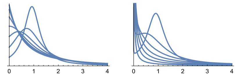
Figure 1: Probability densities of $R_{\alpha}^{\alpha}$ and $R_{\alpha}:=T_{\alpha}/T^{\prime}_{\alpha}$ for $\alpha=k/8,1\leq k\leq 7$. The $7$ densities of $R_{\alpha}^{\alpha}$ in the left panel are those of the scaled Cauchy variable $C_{\alpha}$ in (23) conditioned to be positive. The curves are identified by their values at $0$, which decrease as $\alpha$ increases, and their values at $1$ which increase with $\alpha$. The corresponding densities of $R_{\alpha}$ can be identified similarly in the right panel. By unimodality of the Cauchy density, in the left panel each density of $R_{\alpha}^{\alpha}$ is unimodal, with maximum density at $0$ for $\alpha\leq\mbox{$\frac{1}{2}$}$, and at $\sin(\alpha-\mbox{$\frac{1}{2}$})\pi$ for $\alpha\geq\mbox{$\frac{1}{2}$}$. Each density of $R_{\alpha}$ in the right panel has an infinite maximum achieved at $0+$. The discrimant of the quadratic (51) is $\Delta(\alpha):=2(\cos^{2}\alpha\pi+\alpha^{2}-1)$ which is negative for $\alpha\leq\alpha_{c}$, where $\alpha_{c}\approx 0.736484$ is the unique root $\alpha\in(0,1)$ of the equation $\Delta(\alpha)=0$. So the density of $R_{\alpha}$ is strictly decreasing for $\alpha\leq\alpha_{c}$, with strictly negative derivative for $\alpha<\alpha_{c}$, and with a unique point of inflection for $\alpha=\alpha_{c}$ at $(\sqrt{1-\alpha_{c}^{2}}/(1+\alpha_{c}))^{1/\alpha_{c}}\approx 0.278018$. For $\alpha>\alpha_{c}$, as for the top two curves with $\alpha=6/8$ and $\alpha=7/8$, the density of $R_{\alpha}$ is bimodal, with a local minimum at $r_{-}(\alpha)$ and a local maximum at $r_{+}(\alpha)$ where $r_{\pm}(\alpha):=(x_{\pm}(\alpha))^{1/\alpha}$ for $x_{\pm}(\alpha)$ the two roots in $[0,1]$ of the quadratic (51). A common feature of the laws of $R_{\alpha}^{\alpha}$ and $R_{\alpha}$ for all $0<\alpha<1$ is that each law has median $1$, due to $R_{\alpha}\stackrel{{\scriptstyle d}}{{=}}R_{\alpha}^{-1}$, and each law has infinite mean. As $\alpha\uparrow 1$, both laws converge to the distribution degenerate at $1$. But as $\alpha\downarrow 0$, the behavior is different. At each $x>0$, the density of $R_{\alpha}^{\alpha}$ converges to $(1+x)^{-2}$, which is the density of the limit in distribution of $R_{\alpha}^{\alpha}$. In parallel with this convergence, as $\alpha\downarrow 0$, the density of $R_{\alpha}$ converges pointwise to $0$, as the distribution of $R_{\alpha}$ converges vaguely to an atom of $\frac{1}{2}$ at $0$ and an atom of $\frac{1}{2}$ at $+\infty$. This pointwise convergence of densities as $\alpha\downarrow 0$ is apparent in both panels.

Figure 2: Discrimant and locations of the minimum and maximum of the density of $R_{\alpha}:=T_{\alpha}/T^{\prime}_{\alpha}$. Half the discriminant $\Delta(\alpha)$ of the quadratic equation (51) is $\cos^{2}\alpha\pi+\alpha^{2}-1$, as plotted in the left panel, with $\alpha_{c}\approx 0.736484$ the unique root of this function in $(0,1)$. The right panel shows the two graphs of $r_{\pm}(\alpha):=(x_{\pm}(\alpha))^{1/\alpha}$ for $x_{\pm}(\alpha)$ the two roots in $[0,1]$ of the quadratic equation (51), for $\alpha_{c}\leq\alpha<1$. The lower curve $r_{-}(\alpha)$ gives the location of the unique minimum in $(0,1)$ of the density of $R_{\alpha}$. This location decreases from $r_{\pm}(\alpha_{c})\approx 0.278018$ to $0$ as $\alpha$ increases from $\alpha_{c}$ to $1$. The upper curve $r_{+}(\alpha)$ is the location of the unique local maximum of the density $(0,\infty)$. This modal value is always less than $1$, and increases from $r_{\pm}(\alpha_{c})\approx 0.278018$ to the median value of $1$ as $\alpha$ increases from $\alpha_{c}$ to $1$.

3.3 Cauchy-Stieltjes transforms

For a real valued random variable $X$, the Cauchy-Stieltjes transform of $X$ is commonly defined to be the function of a complex variable $z$

$$G_{X}(z):={\mathbb{E}}(z-X)^{-1}\qquad(z\notin{\mathbb{R}}).$$ (52)

There are inversion formulas both for this transform, as well as for the generalized Cauchy-Stieltjes transform of $X$ of order $\theta$, say $G_{X,\theta}(z)$ obtained by replacing the power $-1$ in (52) by $-\theta$:

$$G_{X,\theta}(z):={\mathbb{E}}(z-X)^{-\theta}\qquad(z\notin{\mathbb{R}}).$$ (53)

See Demni (2016) for a recent article about this transform with references to earlier work. For $X$ with values in $[0,1]$ it is more pleasant to deal with the variant of this transform

$${\mathbb{E}}(1-\lambda X)^{-\theta}=\sum_{n=0}^{\infty}\frac{(\theta)_{n}}{n!}{\mathbb{E}}X^{n}\lambda^{n}=\lambda^{-\theta}G_{X,\theta}(\lambda^{-\theta})\qquad(|\lambda|<1)$$ (54)

where the series is convergent and equal to ${\mathbb{E}}(1-\lambda X)^{-\theta}$ for every $|\lambda|<1$ by dominated convergence. A distribution of $X$ on $[0,1]$ is uniquely determined by its moment sequence $({\mathbb{E}}X^{n},n=0,1,2,\ldots)$, hence also by its generalized Cauchy-Stieltjes transform of order $\theta$, for any fixed $\theta>0$. For unbounded non-negative $X$, including $X$ with ${\mathbb{E}}X=\infty$, for which there is not even a partial series expansion (54) for $\lambda$ in any neighbourhood of $0$, it is typically easier to work with

$${\mathbb{E}}(1+\lambda X)^{-\theta}=(-\lambda)^{\theta}G_{X,\theta}((-\lambda)^{-\theta})\qquad(\lambda\geq 0).$$ (55)

Here the left side is evidently a well defined and analytic function of $\lambda$ with positive real part. The right side may be understood by analytic continuation of $G_{X,\theta}(z)$ from non-real values of $z$. But arguments by analytic continuation can often be avoided by the following key observation. By introducing $\gamma(\theta)$ with gamma$(\theta)$ distribution, independent of $X$, and conditioning on $X$, the expectation in (55) is

$${\mathbb{E}}(1+\lambda X)^{-\theta}={\mathbb{E}}\exp[-\lambda\gamma(\theta)X]\qquad(\lambda\geq 0),$$ (56)

that is the ordinary Laplace transform of $\gamma(\theta)X$. This determines the distribution of $X$, by uniqueness of Laplace transforms, and the the following lemma which has been frequently exploited (Pitman and Yor, 2001, p. 358), Chaumont and Yor (2012, 1.13, 4.2, 4.24), (McKinlay, 2014, Theorem 3). As a general rule, in reading formulas involving generalized Stieltjes transforms of probability distributions of $X$, especially $X\geq 0$, matters are often simplified by interpreting the generalized Stieltjes transform as the Laplace transform of $\gamma(\theta)X$.

Lemma 4.

[Cancellation of independent gamma variables] For random variables or random vectors $X$ and $Y$, and $\gamma(\theta)$ with gamma$(\theta)$ distribution independendent of both $X$ and $Y$, for each real $a$ there is the equivalence of identities in distribution

$$\gamma(\theta)^{a}X\stackrel{{\scriptstyle d}}{{=}}\gamma(\theta)^{a}Y\qquad\iff\qquad X\stackrel{{\scriptstyle d}}{{=}}Y.$$ (57)

Proof.

Consider first the case of real random variables. Obviously ${\mathbb{P}}(\gamma(\theta)^{a}X\in B)={\mathbb{P}}(X\in B)$ if $B$ is any of the subsets $(-\infty,0)$, $\{0\}$ or $(0,\infty)$ of ${\mathbb{R}}$. So by conditioning it may as well be assumed that both $X$ and $Y$ are strictly positive, when there is no difficulty in taking logarithms. It is known (Gordon, 1994) that the distribution of $\log\gamma(\theta)$ is infinitely divisible, hence has a characteristic function which does not vanish. The conclusion in the univariate case follows easily, by characteristic functions. An appeal to the Cramér-Wold theorem takes care of the multivariate case. ∎

To illustrate these ideas, let us derive the ordinary Cauchy-Stieltjes transform of the ratio $R_{\alpha}:=T_{\alpha}/T^{\prime}_{\alpha}$ of two i.i.d. standard stable $(\alpha)$ variables, whose Mellin transform and probability density were already indicated above. From above, the problem is to calculate

$${\mathbb{E}}(1+\lambda R_{\alpha})^{-1}={\mathbb{E}}\exp(-\lambda\varepsilon T_{\alpha}/T^{\prime}_{\alpha})$$ (58)

for independent random variables $\varepsilon\stackrel{{\scriptstyle d}}{{=}}\gamma(1)$ and $T_{\alpha}\stackrel{{\scriptstyle d}}{{=}}T^{\prime}_{\alpha}$. But we already know from (46) that $\varepsilon/T^{\prime}_{\alpha}\stackrel{{\scriptstyle d}}{{=}}\varepsilon^{1/\alpha}$. So

$${\mathbb{E}}(1+\lambda R_{\alpha})^{-1}={\mathbb{E}}\exp(-\lambda\varepsilon^{1/\alpha}T_{\alpha})={\mathbb{E}}\exp(-\lambda^{\alpha}\varepsilon)=(1+\lambda^{\alpha})^{-1}.$$ (59)

Thus the distribution of $R_{\alpha}$ is uniquely characterized by the simple Cauchy-Stieltjes transform

$${\mathbb{E}}(1+\lambda R_{\alpha})^{-1}=(1+\lambda^{\alpha})^{-1}\qquad(\lambda>0).$$ (60)

It is notable that the explicit formula (50) for the density of $R_{\alpha}$ with Laplace-Stieltjes transform $(1+\lambda^{\alpha})^{-1}$ is much simpler than the corresponding inversion for the common distribution of $\varepsilon R_{\alpha}\stackrel{{\scriptstyle d}}{{=}}\varepsilon R_{\alpha}^{-1}\stackrel{{\scriptstyle d}}{{=}}\varepsilon^{1/\alpha}T_{\alpha}$ which has $(1+\lambda^{\alpha})^{-1}$ as its ordinary Laplace transform:

$${\mathbb{P}}(\varepsilon R_{\alpha}>x)=E_{\alpha}(-x^{\alpha})\qquad(x\geq 0)$$ (61)

where

$$E_{\alpha}(z):=\sum_{k=0}^{\infty}\frac{z^{k}}{\Gamma(k\alpha+1)}\qquad(z\in{\mathbb{C}})$$

is the classical Mittag-Leffler function with parameter $\alpha$. This is an entire function of $z\in{\mathbb{C}}$, for each $\alpha\in{\mathbb{C}}$ with strictly positive real part, with $\alpha\in(0,1)$ here. This formula was found by Pillai (1990). See also (Mainardi et al., 2001, (3.9) and (4.37)) for closely related transforms, and Gorenflo et al. (2014) for a recent survey of Mittag-Leffler functions and their applications. Compare also with the density of $T_{\alpha}$, given by Pollard (1946)

$${\mathbb{P}}(T_{\alpha}\in dt)/dt=\frac{1}{\pi}\sum_{k=0}^{\infty}\sin(\alpha k\pi)\frac{(-1)^{k+1}\Gamma(k\alpha+1)}{k!\,t^{k\alpha+1}}.$$ (62)

Only for $\alpha=\mbox{$\frac{1}{2}$}$, when $T_{\mbox{$\frac{1}{2}$}}\stackrel{{\scriptstyle d}}{{=}}1/(2\gamma(\mbox{$\frac{1}{2}$}))$ is there substantial simplification of this series formula. But see Penson and Górska (2010) for explicit expressions for the density (62) in terms of the Meijer $G$ function for rational $\alpha$, and Schneider (1986) for a general representation of stable densities in terms of Fox functions. See also Ho et al. (2007).

Returning to the context of random discrete distributions, if $P_{\alpha,0}$ is governed by the $(\alpha,0)$ model defined by normalizing the jumps of a stable$(\alpha)$ subordinator on some fixed interval of length say $s>0$, then it is evident that for $X=X_{p}$ the indicator of an event of probability $p$, the distribution of the $P_{\alpha,0}$ mean of $X_{p}$ is determined by

$$M_{\alpha,0}(X_{p})\stackrel{{\scriptstyle d}}{{=}}\frac{T_{\alpha}(p)}{T_{\alpha}(1)}\stackrel{{\scriptstyle d}}{{=}}\frac{p^{1/\alpha}T_{\alpha}}{p^{1/\alpha}T_{\alpha}+q^{1/\alpha}T^{\prime}_{\alpha}}\stackrel{{\scriptstyle d}}{{=}}\frac{1}{1+cR_{\alpha}}$$ (63)

where $(T_{\alpha}(s),s\geq 0)$ is the stable$(\alpha)$ subordinator with $T_{\alpha}(s)\stackrel{{\scriptstyle d}}{{=}}s^{1/\alpha}T_{\alpha}$ for $T_{\alpha}$ the standard stable$(\alpha)$ variable as above, and $c:=(q/p)^{1/\alpha}$ for $q:=1-p$. Here the second $\stackrel{{\scriptstyle d}}{{=}}$ appeals to the decomposition of $T_{\alpha}(1)$ into two independent components $T_{\alpha}(1)=T_{\alpha}(p)+(T_{\alpha}(1)-T_{\alpha}(p))$ with $T_{\alpha}(p)\stackrel{{\scriptstyle d}}{{=}}p^{1/\alpha}T_{\alpha}$ and $T_{\alpha}(1)-T_{\alpha}(p)\stackrel{{\scriptstyle d}}{{=}}q^{1/\alpha}T_{\alpha}$. The distribution of $M_{\alpha,0}(X_{p})$ is thus obtained from that of $R_{\alpha}$ by a simple change of variable. Moreover, for any real $X$, the identity

$$\left(1+\frac{\lambda}{1+cX}\right)^{-1}=1-\frac{\lambda}{(1+\lambda)}\left(1+\frac{cX}{(1+\lambda)}\right)^{-1}$$

allows the Cauchy-Stieltjes transform of $(1+cX)^{-1}$ to be expressed directly in terms of that of $X$. In particular, for the ratio of independent stable variables $X=R_{\alpha}$ with the simple Cauchy-Stieltjes transform (60), and $c:=(q/p)^{1/\alpha}$ with $q:=1-p$, this algebra simplifies nicely to give in (63)

$${\mathbb{E}}(1+\lambda M_{\alpha,0}(X_{p}))^{-1}=\frac{q+p(1+\lambda)^{\alpha-1}}{q+p(1+\lambda)^{\alpha}}.$$ (64)

This is the Stieltjes transform (20) found by Lamperti. See (Pitman and Yor, 1997b, §4) for further discussion.

4 Some basic theory of $P$-means

This section presents some general theory of $P$-means, for an arbitrary random discrete distribution $P$, and its relation to Kingman’s theory of partition structures, relying only the simplest examples to motivate the development. This postpones to Section 5.7 the study of the rich collection of examples associated with the $(\alpha,\theta)$ model.

4.1 Partition structures

Kingman (1978) introduced the concept of the partition structure associated with sampling from a random probability distribution $F$. That is, the collection of probability distributions of the random partitions $\Pi_{n}$ of the set $[n]:=\{1,\ldots,n\}$, generated by a random sample $Y_{1},\ldots,Y_{n}$ from $F$, meaning that conditionally given $F$ the $Y_{i}$ are i.i.d. according $F$. The blocks of $\Pi_{n}$ are the equivalence classes of the restriction to $[n]$ of the random equivalence relation $i\sim j$ iff $Y_{i}=Y_{j}$. A convenient encoding of this partition structure is provided by its exchangeable partition probability function (EPPF) (Pitman, 1995). This is a function $p$ of compositions $(n_{1},\ldots,n_{k})$ of $n$, that is to say sequences of $k$ positive integers $(n_{1},\ldots,n_{k})$ with $\sum_{i=1}^{k}n_{i}=n$ for some $1\leq k\leq n$. The function $p(n_{1},\ldots,n_{k})$ gives, for each particular partition $\{B_{1},\ldots,B_{k}\}$ of $[n]$ into $k$ blocks, the probability

$${\mathbb{P}}(\Pi_{n}=\{B_{1},\ldots,B_{k}\})=p(\#B_{1},\ldots,\#B_{k}),$$ (65)

where $\#B_{i}$ is the size of the block $B_{i}$ of indices $j$ with the same value of $Y_{j}$. A random partition $\Pi_{n}$ of $[n]$ is called exchangeable iff its distribution is invariant under the natural action of permutations of $[n]$ on partitions of $[n]$. Equivalently, its probability function is of the form (65) for some function $p(n_{1},\ldots,n_{k})$ that is non-negative and symmetric. The sum of these probabilities (65), over all partitions $\{B_{1},\ldots,B_{k}\}$ of $[n]$ into various numbers $k$ of blocks, must then equal $1$. This constraint is most easily expressed in terms of the associated exchangeable random composition of $n$

$$N^{\rm ex}_{\bullet:n}:=(N^{\rm ex}_{1:n},N^{\rm ex}_{2:n},\ldots,N^{\rm ex}_{K_{n}:n})$$

defined by listing the sizes of blocks of $\Pi_{n}$ in an exchangeable random order. This means that conditionally given the number $K_{n}$ of components of $\Pi_{n}$ equals $k$ for some $1\leq k\leq n$, and that $\Pi_{n}=\{B_{1},\ldots,B_{k}\}$ for some particular sequence of blocks $(B_{1},\ldots,B_{k})$, which may be listed in any order, for instance their order of least elements, $N^{\rm ex}_{\bullet:n}:=\#B_{\sigma(1)},\ldots,\#B_{\sigma(k)}$ where $\sigma$ is a uniform random permutation of $[k]$. As indicated in Pitman (2006, (2.8)), the usual probability function of this random composition of $n$ is the exchangeable composition probability function (ECPF)

$${\mathbb{P}}(N^{\rm ex}_{\bullet:n}=(n_{1},\ldots,n_{k}))=p^{\rm ex}(n_{1},\ldots,n_{k}):=\frac{1}{k!}\binom{n}{n_{1},\ldots,n_{k}}p(n_{1},\ldots,n_{k}).$$ (66)

These probabilities must sum to $1$ over all compositions of $n$. So the normalization condition on an EPPF is that for $p^{\rm ex}$ derived from $p$ using the multiplier in (66),

$$\sum_{k=1}^{n}\sum_{(n_{1},\ldots,n_{k})}p^{\rm ex}(n_{1},\ldots,n_{k})=1.$$ (67)

Here and in similar sums below, $(n_{1},\ldots,n_{k})$ ranges over the set of $\binom{n-1}{k-1}$ compositions of $n$ into $k$ parts. To understand (66), observe that putting the components of $\Pi_{n}$ in an exchangeable random order creates a random ordered partition of $[n]$, with block sizes $N^{\rm ex}_{\bullet:n}$. So ${\mathbb{P}}(N^{\rm ex}_{\bullet:n}:=(n_{1},\ldots,n_{k}))$ is the sum, over all ordered partition of $[n]$ into $k$ blocks of the specified sizes, of the probability of each ordered partition of those sizes. Each particular ordered partition has probability $p(n_{1},\ldots,n_{k})/k!$, and the number of these ordered partitions with sizes $(n_{1},\ldots,n_{k})$ is the multinomial coefficient.

For $\Pi_{n}$ generated by sampling from a random discrete distribution with atoms of sizes $(P_{j})$, let $(J_{1},\ldots,J_{n})$ denote the corresponding sample of positive integer indices. Then for each particular partition $\{B_{1},\ldots,B_{k}\}$ of $[n]$ as in (65)

$${\mathbb{P}}\left((\Pi_{n}=\{B_{1},\ldots,B_{k}\})\bigcap_{i=1}^{k}\bigcap_{\ell\in B_{i}}(J_{\ell}=j_{i})\right)={\mathbb{E}}\prod_{i=1}^{k}P_{j_{i}}^{n_{i}}\mbox{ with }n_{i}:=\#B_{i}.$$

Hence, by conditioning on $P$,

$$p(n_{1},\ldots,n_{k}):=\sum_{(j_{1},\ldots,j_{k})}{\mathbb{E}}\prod_{i=1}^{k}P_{j_{i}}^{n_{i}}.$$ (68)

where the sum is over all sequences of $k$ distinct positive integers $(j_{1},\ldots,j_{k})$. As observed by Kingman, as $n$ varies, the partition structure associated with sampling from a random distribution is subject to a consistency condition: the restriction of $\Pi_{n+1}$ to $[n]$ must be $\Pi_{n}$ for every $n\geq 1$. In terms of the EPPF, this consistency condition implies

$$p({\bf n})=\sum_{i=1}^{k+1}p({\bf n}^{(i+)})$$ (69)

where ${\bf n}=(n_{1},\ldots,n_{k})$ ranges over compositions of $n$, and ${\bf n}^{(i+)}$ for $1\leq i\leq k+1$ is ${\bf n}$ with the $i$th component incremented by $1$, meaning for $({\bf n},1)$ obtained by appending a $1$ to ${\bf n}$ for $i=k+1$. See Pitman (2006, §3.2) for further discussion.

The instance of the general formula (3), when $(S,\SS)$ is the unit interval $[0,1]$ with Borel sets, and the $Y_{j}=U_{j}$ are i.i.d. uniform $[0,1]$ variables, independent of $P$, is of particular importance. Write $F_{P}$ for the random probability measure on $[0,1]$ which sprinkes the atoms of $P$ at i.i.d. uniform random locations. So by definition, for all bounded or non-negative measurable $g$

$$\int_{0}^{1}g(u)F_{P}(du)=M_{P}(g(U)):=\sum_{j=1}^{\infty}g(U_{j})P_{j}$$ (70)

In particular, for $g(u)=1(u\leq v)$, the indicator of the interval $[0,v]$, the random cumulative distribution function (c.d.f.) of $F_{P}$ is

$$F_{P}[0,v]:=M_{P}(1(U\leq v)):=\sum_{j=1}^{\infty}1(U_{j}\leq v)P_{j}\qquad(0\leq v\leq 1).$$ (71)

Note that $F_{P}[0,0]=0$ and $F_{P}[0,1]=1$ almost surely.

The following proposition summarizes some well known facts:

Proposition 5.

[Kallenberg (1973), Kingman (1978)] The random c.d.f. $F(v):=F_{P}[0,v]$, derived as above for $0\leq v\leq 1$ from a random discrete distribution $P$, is a process with exchangeable increments, meaning that for each $m=1,2,\ldots$ the sequence $(F(i/m)-F((i-1)/m),1\leq i\leq m)$ is exchangeable. The collection of distributions of these exchangeable sequences is an encoding of the partition structure generated by $P$, as is the collection of finite-dimensional distributions of $P^{\downarrow}$, the ranked re-ordering of $P$, and the collection of finite-dimensional distributions of $P^{*}$, the size-biased permutation of $P$. In other words, for two random discrete distributions $P$ and $Q$, with associated random c.d.f.s with exchangeable increments $F_{P}$ and $F_{Q}$, and exchangeable partition probability functions $p_{P}$ and $p_{Q}$, the following conditions are equivalent:

• ${P^{\downarrow}}\stackrel{{\scriptstyle d}}{{=}}{Q^{\downarrow}}$

• $P^{*}\stackrel{{\scriptstyle d}}{{=}}Q^{*}$

• $p_{P}({\bf n})=p_{Q}({\bf n})$ for all compositions of positive integers ${\bf n}$;

• $F_{P}$ and $F_{Q}$ share the same finite dimensional distributions.

Proof.

As indicated by Kallenberg, the finite-dimensional distributions of $F=F_{P}$ determine those of the list $P^{\downarrow}$ of ranked jumps of $P$, and conversely. It is obvious that the laws of $P^{\downarrow}$ and $P^{*}$ determine each other, and that either of these laws determines the EPPF $p_{P}$, by application of formula (68) with $P$ replaced by $P^{\downarrow}$ or $P^{*}$. That the law of $P^{\downarrow}$ can be recovered from the partition structure was shown by Kingman (1978). ∎

See also Pitman (2006, Theorem 3.1) for an explicit formula expressing the EPPF in terms of product moments derived from $P^{*}$.

A nice exercise in Kallenberg’s encoding of $P$ by an exchangeable random c.d.f. $F:=F_{P}$ is provided by the following construction, proposed by Patil and Taillie (1977, Example 2.10), in an insightful review article which appeared a year before the general theory of partition structures was offered by Kingman (1978). Suppose $P$ is a random discrete distribution with ${\mathbb{P}}(P_{i}>0)=1$ for each $i=1,2,\ldots$. Let $(U_{i})$ be a sequence of i.i.d. uniform variables, independent of $P$, and for each $0<p<1$ consider the sequence $P_{i}1(U_{i}\leq p)$ obtained by annihilating each $P_{i}$ with $U_{i}>p$ and keeping each $P_{i}$ with $U_{i}\leq p$. Then a new random discrete distribution $P(p)$, called a $p$-thinning or $p$-screening of $P$, is obtained by ignoring the annihilated entries $P_{i}$ with $U_{i}>p$, and listing the remaining entries of $P_{i}$ with $P_{i}\leq p$ in their original order, renormalized by their sum $F(p):=\sum_{i}P_{i}1(U_{i}\leq p)$. More precisely, the $j$th entry of $P(p)$ is $P_{j}(p):=P_{\tau(p,j)}/F(p)$ where $\tau(p,j)$ is the $j$th index $i$ with $U_{i}\leq p$. So $\tau(p,j)$ is the sum of $j$ independent copies of $\tau(p,1)$ with the geometric$(p)$ distribution ${\mathbb{P}}(\tau(p,1)=k)=pq^{k-1}$ for $q:=1-p$, and the sequence of indices $(\tau(p,j),j=1,2,\ldots)$ is independent of $P$. In terms of the random c.d.f. with exchangeable increments $F(u):=\sum_{i}P_{i}1(U_{i}\leq u)$, whose jumps in some order are the $P_{i}$, the $p$-thinning $P(p)$ is by construction a listing of jumps of the random c.d.f. with exchangeable increments $(F(up)/F(p),0\leq u\leq 1)$. In terms of $P$-means, for suitable distributions of $X$, the $P(p)$-mean of $X$ is the ratio of two jointly distributed $P$-means:

$$M_{P(p)}(X)=\frac{M_{P}(X1(U\leq p))}{M_{P}(1(U\leq p))}:=\frac{\sum_{i}X_{i}1(U_{i}\leq p)P_{i}}{\sum_{i}1(U_{i}\leq p)P_{i}}.$$ (72)

A particularly appealing instance of this construction is described by the following proposition:

Proposition 6.

(Patil and Taillie, 1977, Theorem 2.5) If $P$ is governed by the GEM$(0,\theta)$ model $P_{j}:=H_{j}\prod_{i=1}^{j-1}H_{i}$ for i.i.d. random factors $H_{i}$ with $H_{i}\stackrel{{\scriptstyle d}}{{=}}\beta_{1,\theta}$ for some $\theta>0$, then

• the random fraction $F(p)$ has beta$(p\theta,q\theta)$ distribution for $q:=1-p$;

• the $p$-thinned random discrete distribution $P(p)$ has GEM$(0,p\theta)$ distribution;

• the fraction $F(p)$ is independent of the random discrete distribution $P(p)$.

Proof.

As indicated by Patil and Taillie, this is a consequence of the representation of $P$ by random sampling from the random c.d.f. $F(u)=\gamma(u\theta)/\gamma(\theta)$ derived from the standard gamma subordinator. See Pitman (2006, §4.2) for a proof of McCloskey’s result that the size-biased representation of jumps of this $F$ gives $P$ governed by the GEM$(0,\theta)$ model with i.i.d. beta$(1,\theta)$ distributed residual factors. Granted the gamma representation of $P$, part (i) is just the basic beta-gamma algebra (6). Part (ii) holds by the identification of $F(up)/F(p)=\gamma(up\theta)/\gamma(p\theta),0\leq u\leq 1$ as the c.d.f. with exchangeable increments associated with $P(p)$. Part (iii) appeals to independence part (7) of the beta-gamma algebra, which makes $F(p)=\gamma(p\theta)/\gamma(\theta)$ independent of the process $(F(up)/F(p),0\leq u\leq 1)$, hence also independent of its list of jumps $P(p)$ in their order of discovery by a process of uniform random sampling. ∎

As remarked by Patil and Taillie, the above proposition holds also with GEM$(0,\theta)$ replaced by its decreasing rearrangement, the Poisson-Dirichlet $(0,\theta)$ distribution. Various components of the proposition can be broken down and generalized as follows.

Proposition 7.

Let $P(p)$ be the random discrete distribution obtained by $p$-thinning of a random discrete distribution $P$ with ${\mathbb{P}}(P_{i}>0)=1$ for each $i=1,2,\ldots$.

• if $P=P^{\downarrow}$ is in ranked order, then so is $P(p)$;

• if $P=P^{*}$ is in size-biased random order, then so is $P(p)$;

Suppose $P$ is a list of jumps of the random c.d.f. $F$ with exchangeable increments defined by normalization of a subordinator $A$, say $F(u)=A(\theta u)/A(\theta),0\leq u\leq 1$, for some fixed $\theta>0$, then

• $P(p)$ is a list of normalized jumps of the same subordinator on the interval $[0,p\theta]$ instead of $[0,\theta]$.

• if $P$ is in either ranked or size-biased order, then the following two conditions are equivalent:

  $$P(p)\stackrel{{\scriptstyle d}}{{=}}P\mbox{ for every }0<p<1;$$ (73)

  $$A (\alpha) 0<\alpha<1$$ is a stable subordinator for some . (74)

  in which case $P^{*}$ is governed by the GEM$(\alpha,0)$ model with independent residual factors $H_{i}\stackrel{{\scriptstyle d}}{{=}}\beta_{1-\alpha,i\alpha}$ for $i=1,2,\ldots$.

Proof.

Part (i) is obvious. To see part (ii), observe that $P=P^{*}$ may be constructed by listing the jumps of the associated random c.d.f. with exchangeable increments $F$ in the order they are discovered by a process of random sampling from $F$. But then by construction as above, $P(p)$ is the list of sizes of jumps of $F$ in $[0,p]$, relative to their sum $F(p)$, in the order of their discovery in samping from $F$. But the successive values of the sample from $F$ which fall in $[0,p]$ form a sample from $F$ conditioned on $[0,p]$. Thus $P(p)$ is just the list of atoms of this random conditional distribution in their order of their discovery by a process of random sampling, and it follows that $P(p)$ is in size-biased random order. Part (iii) is just a reprise of part (ii) of the previous proposition, with a general subordinator instead of the gamma process. As for part (iv), if $F$ is derived from a stable subordinator, it is easily seen that the distribution of the process $(F(up)/F(p)=A(up)/A(p),0\leq u\leq 1)$ does not depend on $p$. Hence $P(p)\stackrel{{\scriptstyle d}}{{=}}P$, for either ranked or size-biased ordering of $P$, by (i) and (ii). Conversely, it is known (Pitman and Yor, 1992, Lemma 7.5) that for a subordinator $A$ the distribution of $A(1)$ is determined up to a scale factor by that of the process $(A(u)/A(1),0\leq u\leq 1)$. If $P(p)\stackrel{{\scriptstyle d}}{{=}}P$ for all $0<p<1$, then the distribution of $(F(up)/F(p)=A(up)/A(p),0\leq u\leq 1)$ is the same for all $0<p<1$, hence $A(p)\stackrel{{\scriptstyle d}}{{=}}c(p)A(1)$ for some constant $c(p)$. It is well known that for a subordinator $A$ this condition implies that $A$ is stable with some index $\alpha\in(0,1)$ as indicated in (74). ∎

The only part of Proposition 6 which does not extend to a subordinator more general than the gamma process is the independence of $F(p)$ and $P(p)$. This is a consequence of independence of $A(t)$ and $(A(ut)/A(t),0\leq u\leq t)$, which is well known to be a characteristic property of $A(t)=a\gamma(bt)$ for some $a,b>0$. See Pitman (2006, §4.2) and work cited there. See also Pitman (2003) and Émery and Yor (2004) for more about bridges with exchangeable increments obtained by normalizing a subordinator.

The construction of infinitely divisible semi-stable laws by Lévy (1954, §58) shows for each fixed $q\in(0,1)$ there exist non-stable subordinators such that (73) holds if $p=q^{n}$ for some $n=1,2,\ldots$ but not for all $0<p<1$. Let $P_{(\alpha,0)}$ denote a random discrete distribution governed by the $(\alpha,0)$ model, say in size-biased order for simplicity, but it could just as well be ranked. Part (iv) of the above proposition implies that for each probability distribution $\pi$ on $(0,1)$, which might be regarded as a prior distribution on the stability index $\alpha$, the formula

$${\mathbb{P}}(P\in\bullet)=\int_{(0,1)}\pi(d\alpha){\mathbb{P}}(P{(\alpha,0)}\in\bullet)$$ (75)

defines a mixture of $(\alpha,0)$ laws, which governs $P$ with the invariance property (73) under $p$-thinning for all $0<p<1$.

Problem 8.

Are there any other laws besides (75) of random discrete distributions $P$ such that ${\mathbb{P}}(P_{i}>0)=1$ for all $i$ and $P(p)\stackrel{{\scriptstyle d}}{{=}}P$ for all $0<p<1$?

See Pitman (1999) and Bertoin and Pitman (2000) for various constructions of $P_{(\alpha,0)}$ governed by the $(\alpha,0)$ model as a stochastic process indexed by $\alpha\in(0,1)$.

4.2 $P$-means and partition structures

The present point of view is that the collection of distributions of $P$-means $M_{P}(X)$, indexed by various distributions of $X$, should be regarded as yet another encoding of the partition structure associated with $P$. That point of view is justified by the following corollary of Proposition 5, which does not seem to have been pointed out before. Call a random variable simple if it takes only a finite number of possible values.

Corollary 9.

[Characterization of partition structures by $P$-means] For each random discrete distribution $P$, the collection of distributions of its $P$-means $M_{P}(X)$, as $X$ ranges over simple random variables, is an encoding of the partition structure of $P$. That is to say, for any two random discrete distributions $P$ and $Q$, the condition

• $M_{P}(X)\stackrel{{\scriptstyle d}}{{=}}M_{Q}(X)$ for every simple $X$

can be added to the list of equivalent conditions in the Proposition 5.

Proof.

As remarked earlier around (21), it the distribution of $M_{P}(X)$ remains unchanged if $P$ is replaced by $P^{\downarrow}$, and the same for $Q$ instead of $P$. So $P^{\downarrow}\stackrel{{\scriptstyle d}}{{=}}Q^{\downarrow}$ implies $M_{P}(X)\stackrel{{\scriptstyle d}}{{=}}M_{Q}(X)$. For the converse, the Cramér-Wold theorem shows that the finite-dimensional distributions of $F_{P}$ are determined by the collection of one-dimensional distributions of finite linear combinations of $F_{P}[0,v],0\leq v\leq 1$, each of which is a $P$-mean by application of (70):

$$\sum_{i}\,a_{i}\,F_{P}[0,v_{i}]=M_{P}\left(\sum_{i}\,a_{i}1(U\leq v_{i})\right).$$

So $M_{P}(X)\stackrel{{\scriptstyle d}}{{=}}M_{Q}(X)$ for all simple $X$ implies that the finite dimensional distributions of $F_{P}$ and $F_{Q}$ are the same. Hence the conclusion, by the preceding proposition. ∎

Part of how the partition structure of $P$ is determined by the distributions of $P$-means $M_{P}(X)$, as the distribution of $X$ varies, is found by consideration of the $P$-means of indicator variables $X$, that is $X=1(U\leq v)$ whose $P$-mean is $F_{P}(v)$. So there is the following proposition, which also does not seem to have been noticed before, though it is the easiest case for an indicator variable of the general moment formula for $P$-means, due to Kerov, which is presented later in Corollary 22.

Proposition 10.

Let $F(v):=F_{P}[0,v]$ be the random cumulative distribution function with exchangeable increments on $[0,1]$ derived from a random discrete distribution $P$, and let $K_{n}$ be the number of distinct values in a random sample of size $n$ from either $P$ or from $F$. Then the $n$th moment of $F(v)$ is a polynomial in $v$ of degree at most $n$, which equals the probability generating function of $K_{n}$ evaluated at $v$:

$${\mathbb{E}}[F(v)]^{n}={\mathbb{E}}v^{K_{n}}=\sum_{k=1}^{n}{\mathbb{P}}(K_{n}=k)v^{k}$$ (76)

where ${\mathbb{P}}(K_{n}=k)$ is determined by the ECPF $p^{\rm ex}$ of $P$ according to the formula

$${\mathbb{P}}(K_{n}=k)=\sum_{(n_{1},\ldots,n_{k})}p^{\rm ex}(n_{1},\ldots,n_{k})$$ (77)

where the sum is over all $\binom{n-1}{k-1}$ compositions of $n$ into $k$ parts. Consequently, the collection of one-dimensional distributions of $K_{n}$, for $n=1,2,\ldots$ determines the collection of one-dimensional distributions of $F(v)$ for $0\leq v\leq 1$, and vice versa.

Proof.

Formula (76) displays two different ways of evaluating the probability of the event $E:=\cap_{1\leq i\leq n}(V_{i}\leq v)$ for a random sample $V_{1},\ldots,V_{n}$ from $F$. On the one hand, ${\mathbb{P}}(E\,|\,F)=[F(v)]^{n}$. On the other hand, ${\mathbb{P}}(E\,|\,K_{n}=k)=v^{k}$, because given $k$ distinct values of the $V_{i}$, these values are $k$ independent uniform $[0,1]$ variables $U_{j},1\leq j\leq k$, which all fall to the left of $v$ with probability $v^{k}$. ∎

It is known (Nacu, 2006) that another equivalent condition is equality in distribution of the two sequences $(K_{n},n\geq 1)$ generated by sampling from $P$ and $Q$ respectively.

Problem 11.

Does equality of the one-dimensional distributions of $K_{n}$, generated by sampling from $P$ and $Q$ for each $n$, imply equality of partition structures?

By Corollary 10, this condition is the same as equality of one-dimensional distributions of $F_{P}[0,p]$ and $F_{Q}[0,p]$ for each $0\leq p\leq 1$. So the issue is whether the finite-dimensional distributions of an increasing process with exchangeable increments are determined by its one-dimensional distributions. [Kallenberg (1973), established a result in this vein, that the distribution of any process on $[0,1]$ with exchangeable increments and continuous paths is determined by its one-dimensional distributions.

It appears that the distribution of an exchangeable random partition $\Pi_{n}$ on $[n]$, with restrictions $\Pi_{m}$ to $[m]$ for $m\leq n$, is determined by the collection of distributions of $K_{m}$, the number of blocks of $\Pi_{m}$, for $1\leq m\leq n$, for $n\leq 11$ but not for $n=12$. To see this, consider the $\#_{\rm part}(n)$ probabilities of individual partitions of $n$ in the distribution of the partition of $n$ induced by the ranked block sizes of $\Pi_{n}$, where $\#_{\rm part}(n)$ is the number of partitions of $n$. These $\#_{\rm part}(n)$ probabilities are subject only to the constraints of being non-negative, with sum $1$, so the range of $\#_{\rm part}(n)-1$ of these probabilities contains some open ball in ${\mathbb{R}}^{\#_{\rm part}(n)-1}$. The ${\mathbb{P}}(K_{m}=k)$ for $1\leq k<m\leq n$ then form a collection of $\binom{n-1}{2}$ linearly independent linear combinations of the $\#_{\rm part}(n)$. It is easily checked that $\#_{\rm part}(n)-1\leq\binom{n-1}{2}$ for $1\leq n\leq 11$, but $\#_{\rm part}(12)-1=76>66=\binom{12}{2}$. Hence the conclusion. However, it does not seem at all obvious how to construct such an example which is part of an infinite partition structure derived by sampling from a random discrete distribution.

The following proposition develops the meaning of the terms $p^{\rm ex}(n_{1},\ldots,n_{k})$ in the sum (77) for ${\mathbb{P}}(K_{n}=k)$, in the context of the preceding proof.

Proposition 12.

Let $V_{1},\ldots,V_{n}$ be a sample from $F_{P}$, meaning that

$${\mathbb{P}}\left(\cap_{i=1}^{n}(V_{i}\leq v_{i})\,|\,F_{P}\right)=\prod_{i=1}^{n}F_{P}[0,v_{i}]\qquad(0\leq v_{i}\leq 1).$$ (78)

Let $K_{n}$ be the number of distinct values among $V_{1},\ldots,V_{n}$, and let $N^{\rm ex}_{\bullet:n}$ be the numbers of repetitions of these values in the sample $V_{1},\ldots,V_{n}$, in increasing order of $V$-values. Then $N^{\rm ex}_{\bullet:n}$ is an exchangeable random composition of $n$ with the probability function $p^{\rm ex}$ featured in formulas (66) and (77).

Proof.

By construction, $K_{n}$ is the number of blocks of $\Pi_{n}$, the random partition of $[n]$ generated by sampling from $P$. On the event of probability one that there are no ties among the $U$-values, the association $V_{i}=U_{J_{i}}$ pairs distinct $V$-values with distinct $J$-values in a sample $J_{1},\ldots,J_{n}$ of indices of $P$. Thus $K_{n}$ is the number of distinct values in a sample of size $n$ from $P$, and the distinct $V$-values are the uniform order statistics

$$U_{1:K_{n}}<U_{2:K_{n}}<\cdots<U_{K_{n}:K_{n}}$$

where for $k=1,2,\ldots$ the $U_{1:k}<U_{2:k}<\cdots<U_{k:k}$ are the order statistics of the first $k$ i.i.d. uniform variables $U_{1},\ldots,U_{k}$. It is well known that $U_{i}=U_{\sigma_{k}(i):k}$ for a random permutation $\sigma_{k}$ of $[k]$ that is independent of these $k$ order statistics. Hence $N^{\rm ex}_{\bullet:n}$ is an exchangeable random composition whose probability function (66) encodes the partition structure of $P$. ∎

4.3 $P$-means as conditional expectations

The point of view taken here is that a random discrete distribution $P$ may be regarded as a probabilistic mechanism for turning a suitable random variable $X$ into another random variable $M_{P}(X)$. Considered in this way, $M_{P}$ becomes an operator on random variables $X$, whose properties are those of a conditional expectation operator. In the first instance, the definition $M_{P}(X):=\sum_{j}X_{j}P_{j}$, makes $M_{P}$ an operator on probability distributions, which converts the common distribution of $X$ and the $X_{j}$ into the distribution of the new random variable $M_{P}(X)$. There is no specification of which of the many identically distributed variables $X_{j}$ should be regarded as $X$.

This construction of ${\widetilde{X}}:=M_{P}(X)$ puts ${\widetilde{X}}$ on the same probability space as all the copies $X_{j}$ of $X$. But the joint distribution of ${\widetilde{X}}$ and $X_{j}$ will typically depend on $j$. So there is no well defined joint distribution of ${\widetilde{X}}$ and a generic representative $X$ of the terms $X_{j}$ without some further precision. For instance, if ${\mathbb{E}}(X)=0$ and ${\mathbb{E}}X^{2}<\infty$, then the covariance

$${\mathbb{E}}({\widetilde{X}}X_{j})=({\mathbb{E}}P_{j}){\mathbb{E}}X^{2}$$

will typically depend on $j$. Only exceptionally, as in the case of exchangeable $P_{1},\dots,P_{m}$, does the joint law of $({\widetilde{X}},X_{j})$ not depend on $j$ for some finite range $1\leq j\leq m$. This apparent lack of a joint distribution of $X$ and ${\widetilde{X}}:=M_{P}(X)$ should be contrasted with conditional expectations ${\widetilde{X}}:={\mathbb{E}}(X\,|\,\mathcal{G})$ for $\mathcal{G}$ any sub $\sigma$-field of events in a probability space $(\Omega,\mathcal{F},{\mathbb{P}})$ on which $X$ is defined and integrable. For then ${\widetilde{X}}$ and $X$ are defined on the same probability space, with an induced joint probability distribution ${\mathbb{P}}((X,{\widetilde{X}})\in\bullet)$ on ${\mathbb{R}}^{2}$.

There are however many indications in the literature of particular $P$-means, that the operation which transforms a random variable $X$ into $M_{P}(X)$ shares properties of a conditional expectation operator ${\mathbb{E}}(X\,|\,\mathcal{G})$. Most obviously, $M_{P}$ is a positive operator: $X\geq 0$ implies $M_{P}(X)\geq 0$, and $M_{P}$ is a linear operator, meaning that if $(X,Y)$ has some arbitrary joint distribution, such that both ${\widetilde{X}}:=M_{P}(X)$ and ${\widetilde{Y}}:=M_{P}(Y)$ are well defined almost surely, then the natural construction of a random pair $({\widetilde{X}},{\widetilde{Y}}):=M_{P}(X,Y)$, using one copy of $P$ and an i.i.d. sequence $(X_{j},Y_{j})$ of copies of $(X,Y)$, makes

$$M_{P}(aX+bY)=aM_{P}(X)+bM_{P}(Y).$$

It is also easily shown there is a monotone convergence theorem for $P$-means: with the same coupling construction

$$0\leq X_{n}\uparrow X n\to\infty 0\leq M_{P}(X_{n})\uparrow M_{P}(X)$$ as implies a.s. (79)

All of which supports the idea that $P$-means should be regarded as some kind of conditional expectation operator. In fact, for any prescribed distribution of $X$ on an abstract measurable space, there is the following canonical construction of $X$ jointly with a sequence of i.i.d. copies $(X_{j})$ of $X$ and a random discrete $P$ with any desired distribution, and a suitable $\sigma$-field of events $\mathcal{G}$, which makes

$$M_{P}[g(X)]={\mathbb{E}}[g(X)\,|\,\mathcal{G}]\qquad a.s.$$

for all bounded or non-negative measurable functions $g$. Assume that the $(X_{j})$ and $(P_{j})$ are defined together with a uniform $[0,1]$ variable $U$, as needed for further randomization, on some probability space $(\Omega,\mathcal{F},{\mathbb{P}})$, with $(X_{j})$ , $(P_{j})$ and $U$ independent. Conditionally given $(X_{j})$ and $P=(P_{j})$ let $J$ be a random draw from $P$:

$${\mathbb{P}}(J=j\,|\,X_{1},X_{2},\ldots,P_{1},P_{2},\ldots)=P_{j}\qquad(j=1,2,\ldots),$$

which may be constructed in the usual way by letting

$$J=j \sum_{i=1}^{j-1}P_{i}<U\leq\sum_{i=1}^{j}P_{i}$$ if .

Then set

$$X:=X_{J}.$$

So $X$ is not any particular $X_{j}$, but $X=X_{J}$ for $J$ picked at random according to $P$, independently of the entire sequence of $X_{j}$-values. Then the following proposition is easily verified:

Proposition 13.

Let $X:=X_{J}$ be defined in terms of an i.i.d. sequence $(X_{j})$ and a random discrete distribution $(P_{j})$ independent of $(X_{j})$ by this canonical construction, with the random index $J$ picked according to $P$, independently of $(X_{j})$. Then

• the distribution of $X$ is the common distribution of the $X_{j}$;

• for each measurable function $g$ with ${\mathbb{E}}|g(X)|<\infty$, let the $P$-mean of $g(X)$ be defined by

  $$M_{P}[g(X)]:=\sum_{j=1}^{\infty}g(X_{j})P_{j}.$$

  Then the series converges absolutely both almost surely and in $L^{1}$, and $M_{P}[g(X)]$ is the conditional expectation

  $$M_{P}[g(X)]={\mathbb{E}}[g(X)\,|\,X_{1},X_{2},\ldots,P_{1},P_{2},\ldots]\mbox{ a.s. }$$

• In particular, if $X$ is real-valued with ${\mathbb{E}}|X|<\infty$, and ${\widetilde{X}}:=M_{P}(X)$, then

  $${\mathbb{E}}(X\,|\,{\widetilde{X}})={\widetilde{X}}$$

  so the sequence $({\mathbb{E}}X,{\widetilde{X}},X)$ is a three term martingale.

Consequently, for each random discrete distribution of $P$, the transformation from the distribution of $X$ to that of its $P$-mean ${\widetilde{X}}$ enjoys all the well known general properties of conditional expectation operator. So $P$-means should be properly be understood, like conditional expectations, as a kind of partial averaging operator. Some of these properties of $P$-means inherited from conditional expectations are listed in the following corollary. Recall that the convex partial order on the distributions of real valued random variables $X$ and $Y$ with finite means is defined by $X\stackrel{{\scriptstyle cx}}{{\leq}}Y$ iff

$${\mathbb{E}}\phi(X)\leq{\mathbb{E}}\phi(Y)\mbox{ for every convex function $\phi$. }$$ (80)

This relation $X\stackrel{{\scriptstyle cx}}{{\leq}}Y$ should be understood as a relation between the distributions of $X$ and of $Y$, subject to ${\mathbb{E}}|X|<\infty$ and ${\mathbb{E}}|Y|<\infty$, comparable to the usual stochastic order $X\stackrel{{\scriptstyle d}}{{\leq}}Y$, meaning that ${\mathbb{E}}\phi(X)\leq{\mathbb{E}}\phi(Y)$ for all bounded increasing $\phi$. Because every convex function $\phi(x)$ is bounded below by some affine function $ax+b$, the assumption ${\mathbb{E}}|X|<\infty$ implies ${\mathbb{E}}\phi(X)$ has a well defined value which is either finite or $+\infty$ for every convex $\phi$, and similarly for $Y$. So for $X$ and $Y$ with both ${\mathbb{E}}|X|<\infty$ and $E|Y|<\infty$, the meaning of the condition (80) can be made more precise in either of the following equivalent ways:

• (80) holds for all convex $\phi$, allowing $+\infty$ as a value on one or both sides;

• (80) holds for all convex $\phi$ such that both ${\mathbb{E}}\phi(X)$ and ${\mathbb{E}}\phi(Y)$ are finite.

It is known (Shaked and Shanthikumar, 2007, §2.A) that further equivalent conditions are

• ${\mathbb{E}}X={\mathbb{E}}Y$ and the inequality (80) holds for $\phi(x)=(x-a)_{+}$ for all $a\in{\mathbb{R}}$;

• ${\mathbb{E}}X={\mathbb{E}}Y$ and the inequality (80) holds for $\phi(x)=|x-a|$ for all $a\in{\mathbb{R}}$.

Given some prescribed distributions on the line for $X$ and for $Y$, a coupling of $X$ and $Y$ is a construction of random variables $X$ and $Y$ with these distributions on a common probability space. It is a well known that $X\stackrel{{\scriptstyle d}}{{\leq}}Y$ is equivalent to existence of a coupling of $X$ and $Y$ with ${\mathbb{P}}(X\leq Y)=1$: simply take $X=F_{X}^{-1}(U)$ and $Y=F_{Y}^{-1}(U)$ where $F_{X}^{-1}$ and $F_{Y}^{-1}$ are the usual inverse distribution functions, and $U$ has uniform $[0,1]$ distribution.

By Jensen’s inequality for conditional expectations, $X\stackrel{{\scriptstyle cx}}{{\leq}}Y$ is implied by

• there exists a martingale coupling of $X$ and $Y$, that is a construction of $X$ and $Y$ with ${\mathbb{E}}(Y\,|\,X)=X$.

That remark is all that is needed to deduce the following Corollary from Proposition 13. It is a well known result of Strassen that $X\stackrel{{\scriptstyle cx}}{{\leq}}Y$ implies the existence of a martingale coupling of $X$ and $Y$. But the construction is quite difficult and not explicit in general. See Hirsch, Profeta, Roynette, and Yor (2011) and Beiglböck, Nutz, and Touzi (2017) for this result and more about the convex order.

Corollary 14.

Let $X$ be a random variable with ${\mathbb{E}}|X|<\infty$, and let ${\widetilde{X}}:=M_{P}(X)$ be its $P$-mean for some random discrete distribution $P$. Then ${\widetilde{X}}\stackrel{{\scriptstyle cx}}{{\leq}}X$. In particular:

• ${\mathbb{E}}|{\widetilde{X}}|\leq{\mathbb{E}}|X|<\infty$ and ${\mathbb{E}}{\widetilde{X}}={\mathbb{E}}X$.

• If ${\mathbb{E}}|X|^{r}<\infty$ for some $r>1$ then ${\mathbb{E}}|{\widetilde{X}}|^{r}\leq{\mathbb{E}}|X|^{r}<\infty$.

• The distributions of $X$ and ${\widetilde{X}}$ cannot be the same, except if either ${\mathbb{P}}(X=x)=1$ for some $x$, or ${\mathbb{P}}(P_{j}=1\mbox{ for some }j)=1$.

Proof.

All but part (iii) follow immediately from Proposition 13. These statements also follow from the definition ${\widetilde{X}}:=\sum_{j}X_{j}P_{j}$ by applying Jensen’s inequality $\phi(\sum_{j}X_{j}P_{j})\leq\sum_{j}\phi(X_{j})P_{j}$ before taking expectations. As for (iii), it is well known (Durrett, 2010, Exercise 5.1.12) that if a martingale pair $({\widetilde{X}},X)$ has ${\widetilde{X}}\stackrel{{\scriptstyle d}}{{=}}X$, then ${\mathbb{P}}({\widetilde{X}}=X)=1$. It is easily seen that for ${\widetilde{X}}:=M_{P}(X)$ this can only be so in one of the two exceptional cases indicated. ∎

Part (i) of this Corollary, and the instance of part (ii) for $r=n$ a positive integer, can also be deduced from the formula for ${\mathbb{E}}{\widetilde{X}}^{n}$ presented later in Corollary 22. Part (iii) appears in Yamato (1984, Proposition 3) for the case of Dirichlet $(0,\theta)$ means.

As an operator mapping a distribution of $X$ to a distribution of ${\widetilde{X}}$, one property of $P$-means extends those of a typical conditional expectation operator: the $P$-mean of $X$ may be well defined and finite by almost sure convergence, even if ${\mathbb{E}}|X|=\infty$. For instance, there is the following easy generalization of a result of Yamato (1984) for Dirichlet $(0,\theta)$ means, and Van Assche (1987) for the uniformly weighted mean $X_{1}P_{1}+X_{2}(1-P_{1})$ for $P_{1}$ with uniform distribution on $[0,1]$.

Proposition 15.

Suppose that $X\stackrel{{\scriptstyle d}}{{=}}a+bY$ for some fixed $a$ and $b$ and $Y$ with the standard Cauchy distribution ${\mathbb{P}}(Y\in dy)=\pi^{-1}(1+y^{2})^{-1}dy$. Then, no matter what the random discrete distribution $P$, the $P$-mean ${\widetilde{X}}$ is well defined as an almost surely convergent series, with ${\widetilde{X}}\stackrel{{\scriptstyle d}}{{=}}X$.

Proof.

This can be shown by a computation with characteristic functions after conditioning on $P$, as in Yamato (1984). Alternatively, using the well known scaling property $Y(p)\stackrel{{\scriptstyle d}}{{=}}pY(1)$ of a standard Cauchy process with stationary independent increments $(Y(t),t\geq 0)$, assumed independent of $P$, the $P$-mean ${\widetilde{X}}$ may be constructed as the limit of $a+bY(\Sigma_{i=1}^{j}P_{i})$ as $j\to\infty$. It is easily seen by conditioning on $(P_{1},P_{2},\ldots)$ that the limit exists and equals $a+bY(1)$ almost surely. ∎

For the case of ${\widetilde{X}}=X_{1}P_{1}+X_{2}(1-P_{1})$ with $P_{1}$ uniform on $[0,1]$, Van Assche (1987, Theorem 2) obtained the conclusion of this proposition by a more complicated argument involving Stieltjes transforms. But he also obtained a converse: the equality in distribution ${\widetilde{X}}\stackrel{{\scriptstyle d}}{{=}}X$ implies that $X\stackrel{{\scriptstyle d}}{{=}}a+bY$ for some real $a$ and $b$ and $Y$ standard Cauchy. It appears that this converse is true under very much weaker conditions on $P$. But some condition is required to avoid the case $P_{2}=1-P_{1}$ with the distribution of $P_{1}$ concentrated on terms of a geometric progression $(q^{n},n=1,2,\ldots)$ for some $0<q<1$. For Lévy (1954, §58) established the existence of infinitely divisible semi-stable laws of $X$ such $X\stackrel{{\scriptstyle d}}{{=}}pX+(1-p)X$ if $p=q^{n}$ for some $n$, besides the family of strictly stable Cauchy laws $aY+b$, which is characterized by this property for all $p\in(0,1)$.

4.4 Refinements

For $P$ and $R$ two random discrete distributions, say that $R$ is a refinement of $P$ if there is a coupling of $P$ and $R$ on a common probability space such that that both $P=(P_{i})$ and $R=(R_{i})$ may be indexed by $i\in{\mathbb{N}}:=\{1,2,\ldots\}$ in the usual way, while some rearrangement of atoms of $R$ may be indexed by $(i,j)\in{\mathbb{N}}^{2}$ as $R_{i,j}$ with

$$P_{i}=\sum_{j\in{\mathbb{N}}}R_{i,j}\qquad(i\in{\mathbb{N}}).$$

The following proposition provides a simple explanation of many monotonicity results for $P$-means:

Proposition 16.

If $R$ is a refinement of $P$, then $M_{R}(X)\stackrel{{\scriptstyle cx}}{{\leq}}M_{P}(X)$ for every $X$ with ${\mathbb{E}}|X|<\infty$.

Proof.

It must be shown that for arbitrary convex $\phi$, and $X$ with ${\mathbb{E}}|X|<\infty$

$${\mathbb{E}}\phi\left(\Sigma_{i,j}X_{i,j}R_{i,j}\right)\leq{\mathbb{E}}\phi\left(\Sigma_{i}X_{i}P_{i}\right)$$ (81)

where $(X_{i,j},i,j\in{\mathbb{N}})$ is a doubly indexed array of copies of $X$, independent of $R$, and $(X_{i},i\in{\mathbb{N}})$ is a singly indexed list of copies of $X$, independent of $P$. By conditioning on the coupling $(P,R)$, it is enough to establish (81) for a fixed, non-random discrete distribution $R$, which is a refinement of some other fixed, non-random discrete distribution $P$. A further reduction, by easy limit arguments, shows it is enough to establish (81) when $R$ has only a finite number of non-zero atoms. Moreover, by induction on the number these atoms, it is enough to consider the case when only one atom of $P$ is split to obtain $R$ from $P$. That case reduces easily by conditioning and scaling to the base case ${\mathbb{E}}\phi(M_{R}(X))\leq{\mathbb{E}}\phi(X)$ of Corollary (14). ∎

By general theory of the convex order of distributions on the line, recently reviewed by Letac and Piccioni (2018), the above proposition implies it is possible to realize the sequence

$$({\mathbb{E}}X,M_{R}(X),M_{P}(X),X)$$

on a suitable probability space as a four term martingale. It is well known however that the general construction of such a martingale, from a sequence of distributions increasing in the convex order, is not at all explicit or elementary, and the proof sketched above does not help much either. So it is natural to ask if the canonical martingale construction of $(M_{P}(X),X)$ in Proposition 13 can be extended to provide an explicit martingale $(M_{R}(X),M_{P}(X),X)$ on a suitable probability space, whenever $R$ is a refinement of $P$. The following argument shows how this is possible. But the argument is quite tricky, and it does not seem obvious how to extend it to a sequence of successive refinements in any nicer way than by forcing the martingale to be Markovian with prescribed two-dimensional laws.

Martingale proof of Proposition 16.

The aim is to construct $R$ and $P$ jointly with $X$ on some common probability space $(\Omega,\mathcal{F},{\mathbb{P}})$ so that $M_{R}(X)={\mathbb{E}}(X\,|\,\mathcal{R})$ and $M_{P}(X)={\mathbb{E}}(X\,|\,\mathcal{P})$ for some sub $\sigma$-fields $\mathcal{R}\subseteq\mathcal{P}\subseteq\mathcal{F}$. Note well that while $R$ is a refinement of $P$, the associated $\sigma$-field $\mathcal{R}$ must be coarser than $\mathcal{P}$. It is possible to make such a construction quite generally. But the definition of the $\sigma$-fields involved is tricky. So as in the previous proof, let us rather argue that by conditioning on $(R,P)$ it is enough to consider the case of deterministic $R$ and $P$. So consider a fixed pair of discrete distributions $(R,P)$, and let $(I,J)$ be a random element of ${\mathbb{N}}^{2}$ which conditionally given $X_{\bullet\bullet}:=(X_{i,j},i,j\in{\mathbb{N}})$ is a pick from $R$:

$${\mathbb{P}}((I,J)=(i,j)\,|\,X_{\bullet\bullet})=R_{i,j}\qquad(i,j\in{\mathbb{N}})$$ (82)

and set

$$X:=X_{I,J}=\sum_{i,j}X_{i,j}1((I,J)=(i,j))$$ (83)

to make

$${\mathbb{E}}(X\,|\,X_{\bullet\bullet})=M_{R}(X):=\sum_{i,j}X_{i,j}R_{i,j}.$$ (84)

To involve $P$ as well, for $i$ with $P_{i}>0$ let $J_{i}$ be a random index with the conditional distribution of $J$ given $I=i$, that is ${\mathbb{P}}(J_{i}=j)=R_{i,j}/P_{i}$. Suppose that the $J_{i}$ are independent, forming a sequence $J_{\bullet}:=(J_{i})$ with $i$ ranging over $\{i:P_{i}>0\}$. Assume further that the sequence $J_{\bullet}$ is independent of the double array $X_{\bullet\bullet}$ of copies of $X$. Now a random pair $(I,J)$ as in (82), and $X:=X_{I,J}$ subject to (84), is conveniently constructed from the double array $X_{\bullet\bullet}$ of copies of $X$ and the sequence of conditional indices $J_{\bullet}$ as $J:=J_{I}$ for a single random index $I$ with

$${\mathbb{P}}(I=i\,|\,X_{\bullet\bullet},J_{\bullet})=P_{i}\qquad(i\in{\mathbb{N}})$$ (85)

so that

$$X:=X_{I,J}=\sum_{i}X_{i,J_{i}}1(I=i)$$ (86)

and hence

$${\mathbb{E}}(X\,|\,X_{\bullet\bullet},J_{\bullet})=M_{P}(X):=\sum_{i}X_{i,J_{i}}P_{i}$$ (87)

where it is easily argued that $(X_{i,J_{i}})$ is a sequence of independent copies of $X$, with this sequence independent of $P$ by (85). Thus we obtain a coupled pair of representations $M_{R}(X)={\mathbb{E}}(X\,|\,\mathcal{R})$ and $M_{P}(X)={\mathbb{E}}(X\,|\,\mathcal{P})$ with $\mathcal{R}\subseteq\mathcal{P}$ for $\mathcal{R}$ the $\sigma$-field generated by $X_{\bullet\bullet}$, and $\mathcal{P}$ generated by $X_{\bullet\bullet}$ and $J_{\bullet}$. Hence the desired conclusion (81), by Jensen’s inequality for conditional expectations. ∎

As an application of this proposition, there are known constructions of the $(0,\theta)$ model which are refining as $\theta$ increases (Gnedin and Pitman, 2007). For instance, let $(V_{i},Y_{i})$ be the points of a Poisson process with intensity $dvdy/(1-v)$ in the strip $(0<v<1)\times(0<y<\infty)$. Then let $P_{0,\theta,j}$ be the length of the $j$th component interval of the relative complement in $[0,1]$ of the random set of points $\{V_{i}:0<Y_{i}\leq\theta\}$, reading the intervals from left to right. As shown by Ignatov (1982), this construction makes $P_{0,\theta,j}=H_{j,\theta}\prod_{i=1}^{j-1}(1-H_{i,\theta})$ where the $H_{j,\theta}$ are i.i.d. copies of $\beta_{1,\theta}$, which is the characteristic property of the size-biased ordering of the $(0,\theta)$ model. This construction refines the random discrete distributions $P_{0,\theta}$ as $\theta$ increases, hence the following corollary of Proposition 16:

Corollary 17.

(Letac and Piccioni, 2018, Theorem 1.2) For every $X$ with ${\mathbb{E}}|X|<\infty$, as $\theta$ increases on $[0,\infty)$ the family of distributions of $(0,\theta)$ means of $X$ is decreasing in the convex order of distributions on the line, starting from the distribution of $X$ at $\theta=0$, and converging to the constant ${\mathbb{E}}(X)$ in the limit as $\theta\uparrow\infty$.

See (Letac and Piccioni, 2018) for many more refined results regarding the family of Dirichlet curves in the space of probability distributions on the line, meaning the laws of $(0,\theta)$ means of a fixed distribution of $X$ as a function of $\theta$. It is an implication of Corollary 17 and a well known result of Kellerer, discussed further in (Letac and Piccioni, 2018, §2), that for each distribution of $X$ with finite mean, it is possible to construct a Markovian reversed martingale $({\widetilde{X}}_{\theta},\theta\geq 0)$ with ${\widetilde{X}}_{0}=X$ and $\lim_{\theta\to\infty}{\widetilde{X}}_{\theta}={\mathbb{E}}X$ almost surely, such that ${\widetilde{X}}_{\theta}\stackrel{{\scriptstyle d}}{{=}}M_{0,\theta}(X)$ for each $\theta\geq 0$. However, there is no known way to explicitly construct the transition kernel of such a Markov process. The construction indicated above gives an explicit enough process

$${\widetilde{X}}_{\theta}:=\sum_{j=1}^{\infty}X_{j}P_{\theta,j}$$ (88)

for $X_{j}$ i.i.d. copies of $X$ and $(P_{\theta,j},j=1,2,\ldots)$ the family of coupled copies of GEM$(0,\theta)$ generated by Ignatov’s Poisson construction. Even for the simplest choice of Bernoulli $(p)$ distributed $X_{j}$, when we know ${\widetilde{X}}_{\theta}\stackrel{{\scriptstyle d}}{{=}}\beta_{p\theta,q\theta}$, it seems difficult to provide any explicit description of the joint law of $({\widetilde{X}}_{\theta},{\widetilde{X}}_{\phi})$ for $0<\theta<\phi$, or even to determine whether or not this process is Markovian, or a reversed martingale. It is known however (Gnedin and Pitman, 2007) that a corresponding process of compositions of $n$, obtained by sampling from this model, is Markovian with a simple transition mechanism, and it might be possible to proceed from this to some analysis of $({\widetilde{X}}_{\theta},\theta\geq 0)$ defined by (88).

One final remark about Proposition 16. The converse is completely false. Consider the classical example with $P_{n}$ the deterministic uniform distribution on $[n]$, discussed further in Section 4.8. It is well known that $M_{P_{n}}(X):=(X_{1}+\cdots+X_{n})/n$ is a reversed martingale, for any distribution of $X$ with ${\mathbb{E}}|X|<\infty$. So the distribution of $M_{P_{n}}(X)$ is decreasing in the convex order, but $P_{n}$ is a refinement of $P_{m}$ iff $m$ divides $n$.

Problem 18.

What more explicit condition on a pair of random discrete distributions $P$ and $R$ is equivalent to $M_{R}(X)\stackrel{{\scriptstyle cx}}{{\leq}}M_{P}(X)$ for all $X$ with a finite mean?

Even for deterministic $P$ and $R$ this seems to be a non-trivial problem. A discussion of various measures of diversity for random discrete distributions, and concepts of comparison of $P$ and $R$ with respect to such measures, with many references to earlier work, was provided by Patil and Taillie (1977). That article discusses relations between four different partial orderings on distributions of random discrete distributions, each of which provides some sense in which $R$ may be stochastically more diverse than $P$, denoted SD2, SD3, SD4, SD5. It appears that all of these orderings are implied by the ordering by refinement, call it SD1, as that notation was not used by Patil and Taillie, and the refinement ordering SD1 seems to be both the simplest and strongest of all these orderings. Already in Fisher (1943) there is the idea that in his limit model for species sampling, called here the $(0,\theta)$ model, the parameter $\theta>0$ (which Fisher called $\alpha$, not to be confused with the second parameter $\alpha\in(0,1)$ of the $(\alpha,\theta)$ model) should be regarded as some kind of index of diversity in the random distribution of species frequencies in the population. This idea was confirmed by Patil and Taillie (1982, Theorem 2.9), according to which the $(0,\theta)$ family is increasing in stochastic diversity according to the partial order SD3. As discussed above, the $(0,\theta)$ family is increasing in the refinement order SD1, hence also in all of the other orders considered by Patil and Taillie. A sixth partial order, say SD6, defined by $M_{R}(X)\stackrel{{\scriptstyle cx}}{{\leq}}M_{P}(X)$ for all $X$ with a finite mean, is implied by SD1, and is perhaps the same as one of partial orders proposed by Patil and Taillie. One of these partial orders, denoted SD4 by Patil and Taillie, is the condition that $R^{\downarrow}[n]:=\sum_{i=1}^{n}R^{\downarrow}_{i}$ is stochastically smaller than $P^{\downarrow}[n]$ for each $n$:

$$R^{\downarrow}[n]\stackrel{{\scriptstyle d}}{{\leq}}P^{\downarrow}[n] n=1,2,\ldots$$ for every .   (SD4) (89)

That is to say, for each fixed $n$ it is possible to construct a coupling of $R^{\downarrow}$ and $P^{\downarrow}$ with ${\mathbb{P}}(R^{\downarrow}[n]\leq P^{\downarrow}[n])=1$. A stronger stochastic ordering condition, say SD7, with SD7 $\implies$ SD4, is that there exists a single coupling of $R^{\downarrow}$ and $P^{\downarrow}$ such that

$${\mathbb{P}}(R^{\downarrow}[n]\leq P^{\downarrow}[n]\mbox{ for all }n)=1.\qquad\mbox{(SD7)}$$ (90)

It is easily shown that the refinement ordering SD1 $\implies$ SD7, but not conversely, due to the counterexample with $P_{n}$ and $P_{m}$ mentioned above. It is also the case that the two variants of the stochastic ordering condition, SD4 with different couplings for different $n$, and SD7 with a single coupling for all $n$, are not equivalent. This can be seen from the following simple example:

• Let $P=P^{\downarrow}$ be equally likely to be $(3,3,0)/6$ or $(4,1,1)/6$.

• Let $R=R^{\downarrow}$ be equally likely to be $(3,2,1)/6$ or $(4,2,0)/6$.

Then $R[n]\stackrel{{\scriptstyle d}}{{=}}P[n]$, hence $R[n]\stackrel{{\scriptstyle d}}{{\leq}}P[n]$, for each $n=1,2,3$. But it is impossible to couple $P$ and $R$ so that ${\mathbb{P}}(R[n]\leq P[n]\mbox{ for }n=1,2)=1$. For ${\mathbb{P}}(R[n]\leq P[n])=1$ and $R[n]\stackrel{{\scriptstyle d}}{{=}}P[n]$ would imply ${\mathbb{P}}(R[n]=P[n])=1$ for $n=1,2$, hence ${\mathbb{P}}(R[n]=P[n]\mbox{ for }n=1,2)=1$, hence $R\stackrel{{\scriptstyle d}}{{=}}P$, which is obviously not the case.

It is easily shown that

if $$R^{\downarrow}[n]\leq P^{\downarrow}[n] n \sum_{i}(R^{\downarrow}_{i})^{2}\leq\sum_{i}(P^{\downarrow}_{i})^{2}$$ for all , then . (91)

This is really a fact about arbitrary fixed ranked distributions, which applies also to random ranked distributions. To see (91), for $0\leq\lambda\leq 1$ consider the convex combination $P^{\downarrow}(\lambda):=(1-\lambda)R^{\downarrow}+\lambda P^{\downarrow}$, which is evidently another ranked discrete distribution, and differentiate $\sum_{i}P^{\downarrow}_{i}(\lambda)^{2}$ with respect to $\lambda$. This derivative is a linear function of $\lambda$, which is of the requisite positive sign for all $0\leq\lambda\leq 1$ iff it is positive for $\lambda=0$ and $\lambda=1$. But that is easily checked using the condition that both $P^{\downarrow}$ and $R^{\downarrow}$ are ranked. A connection with the convex order of means is that if $X$ has mean $0$ and finite mean square, then, as discussed further in Section 4.7, it is easily seen that

$${\mathbb{E}}(M_{P}(X)^{2})={\mathbb{E}}(X^{2}){\mathbb{E}}\sum_{i}P_{i}^{2}$$ (92)

So a necessary condition for $M_{R}(X)\stackrel{{\scriptstyle cx}}{{\leq}}M_{P}(X)$ for all $X$ with a finite mean is that

$${\mathbb{E}}\sum_{i}R_{i}^{2}\leq{\mathbb{E}}\sum_{i}P_{i}^{2}.$$ (93)

This is obviously implied by the existence of a coupling of $R^{\downarrow}$ and $P^{\downarrow}$ with $\sum_{i}(R^{\downarrow}_{i})^{2}\leq\sum_{i}(P^{\downarrow}_{i})^{2}$, as implied by (91), but is clearly a lot weaker than that condition. Other necessary conditions for $M_{R}(X)\stackrel{{\scriptstyle cx}}{{\leq}}M_{P}(X)$ are implied by the generalization of (92) to higher powers presented later in Corollary 22. So much remains to be clarified regarding these various orderings with respect to stochastic diversity.

4.5 Reversed martingales in the Chinese Restaurant

This section, which can be skipped at a first reading, explains how in the canonical construction of $({\mathbb{E}}X,M_{P}(X),X)$ as a three term martingale, as in Proposition 13, the $X$ and $M_{P}(X)$ are the first term and the almost sure limit of the reversed martingale constructed in the following proposition.

Proposition 19.

Let $(J_{1},J_{2},\ldots)$ be a random sample from a random discrete distribution $P$, with $(J_{1},J_{2},\ldots)$ and $P$, independent of the i.i.d. sequence $(X_{1},X_{2},\ldots)$. Let $J_{k}^{*}$ the $k$th distinct value observed in the sequence $(J_{1},J_{2},\ldots)$, with $J_{k}=\infty$ if there is no such value. Let

$$P_{n,k}:=\frac{1}{n}\sum_{i=1}^{n}(J_{i}=J_{k}^{*}),$$

so $P_{n}=(P_{n,k},k=1,2,\ldots)$ is the random empirical distribution of sample values $J_{1},\ldots,J_{n}$ reindexed by their order of appearance. For a measurable function $g$, let

$$M_{P_{n}}(g(X)):=\sum_{k=1}^{\infty}g(X_{J_{k}^{*}})P_{n,k}=\frac{1}{n}\sum_{i=1}^{n}g(X_{J_{i}})$$

so in particular $M_{P_{1}}(g(X)):=g(X)$ for $X:=X_{J_{1}}=X_{J_{1}^{*}}$. Then for each $g$ with ${\mathbb{E}}|g(X)|<\infty$ the sequence of $P_{n}$-means $M_{P_{n}}(g(X))$ is a reversed martingale, which converges both almost surely and in $L^{1}$ to

$$M_{P}(g(X)):=\sum_{k=1}^{\infty}g(X_{J_{k}^{*}})P_{k}\stackrel{{\scriptstyle d}}{{=}}\sum_{j=1}^{\infty}g(X_{j})P_{j}.$$

Proof.

The equality of the two expressions for $M_{P_{n}}(g(X))$ follows easily from the definitions. The rest of the argument is a variation of the proof of Kingman’s representation of partition structures by Aldous (1985). It is easily checked that the sequence $(X_{J_{i}},i=1,2,\ldots)$ is exchangeable, so $M_{P_{n}}(g(X))$ is a reversed martingale by standard theory of exchangeable sequences. The remaining conclusions follow easily. ∎

The Chinese Restaurant Process provides a visualization of successive random partitions generated by the cycles of random permutations $\pi_{n}$ of $[n]$, where $\pi_{n+1}$ is obtained from $\pi_{n}$ by inserting element $n+1$ into one of $n+1$ possible places relative to the cycles of $\pi_{n}$. Various aspects of this metaphor are developed in Pitman (2006, §3.1) In terms of Chinese Restaurant, the random distribution $P_{n}$ with support $\{1,\ldots,K_{n}\}$ is the empirical distribution of how the first $n$ customers are assigned to tables $j$ for $1\leq j\leq K_{n}$, where $K_{n}$ the number of distinct values in the sample $J_{1},\ldots,J_{n}$ from $P$. In this picture, table $k$ is brought into service when the $k$th distinct value $J_{k}^{*}$ appears, and that $k$th table is labeled by the positive integer $J_{k}^{*}$. The $(n+1)$th customer is given the random value $J_{n+1}$ picked from $(P_{1},P_{2},\ldots)$, and assigned to whichever table has label equal to $J_{n+1}$, if that label has appeared before, and otherwise, if there are $K_{n}=k$ tables in use, with $k$ different labels, customer $n+1$ is assigned to a new table $k+1$ with value $J_{k+1}^{*}=J_{n+1}$. Suppose that in addition to its index $k$ in order of appearance and its label $J_{k}^{*}$, the $k$th table is assigned value $X_{J_{k}^{*}}$ for $(X_{1},X_{2},\ldots)$ an i.i.d. sequence with values in an arbitrary measurable space, independent of $P$ and the sample $(J_{1},J_{2},\ldots)$ from $P$ which drives the Chinese Restaurant Process. Say $X_{J_{k}^{*}}$ is the table color of the $k$th table brought into service in the restaurant. Then the sequence of table colors encountered by customers as they enter the restaurant, that is $(X_{J_{1}},X_{J_{2}},\ldots)$, is an exchangeable sequence of random variables which generates a partition structure which may be coarser than the partition of customers by tables, if there are ties among the $X$-values, but which will be identical to the partition of customers by tables if the distribution of $X$ is continuous so the $X$-values are almost surely distinct. Note that the sequence $(P_{j}^{*},j=1,2,\ldots)$ is a size-biased random permutation of the original random discrete distribution $(P_{j})$ driving the Chinese Restaurant Process, by a mechanism that is independent of the $X$-sequence.

4.6 Fragmentation operators and composition of $P$-means

Pitman and Yor (1996, §6) introduced the composition operation on two random discrete distributions $P$ and $Q$ which creates a new random discrete distribution $R:=P\otimes Q$ as follows. Let $P:=(P_{i})$ be independent of $(Q_{i,j},j=1,2,\ldots)$, a sequence of i.i.d. copies of $Q$, and let $P\otimes Q$ denote the ranked ordering of the collection of products $(P_{i}Q_{i,j},i=1,2,\ldots,j=1,2,\ldots)$. Intuitively, each atom of $P$ is fragmented by its own copy of $Q$, and these fragments are reassembled in non-increasing order to form $R:=P\otimes Q$. Clearly, $R$ is a very special kind of refinement of $P$, as discussed in Section 4.4. The composition operation $\otimes$ may be regarded either as an operation on ranked discrete distributions, as in Pitman and Yor (1996, §6), or on their corresponding partition structures, as detailed in Pitman (1999, Lemma 35).

Independent of $(P_{i})$ and $(Q_{i,j})$ as above, let $(X_{i,j})$ be an array of i.i.d. copies of $X$, assumed to be either bounded or non-negative. Then

$$M_{Q}^{(i)}(X):=\sum_{j=1}^{\infty}X_{i,j}Q_{i,j}$$

is a sequence of i.i.d. copies of $M_{Q}(X)$. So a $P$-mean of $M_{Q}(X)$ is naturally constructed as

$$M_{P}(M_{Q}(X)) =\sum_{i=1}^{\infty}M_{Q}^{(i)}P_{i}$$ (94)

$$=\sum_{i=1}^{\infty}\sum_{j=1}^{\infty}X_{i,j}P_{i}Q_{i,j}\,\stackrel{{\scriptstyle d}}{{=}}\,M_{P\otimes Q}(X).$$ (95)

Hence the following proposition:

Proposition 20.

The operation $P\otimes Q$ of composition of random discrete distributions $P$ and $Q$ corresponds to composition of their mean operators $M_{P}$ and $M_{Q}$:

$$M_{P\otimes Q}(X)\stackrel{{\scriptstyle d}}{{=}}M_{P}(M_{Q}(X))$$ (96)

for all bounded or non-negative $X$. Consequently, for three random discrete distributions $P$, $Q$ and $R$, the following two conditions are equivalent:

• $M_{R}(X)\stackrel{{\scriptstyle d}}{{=}}M_{P}(M_{Q}(X))$ for every $X$ with a finite number of values;

• $R^{\downarrow}\stackrel{{\scriptstyle d}}{{=}}P\otimes Q$.

Proof.

The first sentence summarizes the preceding discussion. The second sentence follows from the characterization of partition structures by their $P$-means (Corollary 9). ∎

Typically, the operation of composition of random discrete distributions is quite difficult to describe explicitly. A remarkable exception is the result of Pitman and Yor (1997a, Proposition 22) that for the $P_{\alpha,\theta}$ governing the $(\alpha,\theta)$ model, there is the simple composition rule

$$P_{\alpha,\theta}=P_{0,\theta}\otimes P_{\alpha,0}\qquad(0<\alpha<1,\theta>0)$$ (97)

corresponding to the identity in distribution of corresponding $P$-means

$$M_{\alpha,\theta}(X)\stackrel{{\scriptstyle d}}{{=}}M_{0,\theta}(M_{\alpha,0}(X))\qquad(0<\alpha<1,\theta>0)$$ (98)

for all bounded or non-negative random variables $X$. See Pitman (2006, §3.4) for an account of how the identity (97) was first discovered by a representation of the $(\alpha,\theta)$ model for $0<\alpha<1$ and $\theta>0$ as the limiting proportions of various classes of individuals in a continuous time branching process. See also Pitman (1999, Theorem 12) for a proof of the more general result that

$$P_{\alpha,\theta}=P_{\alpha\beta,\theta}\otimes P_{\alpha,-\alpha\beta}\qquad(0<\alpha<1,0\leq\beta<1,\alpha\beta<\theta),$$ (99)

which has a similar interpretation in terms of $P$-means. See also Pitman (2006, §5.5) for further discussion and combinatorial interpretations of (97) and (99). As indicated in Section 5.7 these composition rules for $(\alpha,\theta)$ means are closely related to Tsilevich’s formula (22) for the generalized Stieltjes transform of an $(\alpha,\theta)$ mean. See also James et al. (2008a, Theorem 2.1) where a presentation of (98) was derived from Tsilevich’s formula (22). But the equivalence of (97) and (98) is only hinted at there, by a reference to Gnedin and Pitman (2005), which contains related results for interval partitions and random discrete distributions derived from self-similar random sets.

A result of Pitman (1999, Theorem 12). establishes a close connection between the operation of fragmentation of one random discrete distribution by another, and a kind of dual coagulation operation. Curiously, while this coagulation operation has a simple description in terms of composition of associated processes with exchangeable increments, it does not seem to have any simple description in terms of $P$-means. See Pitman (2006, §5) and Bertoin (2006) for further discussion of fragmentation and coagulation operations and associated Markov processes whose state space is the set of ranked discrete distributions.

4.7 Moment formulas

Let $({\widetilde{X}},{\widetilde{Y}}):=M_{P}(X,Y)$ be the pair of $P$-means of two random variables $X$ and $Y$ with some joint distribution. It is a basic problem to calculate the expectation ${\mathbb{E}}{\widetilde{X}}{\widetilde{Y}}$, in particular ${\mathbb{E}}{\widetilde{X}}^{2}$ in the case ${\widetilde{X}}={\widetilde{Y}}$. This problem was first considered by Ferguson (1973) for the $(0,\theta)$ model of $P$. Following Ferguson’s approach in that particular case, expand the product as

$${\widetilde{X}}{\widetilde{Y}}=\left(\sum_{j}X_{j}P_{j}\right)\left(\sum_{k}X_{k}P_{k}\right)=\sum_{j}X_{j}Y_{j}P_{j}^{2}+\sum_{j\neq k}X_{j}Y_{j}P_{j}P_{k}$$

and take expectations to conclude that

$${\mathbb{E}}{\widetilde{X}}{\widetilde{Y}}=p(2){\mathbb{E}}(XY)+p(1,1){\mathbb{E}}(X){\mathbb{E}}(Y)$$ (100)

where

$$p(2):={\mathbb{E}}\sum_{j}P_{j}^{2}\mbox{ and }p(1,1):={\mathbb{E}}\sum_{j\neq k}P_{j}P_{k}$$

are the two most basic partition probability formulas encoded in the EPPF $p$ derived from the random discrete distribution by (68), that is

$$p(2)={\mathbb{P}}(J_{1}=J_{2}) p(1,1)={\mathbb{P}}(J_{1}\neq J_{2})$$ and

for $(J_{1},J_{2})$ a sample of size 2 from $P$. In the Dirichlet case considered by Ferguson (1973, Theorem 4) $P$ is governed by the $(0,\theta)$ model, which makes $p(2)=1/(1+\theta)$ and $p(1,2)=\theta/(1+\theta)$.

This method extends easily to a product of three $P$-means, say ${\widetilde{X}}{\widetilde{Y}}{\widetilde{Z}}$, with a different sum appearing for each of the $5$ partitions of the index set $[3]$, according to ties between indices of summation:

$${\mathbb{E}}{\widetilde{X}}{\widetilde{Y}}{\widetilde{Z}}=\sum_{i=j=k}+\sum_{i,j,k{\rm distinct}}+\sum_{i=j\neq k}+\sum_{i=k\neq j}+\sum_{j=k\neq i}$$

where for instance

$$\sum_{i=j\neq k}~{}=~{}{\mathbb{E}}(XY){\mathbb{E}}(Z){\mathbb{E}}\sum_{i\neq k}P_{i}^{2}P_{k}~{}=~{}{\mathbb{E}}(XY){\mathbb{E}}(Z)p(2,1)$$

by (68). Continuing to a product of $n$ factors, the corresponding moment formula is given by the following proposition. This is a variant of product moment formulas due to Kerov and Tsilevich (2001, Proposition (10.1)), for the two-parameter model, and Ishwaran and James (2003) for a general random discrete distribution $P$, possibly even defective, as in Section 4.9.

Proposition 21.

[Product moment formula for $P$-means] Let $({\widetilde{Y}}_{i},1\leq i\leq n)=M_{P}(Y_{1},\ldots,Y_{n})$ be the random vector of $P$-means derived from some joint distribution of $(Y_{1},\ldots,Y_{n})$. For instance if $Y_{i}=g_{i}(X)$ for some sequence of measurable functions $g_{i}$ and some basic random variable $X$, then ${\widetilde{Y}}_{i}:=\sum_{j}g_{i}(X_{j})P_{j}$ for $(X_{1},X_{2},\ldots)$ a sequence of i.i.d. copies of $X$, independent of $P$ with EPPF $p$. Then, assuming either the $Y_{i}$ are either all bounded, or all non-negative,

$${\mathbb{E}}\prod_{i=1}^{n}{\widetilde{Y}}_{i}=\sum_{k=1}^{n}\sum_{\{B_{1},\ldots,B_{k}\}}p(\#B_{1},\ldots,\#B_{k})\prod_{j=1}^{k}\mu(B_{j})$$ (101)

where $\#B$ is the size of block $B$ and $\mu(B):={\mathbb{E}}\prod_{i\in B}Y_{i}$, and where for each $k$ the inner sum is over the set of all partitions of $[n]$ into $k$ blocks $\{B_{1},\ldots,B_{k}\}$.

Proof.

Expand the product according to the partition generated by ties between indices. For each particular partition $\{B_{1},\ldots,B_{k}\}$, the corresponding expectation is evaluated using the basic formula (68) for the EPPF. ∎

Observe that no matter what the joint distribution of the $Y_{i}$, if $\Pi_{n}$ is the random partition generated by a sample of size $n$ from $P$, and the definition of the product moment function $\mu(B)$ on subsets $B$ of $[n]$ is extended to a partition $\Pi=\{B_{1},\ldots,B_{k}\}$ of $[n]$ by $\mu(\Pi):=\prod_{j=1}^{k}\mu(B_{j})$, then the product moment formula (101) becomes simply:

$${\mathbb{E}}\prod_{i=1}^{n}{\widetilde{Y}}_{i}={\mathbb{E}}\mu(\Pi_{n}).$$ (102)

It is tempting to think this formula somehow evaluates ${\mathbb{E}}\prod_{i=1}^{n}{\widetilde{Y}}_{i}$ by conditioning on $\Pi_{n}$ in a suitable construction of the product jointly with $\Pi_{n}$ to make ${\mathbb{E}}(\prod_{i=1}^{n}{\widetilde{Y}}_{i}\,|\,\Pi_{n})=\mu(\Pi_{n})$, which would obviously imply (102). However this thought is completely wrong. Just consider the simplest case (100) for $n=2$ for $X=Y$ with ${\mathbb{E}}(X)={\mathbb{E}}(Y)=0$. We know from examples that the distribution of ${\widetilde{X}}^{2}$ can be continuous, with $p(1,1)>0$. But then there is no event $E$ with probability $p(1,1)$ such that ${\mathbb{E}}({\widetilde{X}}^{2}\,|\,E)={\mathbb{E}}(X){\mathbb{E}}(Y)=0$.

Be that as it may, the probabilistic form (102) of the product moment formula for $P$-means explains why this formula reduces easily in special cases, by manipulation of ${\mathbb{E}}\mu(\Pi_{n})$. For instance, if the joint distribution of $(Y_{1},\ldots,Y_{n})$ is exchangeable, then $\mu(B)$ depends only on $\#B$, say $\mu(B)=\mu(\#B)$ where the definition of the moment function $\mu$ is extended to positive integers $m$ by $\mu(m):={\mathbb{E}}\prod_{i=1}^{m}Y_{i}$. That is, the mean product of any collection of $m$ of the variables. In this case, $\mu$ as a function of partitions of $[n]$ simplifies to $\mu(\{B_{1},\ldots,B_{k}\})=\prod_{j=1}^{k}\mu(\#B_{j})$. This is a symmetric function of the sizes of the blocks of $\Pi_{n}$, which can be evaluated by listing the sizes of these blocks in any order, say $(N_{1:n},N_{2:n},\ldots,N_{K_{n}:n})$. So for exchangeable $(Y_{1},\ldots,Y_{n})$ formula (102) becomes

$${\mathbb{E}}\prod_{i=1}^{n}{\widetilde{Y}}_{i}={\mathbb{E}}\prod_{j=1}^{K_{n}}\mu(N_{j:K_{n}})={\mathbb{E}}\prod_{i=1}^{n}\mu(i)^{c_{i}(\Pi_{n})}$$ (103)

where $\mu(m)$ is the expected product of any $m$ of the $Y_{i}$, and

$$c_{i}(\Pi_{n}):=\sum_{j=1}^{K_{n}}1(N_{j:K_{n}}=i)$$

is the number of blocks of $\Pi_{n}$ of size $i$. In the important special case when $Y_{i}\equiv X$ for every $1\leq i\leq n$, $\mu(m)={\mathbb{E}}X^{m}$, and (103) may be recognized in Kerov (1998, Theorem (4.2.2)) in the equivalent form

$${\mathbb{E}}{\widetilde{X}}^{n}=\sum_{\pi}{\mathbb{P}}(\pi_{n}=\pi)\prod_{i=1}^{n}({\mathbb{E}}X^{i})^{c(i,\pi)}$$ (104)

where $\pi_{n}$ is a random permutation of $n$ which conditionally given $\Pi_{n}$ is uniformly distributed over all permutations of $[n]$ whose cycle partition is $\Pi_{n}$, as generated by the Chinese Restaurant Construction of $\Pi_{n}$, and $c(i,\pi)$ is the number of cycles of size $i$ in $\pi$. See also Diaconis and Kemperman (1996, §2) where the formula (104) was first derived for the $(0,\theta)$ model of $P$ which generates the Ewens $(\theta)$ distribution on random permutations with

$${\mathbb{P}}(\pi_{n}=\pi)=\frac{n!\theta^{K_{n}(\pi)}}{(\theta)_{n}}$$ (105)

for $K_{n}(\pi)$ the number of cycles of $\pi$. Here is a version of Kerov’s moment formula (104) in terms of the ECPF of $P$, as introduced in (66):

Corollary 22.

[Moment formula for $P$-means] Let $P$ be a random discrete distribution with ECPF $p^{\rm ex}$. For every distribution of $X$ with ${\mathbb{E}}|X|^{n}<\infty$, the $n$th moment of ${\widetilde{X}}_{P}$, the $P$-mean of a sequence of i.i.d. copies of $X$, is finite and given by the formula

$${\mathbb{E}}{\widetilde{X}}_{P}^{n}=\sum_{k=1}^{n}\sum_{(n_{1},\ldots,n_{k})}p^{\rm ex}(n_{1},\ldots,n_{k})\prod_{i=1}^{k}{\mathbb{E}}X^{n_{i}}$$ (106)

where the inner sum is over all $\binom{n-1}{k-1}$ compositions of $n$ into $k$ parts. In particular, if ${\mathbb{E}}\exp(tX)<\infty$ for $t$ in some open interval $I$ containing $0$, as for a bounded random variable $X$, then for every random discrete distribution $P$,

• ${\mathbb{E}}\exp(t{\widetilde{X}}_{P})\leq{\mathbb{E}}\exp(tX)<\infty$ for $t\in I$;

• the distribution of ${\widetilde{X}}_{P}$ is uniquely determined by its moment sequence (106).

Proof.

For non-negative $X$, this is read from (103) for $Y_{i}\equiv X$ and the particular choice of the exchangeable random presentation $N^{\rm ex}_{\bullet:n}$ of sizes of blocks of $\Pi_{n}$. Then take the usual difference $X=X_{+}-X_{-}$ for signed $X$. The rest is read from Corollary 14 and standard theory of moment generating functions. ∎

A good check on this general moment formula for $P$-means is provided by taking $X$ to be the constant random variable $X=1$ in (106). Then ${\widetilde{X}}=1$ too, and the moment formula confirms that $p^{\rm ex}(n_{1},\ldots,n_{k})$ is a probability function on compositions of $n$ for each $n$, as in (67). Another check is provided by the classical case, when $P=P_{m}$ say is constant, and equal to the uniform distribution on $[m]$. The exchangeable composition probability function of $N^{\rm ex}_{\bullet:n}$ is then

$$p^{\rm ex}_{m}(n_{1},\ldots,n_{k})=\left(\frac{1}{m}\right)^{n}\binom{m}{k}\binom{n}{n_{1},\ldots,n_{k}}.$$ (107)

The above moment formulas for $P$-means then reduce to classical formulas for moments of the arithmetic mean of a sequence of i.i.d. random variables, discussed further in Section 4.8. The ECPF (107) can be derived quickly as follows . Each of $n$ balls indexed by $1\leq i\leq n$ is equally likely to be painted any one of $m$ colors $j\in[m]$, and given there are $k$ different colors used, the clusters of balls by color are put in any one of $k!$ different orders by a uniform random permutation of $[k]$. Then $p^{\rm ex}_{m}(n_{1},\ldots,n_{k})$ is the probability that the sequence of cluster sizes $(n_{1},\ldots,n_{k})$ is achieved by this random ordering. But there are $k!\binom{m}{k}$ different ways to choose the sequence of $k$ different colors $(j_{1},\ldots,j_{k})$ generated by this ordering, and for each of these choices of $k$ colors, the probability of the achieving the counts $(n_{1},\ldots,n_{k})$ by this sequence of colors, is the probability $1/k!$ that the particular $k$ colors are put in the desired order, times the multinomial probability of achieving counts $(n_{1},\ldots,n_{k})$ for these colors $(j_{1},\ldots,j_{k})$, and count $0$ for all other colors, in a simple random sample with replacement of $n$ colors from $[m]$.

Problem 23.

Suppose that $p^{\rm ex}$ is a symmetric function of compositions $(n_{1},\ldots,n_{k})$ such that for some random discrete distribution $P$ the moment formula (106) holds for all simple random variables $X$. If $p^{\rm ex}$ is known to be an ECPF, then $p^{\rm ex}=p^{\rm ex}_{P}$ the ECPF of $P$, by Corollary 9. But this is not very obvious algebraically. What if $p^{\rm ex}$ is not known to be an ECPF? Can it still be concluded that $p^{\rm ex}=p^{\rm ex}_{P}$? If not, what further side conditions (e.g. non-negativity) might be imposed to obtain this conclusion?

As a simple case in point, for each $m=1,2,\ldots$, the classical moment formula for arithmetic means shows that the moment formula (106) holds for all simple random variables $X$ and the function $p^{\rm ex}$ displayed in (107). Does formula (106) alone imply that $p^{\rm ex}=p^{\rm ex}_{m}$ is in fact the ECPF for sampling from the uniform distribution on $[m]$? For small $n_{1}+\cdots+n_{k}=1,2,3,4$ it seems easy enough to conclude that by varying the distribution of $X$ over two values that there are enough independent linear equations to force $p^{\rm ex}(n_{1},\ldots,n_{k})=p^{\rm ex}_{P}(n_{1},\ldots,n_{k})$. But as $n$ increases, it seems necessary to involve three or more values of $X$, in which case the necessary linear independence of these equations does not seem to be obvious.

4.8 Arithmetic means

The study of averages of i.i.d. random variables has a long history. Borel and Kolmogorov established almost sure convergence of ${\widetilde{X}}_{m}:=\sum_{j=1}^{m}X_{j}/m$ to ${\mathbb{E}}(X)$ as $m\to\infty$. In this instance, ${\widetilde{X}}_{m}$ is the $P$ mean of $X$ for the non-random weights $P_{j}:=1(j\leq m)/m$ that are uniform on the set $[m]:=\{1,\ldots,m\}$, and it is assumed that ${\mathbb{E}}|X|<\infty$. Characterizations of the exact distribution of ${\widetilde{X}}_{m}$ in terms of the distribution of $X$ are provided by the theory of moments, moment generating functions and characteristic functions, developed specifically for this purpose, as described in every textbook of probability theory. For $X$ with a moment generating function (m.g.f.) ${\mathbb{E}}\exp(tX)$ that is finite for $t$ in some neighborhood of $0$, the m.g.f. of $m{\widetilde{X}}_{m}$ is

$${\mathbb{E}}\exp(tm{\widetilde{X}}_{m})={\mathbb{E}}\exp\left(t\sum_{i=1}^{m}X_{i}\right)=\left({\mathbb{E}}\exp(tX)\right)^{m}$$ (108)

from which the $n$th moment of $m{\widetilde{X}}_{m}$ can be extracted by equating coefficients of $t^{n}$:

$$m^{n}{\mathbb{E}}{\widetilde{X}}_{m}^{n}=n!\,[t^{n}]\left(\sum_{j=0}^{\infty}\frac{{\mathbb{E}}X^{j}}{j!}t^{j}\right)^{m}$$ (109)

where $[t^{n}]g(t)$ is the coefficient of $t^{n}$ in the expansion of $g(t)$ in powers of $t$. In expanding the product of $m$ factors on the right side of (109), each product of terms contributing to the coefficient of $t^{n}$ involves some subset $I\subseteq[m]$ with say $\#I=k$ factors involving some $t^{n_{i}}$ with $n_{i}>0$ for $i\in I$ and $n_{i}=0$ otherwise. Hence, for all positive integers $m$ and $n$, the classical moment formula for the arithmetic mean of $m$ i.i.d. copies of some basic variable $X$:

$${\mathbb{E}}{\widetilde{X}}_{m}^{n}=\left(\frac{1}{m}\right)^{n}\sum_{k=1}^{n}\sum_{(n_{1},\ldots,n_{k})}\binom{m}{k}\binom{n}{n_{1},\ldots,n_{k}}\prod_{i=1}^{k}{\mathbb{E}}(X^{n_{i}})$$ (110)

where $(n_{1},\cdots,n_{k})$ ranges over the set of $\binom{n-1}{k-1}$ compositions of $n$ into $k$ parts, that is sequences of $k$ positive integers with sum $n$. The term indexed by $(n_{1},\cdots,n_{k})$ is a symmetric function of $(n_{1},\cdots,n_{k})$, which remains unchanged if $(n_{1},\cdots,n_{k})$ is replaced by its non-increasing rearrangement $(n^{\downarrow}_{1},\cdots,n^{\downarrow}_{k})$, called a partition of $n$. This partition of $n$ is often encoded by the sequence of counts

$$c_{j}:=\sum_{i=1}^{n}1(n_{i}=j)=\sum_{i=1}^{n}1(n^{\downarrow}_{i}=j)$$

for $1\leq j\leq n$, in terms of which $k=\sum_{j}c_{j}$ and $\sum_{j}jc_{j}$, and the right side of (110) involves

$$\binom{n}{n_{1},\ldots,n_{k}}\prod_{i=1}^{k}{\mathbb{E}}(X^{n_{i}})=n!\prod_{j=1}^{n}\left(\frac{{\mathbb{E}}X^{j}}{j!}\right)^{c_{j}}.$$

So the classical moment formula may be rewritten as a sum over partitions of $n$ with a multiplicity factor counting the number of compositions for each partition, or as a similar sum over permutations of $[n]$, with a different multiplicity factor, using the cycle structure of the permutations to index partitions of $n$.

The classical moment formula shows explicitly how the moments of ${\widetilde{X}}_{m}$ are determined by those of $X$, in the first instance for $X$ with a m.g.f. that converges in a neighborhood of $0$. But then, by standard arguments involving formal power series, the formula holds also for every $X$ with ${\mathbb{E}}|X|^{n}<\infty$. Instances and applications of this formula are well known. For instance, the case $n=2$ of (110) gives

$${\mathbb{E}}{\widetilde{X}}_{m}^{2}=\frac{{\mathbb{E}}(X^{2})}{m}\mbox{ if }{\mathbb{E}}(X^{2})<\infty\mbox{ and }{\mathbb{E}}(X)=0,$$ (111)

hence the weak law of large numbers for such $X$, by Chebychev’s inequality. And the case $n=4$ of (110) gives

$${\mathbb{E}}{\widetilde{X}}_{m}^{4}=\frac{1}{m^{4}}\left(m{\mathbb{E}}(X^{4})+3!\binom{m}{2}({\mathbb{E}}(X^{2})^{2}\right)\mbox{ if }{\mathbb{E}}X^{4}<\infty\mbox{ and }{\mathbb{E}}(X)=0,$$ (112)

hence the strong law of large numbers for such $X$, by Chebychev’s inequality and the Borel-Cantelli Lemma (Durrett, 2010, Theorem 2.3.5). The classical moment formula (110) and its variant with summation over partitions have been known for a long time. It was used already by Markov in one of the first proofs of the central limit theorem. See e.g. Uspensky (1937, Appendix II). It was also used by Nelson (1967) to establish the Gaussian nature of increments in his proof of Lévy’s martingale characterization of Brownian motion. See also Ferger (2014) for a recent discussion without acknowledgement of the classical literature.

The above derivation of moments of the arithmetic mean ${\widetilde{X}}_{m}$ of a sequence of i.i.d. copies of $X$ can be adapted to $P$-means by first conditioning on $P$. This gives

$${\mathbb{E}}({\widetilde{X}}_{P}^{n})={\mathbb{E}}\left[{\mathbb{E}}({\widetilde{X}}_{P}^{n}|P)\right]=n!\,[t]^{n}\,{\mathbb{E}}\prod_{j=1}^{\infty}\left(1+\frac{P_{j}{\mathbb{E}}(X)t}{1!}+\frac{P_{j}^{2}{\mathbb{E}}(X^{2})t^{2}}{2!}+\cdots\right)$$

Now the coefficient of $t^{n}$ involves expanding the infinite product, picking out some finite number $k$ of the factors, say those indexed by $j_{i}$ factors of $t^{n_{i}}$ with $n_{i}>0$, for $1\leq i\leq k$, and then summing over all choices of $(j_{1},\ldots,j_{k})$ and all compositions $(n_{1},\ldots,n_{k})$ of $n$. This provides another proof of the moment formula for $P$-means (106).

4.9 Improper discrete distributions

Kingman (1978) showed that to provide a general representation of sampling consistent families of random partitions of positive integers $n$, it is necessary to treat not just sampling from random discrete distributions $(P_{i})$ with $P_{i}\geq 0$ and $\sum_{i}P_{i}=1$, but also to consider sampling from $(P_{i})$ with $P_{i}\geq 0$ and $\sum_{i}P_{i}\leq 1$. This more general model may be interpreted to mean that the $P_{i}$ with $P_{i}>0$ are the jumps of some random distribution function $F$, but that $F$ may also have a continuous component whose total mass is the defect

$$P_{\infty}:=1-\sum_{i}P_{i}\geq 0.$$ (113)

Call $P$ proper iff $P_{\infty}=0$, and defective or improper if $P_{\infty}>0$. It was shown in Pitman (1999, Proposition 26) how improper random discrete distributions arise naturally in the study of random coalescent processes. See (Möhle, 2010, §3) and work cited there for more recent developments in this vein.

Kerov (1998) indicated the right generalization of the definition of the $P$-mean $M_{P}(X)$ to defective random discrete distributions $P$. Restrict discussion to $X$ with ${\mathbb{E}}|X|<\infty$, and set

$$M_{P}(X):=\sum_{j}X_{j}P_{j}\,\,+P_{\infty}{\mathbb{E}}X$$ (114)

for $(X_{j})$ as usual a sequence of i.i.d. copies of $X$. This definition is justified by the way that defective distributions of $P$ arise as weak limits of proper discrete distributions. For instance, if $P_{m}$ is the uniform distribution on $[m]$ as in the previous section, then $P_{m}\stackrel{{\scriptstyle d}}{{\rightarrow}}P:=(0,0,\ldots)$ as $m\to\infty$, in the sense of convergence of finite dimensional distributions. In this case the limit $P$ has $P_{\infty}=1$, and Kolmogorov’s law of large numbers gives $M_{P_{m}}(X):=m^{-1}\sum_{i=1}^{m}X_{i}\to{\mathbb{E}}(X)$ almost surely. This justifies the definition (114) in the extreme case $P_{j}\equiv 0$ and $P_{\infty}=1$. More generally, it is known (Pruitt, 1966) that if $(a_{n,k})$ is a Toeplitz summation matrix (i.e., $\lim_{n}a_{n,k}=0$ for each $k$, $\lim_{n}\sum_{k}a_{n,k}=1$, and $\sum_{k}|a_{n,k}|$ is bounded in $n$), and ${\widetilde{X}}_{n}:=\sum_{k}a_{n,k}X_{k}$, then for any non-degenerate distribution of $X$ with ${\mathbb{E}}|X|<\infty$, there is convergence ${\widetilde{X}}_{n}\to{\mathbb{E}}(X)$ in probability iff $\max_{k}|a_{n,k}|\to 0$ as $n\to\infty$. As an easy consequence of this fact, there is the following proposition, whose proof is left to the reader:

Proposition 24.

Assume $E|X|<\infty$. Let $P_{n}$ be a sequence of proper discrete distributions, with $P^{\downarrow}_{n}\stackrel{{\scriptstyle d}}{{\rightarrow}}P^{\downarrow}$, meaning that the finite-dimensional distributions of $P^{\downarrow}_{n}$ converge in distribution to those of $P^{\downarrow}$, for $P^{\downarrow}$ some possibly improper random discrete distribution. Then $M_{P_{n}}(X)\stackrel{{\scriptstyle d}}{{\rightarrow}}{\widetilde{X}}:=M_{P^{\downarrow}}(X)$ defined by (114). Moroever, this conclusion continues to hold for a sequence of possibly defective discrete distribution $P_{n}$, provided (114) is taken as the definition of $M_{P_{n}}(X)$.

In other words, for $X$ with ${\mathbb{E}}|X|<\infty$, the definition (114) is the only definition of $M_{P}(X)$ which agrees with the definition in the proper case, and which makes $P^{\downarrow}\mapsto M_{P^{\downarrow}}(X)$ weakly continuous as a mapping from laws of possibly defective random ranked discrete distributions $P^{\downarrow}$ to laws of $M_{P^{\downarrow}}(X)$. Beware that the above proposition is false if the assumption $P^{\downarrow}_{n}\stackrel{{\scriptstyle d}}{{\rightarrow}}P^{\downarrow}$ is replaced by $P_{n}\stackrel{{\scriptstyle d}}{{\rightarrow}}P$: just take $P_{n}$ to be certain to be a unit mass at $n$. Then $P_{n}\stackrel{{\scriptstyle d}}{{\rightarrow}}(0,0,\ldots)$, but $M_{P_{n}}(X)\stackrel{{\scriptstyle d}}{{=}}X$ for every $n$, which does not converge to ${\mathbb{E}}X$ unless $X$ is constant.

For more about improper discrete distributions, and the tricky issue of extending the notion of a size-biased permutation to this case, see Gnedin (1998).

5 Models for random discrete distributions

This section recalls some of the basic models for random discrete distributions. These models all arose from applications of random discrete distributions, and spurred the development of a general theory of distributions of $P$-means and its relation to partition structures.

5.1 Residual allocation models.

Consideration of $P$-means by splitting off the first term, suggests that their study should be simplest for those $P$ which can be presented in some order by a residual allocation model, or stick-breaking scheme, involving a recursive splitting like (9). That is, assuming the terms of $P$ have already been put in the right order for such a recursion, there is the stick-breaking representation

$$P_{j}=H_{j}\prod_{i=1}^{i-1}(1-H_{i})\qquad(j=1,2,\ldots)$$ (115)

for a sequence of independent stick-breaking factors $H_{i}$ with $H_{i}\in[0,1]$. Freedman (1963) studied Bayesian estimation for such $P$ given a sample $J_{1},\ldots,J_{n}$ from $P$, assuming the stick-breaking representation (115) for $H_{i}$ such that

$$(H_{1},\ldots,H_{N}),H_{N+1},H_{N+2},\ldots$$

are independent for some fixed $N\geq 0$. Freedman called such distributions of $P$ tail-free. Gnedin et al. (2010) provide an extensive account of the distribution theory of a sample $(J_{1},\ldots,J_{n})$ from a residual allocation model with i.i.d. factors, calling this model for $(J_{1},\ldots,J_{n})$ the Bernoulli sieve.

Assuming the stick-breaking form (115) for $P:=(P_{1},P_{2},\ldots)$ derived from $(H_{1},H_{2},\ldots)$, let $R:=(R_{1},R_{2},\ldots)$ be the residual random discrete distribution defined derived correspondingly from $(H_{2},H_{3},\ldots)$. Then, assuming only that $H_{1}$ is independent of $(H_{2},H_{3}\ldots)$, for $M_{P}(X)$ the $P$-mean of a sequence of i.i.d. copies of $X$, there is the decomposition

$$M_{P}(X)\stackrel{{\scriptstyle d}}{{=}}P_{1}X_{1}+(1-P_{1})M_{R}(X)$$ (116)

where on the right side, $P_{1}$, $X_{1}$ and $M_{R}(X)$ are independent, with $X_{1}\stackrel{{\scriptstyle d}}{{=}}X$. The case of independent stick-breaking when $P_{1}\stackrel{{\scriptstyle d}}{{=}}\beta_{r,s}$ for some $r,s>0$ is of particular interest, due to the ease of computation of moments of $M_{P}(X)$ in this case. Multiply (116) by an independent $\gamma_{r+s}$ variable, and appeal to the beta-gamma algebra (7) to see that (116) for $P_{1}\stackrel{{\scriptstyle d}}{{=}}\beta_{r,s}$ implies

$$\gamma_{r+s}M_{P}(X)\stackrel{{\scriptstyle d}}{{=}}\gamma_{r}X_{1}+\gamma^{\prime}_{s}M_{R}(X)$$

where on the right side, $X_{1}$ and $M_{R}(X)$ are independent, independent also of $\gamma_{r}$ and $\gamma^{\prime}_{s}$, which are independent gamma variables with the indicated parameters. In terms of moment generating functions, this becomes

$${\mathbb{E}}\exp[\lambda\gamma_{r+s}M_{P}(X)]={\mathbb{E}}\exp[\lambda\gamma_{r}X_{1}]{\mathbb{E}}\exp[\lambda\gamma_{s}M_{R}(X)].$$

That is, by conditioning on all except the gamma variables,,

$${\mathbb{E}}(1-\lambda M_{P}(X))^{-(r+s)}={\mathbb{E}}(1-\lambda X_{1})^{-r}{\mathbb{E}}(1-\lambda M_{R}(X))^{-s}.$$ (117)

For instance, if $X_{p}:=1(U\leq p)$ is an indicator variable of an event with probabilty $p$, and $P_{1}\stackrel{{\scriptstyle d}}{{=}}\beta_{r,s}$ is independent of the residual fractions $(R_{2}.R_{3},\ldots)$, then

$${\mathbb{E}}(1-\lambda M_{P}(X_{p}))^{-(r+s)}=(1-p+p(1-\lambda)^{-r}){\mathbb{E}}(1-\lambda M_{R}(X_{p}))^{-s}.$$ (118)

Formula (117) is a generalization of Proposition 3 of Hjort and Ongaro (2005), which is the particular case with $r=1$ and $s=\theta>0$ of greatest interest in Bayesian non-parametric inference. See also Proposition 4 of Hjort and Ongaro (2005) which gives the corresponding expression in terms of moments.

For an i.i.d. stick-breaking scheme, with factors $H_{i}\stackrel{{\scriptstyle d}}{{=}}P_{1}$ for all $i$, formula (116) holds with $R\stackrel{{\scriptstyle d}}{{=}}P$, implying that the distribution of ${\widetilde{X}}:=M_{P}(X)$ solves the stochastic equation

$${\widetilde{X}}\stackrel{{\scriptstyle d}}{{=}}P_{1}X+(1-P_{1}){\widetilde{X}}.$$ (119)

where on the right side $P_{1}$, $X$ and ${\widetilde{X}}$ are independent. As shown by Feigin and Tweedie (1989) and Diaconis and Freedman (1999), this stochastic equation uniquely determines the distribution of ${\widetilde{X}}$ under mild regularity conditions. See Hjort and Ongaro (2005, Proposition 9) regarding the important case of the $(0,\theta)$ model with $P_{1}\stackrel{{\scriptstyle d}}{{=}}\beta_{1,\theta}$ for some $\theta>0$.

5.2 Normalized increments of a subordinator

A well known method of construction of random discrete distributions $P=(P_{1},P_{2},\ldots)$ is to start from a sequence of non-negative random variables $(A_{1},A_{2},\ldots)$, and then normalize these variables by their sum $A_{\Sigma}$:

$$(P_{1},P_{2},\ldots):=\frac{1}{A_{\Sigma}}(A_{1},A_{2},\ldots)\mbox{ where }A_{\Sigma}=\sum_{i=1}^{\infty}A_{i}.$$ (120)

Here it is assumed that ${\mathbb{P}}(A_{\Sigma}>0)=1$, which provided ${\mathbb{P}}(A_{i}>0)>0$ for some $i$ can always be arranged by conditioning on the event $(A_{\Sigma}>0)$. Say $(P_{1},P_{2},\ldots)$ is derived from increments of a subordinator $(A(r),0\leq r\leq\theta)$, where $\theta>0$, if $A(\bullet)$ is an increasing process with stationary independent increments, and the $A_{i}$ are the independent increments of $A(\bullet)$ over consecutive intervals of lengths $\theta_{i}$ with $\sum_{i}\theta_{i}=\theta$. The normalizing factor $A_{\Sigma}$ in (120) is then $A_{\Sigma}=A(\theta)$.

A closely related, but more important construction, with the same normalizing factor $A(\theta)$, is obtained by supposing that $A_{i}=A_{i}(\theta)$ in (120) are some exhaustive list of the jumps $\Delta A(r):=A(r)-A(r-)$ with $\Delta A(r)>0$ and $0\leq r\leq\theta$, for a subordinator with no drift component, meaning that almost surely

$$A(\theta)=\sum_{0<r\leq\theta}\Delta A(r)=\sum_{i=1}^{\infty}A_{i}(\theta).$$ (121)

Precise definition of the $A_{i}(\theta)$ and the corresponding $P_{i}(\theta)$ in (120) requires an ordering for these jumps. However, according to Corollary 9, the distribution of $P$-means $M_{P}(X)$, and all other aspects of the partition structure derived from $P$, do not depend on what ordering of jumps is chosen. As shown by Lévy’s analysis of occupation times of Brownian motion, it may be possible to identify the distributions of various $P$-means by suitable decompositions like (12), even without fully specifying the ordering in a construction of $P$ from a countable collection of interval lengths. Historically, this was done by Lévy and Lamperti, decades before analysis of the size-biased orderings of jumps of a subordinator by McCloskey, and the ranked jumps by Ferguson and Klass (1972) and Kingman (1975).

According to the Lévy-Itô theory of subordinators, the jumps $A_{i}(\theta)$ in (121) are the points of a Poisson point process on $(0,\infty)$

$$N_{\theta}(\bullet):=\sum_{0<r\leq\theta}1(\Delta A_{r}\in\bullet)=\sum_{i=1}^{\infty}1(A_{i}(\theta)\in\bullet)$$ (122)

with intensity measure $\Lambda(\bullet)$, for some Lévy measure $\Lambda$ on $(0,\infty)$, which is uniquely determined by the Lévy-Khintchine representation of the Laplace exponent of the subordinator

$$\Phi(\lambda):=\int_{0}^{\infty}(1-e^{-\lambda x})\Lambda(dx)\qquad(\lambda\geq 0)$$ (123)

with

$${\mathbb{E}}\exp[-\lambda A(t)]=\exp[-t\Phi(\lambda)]\qquad(t\geq 0,\lambda\geq 0).$$ (124)

The joint law of ranked jumps $A^{\downarrow}(\theta)$ is then easily read from the Poisson description of the associated counting process (122), as detailed in Ferguson and Klass (1972). More or less explicit descriptions of the finite dimensional distributions of $(P^{\downarrow}_{j}(\theta),j=1,2,\ldots)$ are known. See Pitman and Yor (1997a, Proposition 22) which reviews earlier work on ranked discrete distributions. But to derive partition probabilities or distributions of $P$-means, ranked discrete distributions are impossible to work with. For such purposes, a much better ordering is the size-biased ordering $P^{*}$ introduced in this setting by McCloskey (1965). McCloskey imagined each $A_{i}(\theta)$ to be a Poisson intensity rate of trapping, called the abundance of some species labeled by $i$, in a species sampling model driven by a collection of independent Poisson point processes of random rates $A_{i}(\theta)$, for some fixed parameter value $\theta>0$. McCloskey showed that for $A_{i}(\theta)$ the jumps of a standard gamma process $(\gamma(r),0\leq r\leq\theta)$, in the size-biased order of their discovery in the Poisson species sampling model, the resulting random discrete distribution $P^{*}$ has i.i.d. beta$(1,\theta)$ distributed residual fractions, and that beta$(1,\theta)$ is the only possible distribution of i.i.d. residual fractions which generates a random discrete distribution with its components in size-biased random order. Later work showed that this GEM$(0,\theta)$ model for $P^{*}$ introduced by McCloskey is the size-biased presentation of limit frequencies associated with the limit model proposed earlier by Fisher (1943), with partition probabilities governed by the Ewens sampling formula. Before discussing the GEM$(0,\theta)$ this model in more detail, the following proposition presents a fundamental connection between the more elementary model (120) with $(P_{1},P_{2},\ldots)$ the normalized increments of some subordinator $A(\bullet)$ over some fixed sequence of intervals of lengths $\theta_{i}$ with $\sum_{i}\theta_{i}=\theta$, and the model obtained from the same subordinator by some ordering of its relative jump sizes.

Proposition 25.

Let $P_{\theta}(\bullet):=\sum_{j}1(Y_{j}\in\bullet)P_{j}(\theta)$ be the random probability measure on an abstract space $(S,\SS)$ defined as in (2) by assigning i.i.d. random locations $Y_{i}$ to each normalized jump $P_{i}(\theta)$ of a subordinator up to time $\theta$. Then for every ordered partition $(S_{1},S_{2},\ldots)$ of $S$ into disjoint measurable subsets with $\theta{\mathbb{P}}(Y_{j}\in S_{i})=\theta_{i}$, there is the equality in distribution of discrete random distributions on the positive integers

$$(P_{\theta}(S_{i}),i=1,2,\ldots)\stackrel{{\scriptstyle d}}{{=}}(A_{i}(\theta_{i})/A(\theta),i=1,2,\ldots)$$ (125)

where on the right side the $A_{i}(\theta_{i}i)$ are the independent increments of the subordinator $A$ over a partition of $[0,\theta]$ into a succession of disjoint intervals of lengths $\theta_{i}$ with $\sum_{i}\theta_{i}=\theta$, that is $A_{i}(\theta_{i}):=A(\Sigma_{h=1}^{i}\theta_{i})-A(\Sigma_{h=1}^{i-1}\theta_{i})$.

Proof.

This is a straightforward consequence of standard marking and thinning properties of Poisson point processes, which make the $(T_{i}(\theta),A_{i}(\theta),Y_{i})$ the points of a Poisson process on $[0,\theta]\times(0,\infty)\times S$ with intensity $dt\,\Lambda(da)\,{\mathbb{P}}(Y\in ds)$, where $T_{i}(\theta)$ is the arrival time in $[0,\theta]$ of the jump of the subordinator with magnitude $A(T_{i}(\theta))-A(T_{i}(\theta)-)=A_{i}(\theta)$. ∎

This proposition yields a fairly explicit description of the finite dimensional distributions of the random measure $P_{\theta}(\bullet)$ on $S$, as well as the distribution of various $P$-means:

Corollary 26.

Let $P(\theta):=(P_{j}(\theta),j=1,2,\ldots)$ be the sequence of normalized jumps of a subordinator $(A(r),0\leq r\leq\theta)$ governed by a Lévy measure $\Lambda$ with infinite total mass. Then every discrete random variable $X:=\sum_{i}a_{i}X_{p_{i}}$, with distinct possible values $x_{i}$, and $X_{p_{i}}$ the Bernoulli$(p_{i})$ indicators of disjoint events $(X=x_{i})$ with $p_{i}:={\mathbb{P}}(X=x_{i})$ subject to $\sum_{i}p_{i}=1$, the distribution of $M_{P(\theta)}(X)$, the $P(\theta)$-mean of a sequence of i.i.d. copies of $X$ independent of $P(\theta)$, is determined by the equality in distribution

$$M_{P(\theta)}\left(\Sigma_{i}x_{i}X_{p_{i}}\right)\stackrel{{\scriptstyle d}}{{=}}\frac{1}{A(\theta)}\sum_{i}x_{i}A_{i}(\theta\,p_{i})$$ (126)

where the right side is a corresponding normalized linear combination of independent increments $A_{i}(\theta p_{i})$ of the subordinator $A$ over a partition of $[0,\theta]$ into disjoint intervals, as in (125). If $X$ has an infinite number of possible values, (126) means that if either side is well defined by almost sure absolute convergence, then so is the other, and the distributions of both sides are equal.

Proof.

The case of a finite sum is read immediately from the previous proposition. The case of infinite sums then follows by an obvious approximation argument. ∎

These distributions of $P$-means can be described much more explicitly in the particular cases of gamma and stable subordinators, as discussed further below. See also Regazzini, Lijoi, and Prünster (2003), regarding more general subordinators.

5.3 Dirichlet distributions and processes.

The model for a random discrete distribution derived from normalized increments of a subordinator is of special interest for the standard gamma subordinator $A(r)=\gamma(r)$ for $r>0$, defined by the standard gamma density (4). The convolution property of gamma distributions, that

$$\gamma(r)+\gamma^{\prime}(s)\stackrel{{\scriptstyle d}}{{=}}\gamma(r+s)$$

for independent gamma variables of the indicated parameters $r,s>0$, is part of the basic beta-gamma algebra (6)-(7) which underlies all the following calculations with the gamma process. First of all, this property allows the construction of the standard gamma subordinator with stationary independent increments. For any subordinator $A$, it is known (Sato, 1999, Corollary 8.9) that for each continuity point $\epsilon>0$ of its Lévy measure $\Lambda(\bullet)$, the restriction of $\Lambda(\bullet)$ to $(\epsilon,\infty)$ is the weak limit as $r\downarrow 0$ of the same restriction of the measure $r^{-1}{\mathbb{P}}(A(r)\in\bullet)$. For the gamma density (4), in this limit there is the pointwise convergence of densities at each $x>0$

$$\frac{{\mathbb{P}}(\gamma(r)\in dx)}{r}=\frac{x^{r-1}e^{-x}}{r\Gamma(r)}\to x^{-1}e^{-x}\mbox{ as }r\downarrow 0$$

because $r\Gamma(r)=\Gamma(r+1)\to\Gamma(1)=1$. This identifies the Lévy measure of the gamma process

$$\Lambda_{\gamma}(dx)=x^{-1}\,e^{-x}\,1(x>0)\,dx$$ (127)

hence the Lévy-Khintchine exponent

$$\Phi\gamma(\lambda)=\int_{0}^{\infty}(1-e^{-\lambda x})x^{-1}e^{-x}dx=\log(1+\lambda)\qquad(\lambda\geq 0)$$ (128)

which is a Frullani integral. The corresponding Laplace transform is obtained more easily by integration with respect to the gamma$(r)$ density (4):

$${\mathbb{E}}\exp[-\lambda\gamma(\theta)]=\exp[-\theta\Phi_{\gamma}(\lambda)]=(1+\lambda)^{-\theta}\qquad(\theta\geq 0,\lambda\geq 0).$$ (129)

The negative binomial expansion of this Laplace transform in powers of $-\lambda$ encodes the moments of $\gamma(\theta)$:

$$\sum_{n=0}^{\infty}{\mathbb{E}}\gamma(\theta)^{n}\frac{\lambda^{n}}{n!}=\sum_{n=0}^{\infty}\frac{(\theta)_{n}}{n!}\lambda^{n}=(1-\lambda)^{-\theta}\qquad(|\lambda|<1,\theta>0).$$ (130)

Hence, by equating coefficients of $\lambda^{n}$, the list of integer moments of a gamma$(\theta)$ variable:

$${\mathbb{E}}\gamma(\theta)^{n}=(\theta)_{n}:=\frac{\Gamma(\theta+n)}{\Gamma(\theta)}=\prod_{i=1}^{n}(\theta+i-1)\qquad(n=0,1,2,\ldots).$$ (131)

Apart from the last equality, this moment evaluation holds also for all real $n>-\theta$, by direct integration and the definition of the gamma function. Easily from (131) by beta-gamma algebra, or by direct integration, there is the corresponding beta moment formula:

$${\mathbb{E}}\beta_{r,s}^{n}(1-\beta_{r,s})^{m}=\frac{(r)_{n}(s)_{m}}{(r+s)_{n+m}}$$ (132)

where for non-negative integers $r$ and $s$, the right side involves just factorial powers of $r$, $s$ and $r+s$, and the formula extends to all real $n>-r$ and $m>-s$ with the general definition (131) of the Pochhammer symbol $(\theta)_{n}$. This Pochhammer symbol, appearing in most formulas involving Dirichlet distributions with total weight $\theta$, is often best understood through beta-gamma algebra as the $n$th monent of a gamma$(\theta)$ variable, that is the magic multiplier which makes the Dirichlet components independent.

The Dirichlet distribution of $P$ with weights $(\theta_{1},\theta_{2},\ldots)$ is the distribution obtained as $P_{i}:=A_{i}/A(\theta)$ from the normalized subordinator increments construction (120), with independent $A_{i}\stackrel{{\scriptstyle d}}{{=}}\gamma(\theta_{i})$ for some $\theta_{i}\geq 0$ with $\theta:=\sum_{i}\theta_{i}>0$, so $A(\theta)\stackrel{{\scriptstyle d}}{{=}}\gamma(\theta)$. The finite Dirichlet $(\theta_{1},\ldots,\theta_{m})$ distribution of $P$, is the distribution of $(P_{1},\ldots,P_{m})$ on the $m$-simplex $\sum_{i=1}^{m}P_{i}=1$ so obtained by taking $\theta_{i}=0$ for $i>m$. This distribution can be characterized in a number of different ways. For instance, by the joint density of $(P_{1},\ldots,P_{m-1})$ at $(u_{1},\ldots,u_{m-1})$ relative to Lebesgue measure in ${\mathbb{R}}^{m-1}$, which is

$${\mathbb{P}}(P_{1}\in du_{i},1\leq i\leq m-1)=\frac{1}{\Gamma(\theta)}\prod_{i=1}^{m}\frac{u^{\theta_{i}-1}}{\Gamma(\theta_{i})}1\left(0\leq u_{i}\leq 1,\sum_{i=1}^{n}u_{i}=1\right)$$

or by its product moments

$${\mathbb{E}}\prod_{i=1}^{m}P_{i}^{n_{i}}=\frac{\prod_{i=1}^{m}(\theta_{i})_{n_{i}}}{(\theta)_{n}}\mbox{ for }n_{i}\geq-\theta_{i}\mbox{ with }\sum_{i=1}^{m}n_{i}=n$$

which are easily obtained by beta-gamma algebra, like the case (132) for $m=2$.

The symmetric Dirichlet distribution with total weight $\theta$, denoted here by
Dirichlet$(m||\theta)$, is the particular case with $\theta_{i}\equiv\theta/m$ for $1\leq i\leq m$. As examples:

• the distribution of the $m$ consecutive spacings between order statistics of $m-1$ independent uniform $[0,1]$ variables is the Dirichlet$(m||m)$ distribution with $m$ weights equal to $1$.

• For any integer composition $(m_{1},\ldots,m_{k})$ of $m$, a finite Dirichlet $(m_{1},\ldots,m_{k})$ random vector can then be constructed from suitable disjoint sums of terms in a Dirichlet$(m||m)$ random vector, by property (ii) in the following proposition.

This proposition summarizes some well known properties of the Dirichlet model for $P$.

Proposition 27.

Let $P:=(P_{j},j\geq 1)$ have the Dirichlet distribution with weights $(\theta_{1},\theta_{2},\ldots)$ defined by the normalization $P_{j}:=A_{j}/\gamma(\theta)$ as in (120) for a sequence of independent gamma$(\theta_{j})$ variables $A_{j}$ with total $\sum_{j}A_{j}=\gamma(\theta)$. For a set of positive integers $B$, let $P(B):=\sum_{j\in B}P_{j}$. Then

• the sequence of ratios $(P_{1},P_{2},\ldots)$ is independent of the total $\gamma(\theta)$.

• For each partition of positive integers into a finite number of disjoint subsets $B_{1},\ldots,B_{m}$, the distribution of $(P(B_{i}),1\leq i\leq m)$ is the finite Dirichlet $(\theta P(B_{i}),1\leq i\leq m)$ distribution on the $m$-simplex.

• In particular, the distribution of $P(B)$ is beta$(\theta P(B),\theta-\theta P(B))$.

• This model is identical to the residual allocation model (115) with independent beta distributed factors

  $$H_{j}\stackrel{{\scriptstyle d}}{{=}}\beta_{\theta_{j},\sigma_{j}}\mbox{ with }\sigma_{j}:=\theta-\sum_{i=1}^{j}\theta_{i}=\theta_{j+1}+\theta_{i+2}+\cdots$$ (133)

Proof.

Straightforward applications of the basic beta-gamma algebra (6)-(7). ∎

These definitions and properties of Dirichlet distributions allow Proposition 25 and its corollary to be combined and restated as follows, for the Dirichlet random discrete distributions on abstract spaces introduced by Ferguson (1973).

Proposition 28.

Let $P_{\theta}(\bullet):=\sum_{j}1(Y_{j}\in\bullet)P_{j}(\theta)$ be the random probability measure on an abstract space $(S,\SS)$ defined as in (2) by assigning i.i.d. random locations $Y_{j}$ to each normalized jump $P_{j}(\theta)$ of a standard gamma subordinator up to time $\theta$. Then for every ordered partition $(S_{1},S_{2},\ldots)$ of $S$ into disjoint measurable subsets with $\theta{\mathbb{P}}(Y_{j}\in S_{i})=\theta_{i}$, the sequence $(P_{\theta}(S_{i}),i\geq 1)$ has the Dirichlet distribution with parameters $(\theta_{i},i\geq 1)$. That is

$$(P_{\theta}(S_{1}),P_{\theta}(S_{2}),\ldots)\stackrel{{\scriptstyle d}}{{=}}\frac{1}{\gamma(\theta)}(\gamma_{1}(\theta_{1}),\gamma_{2}(\theta_{2}),\ldots)$$ (134)

where the $\gamma_{i}(\theta_{i})$ are the independent gamma$(\theta_{i})$ distributed increments of the gamma subordinator over a partition of $[0,\theta]$ into disjoint intervals of lengths $\theta_{i}$. Moreover, for each discrete distribution of $X:=\sum_{i}a_{i}X_{p_{i}}$ as in (126), there is the particular case of (126)

$$M_{P(\theta)}\left(\sum_{i}a_{i}X_{p_{i}}\right)\stackrel{{\scriptstyle d}}{{=}}\frac{1}{\gamma(\theta)}\sum_{i}a_{i}\gamma_{i}(\theta\,p_{i})$$ (135)

where $P(\theta)$ is a random discrete distribution defined by any exhaustive listing of the normalized jumps $P_{j}(\theta)$ of a standard gamma subordinator up to time $\theta$.

5.4 Finite Dirichlet means

As a general remark, if the $X_{i}$ in a random average ${\widetilde{X}}:=\sum_{i}X_{i}P_{i}$ are either constants, or made so by conditioning, say $X_{i}=x_{i}$ for some bounded sequence of numbers $x_{i}$, then as $(x_{i})$ ranges over bounded sequences, the collection of distributions of ${\widetilde{X}}$, or a suitable collection of moments or transforms of those distributions, provides an encoding of the joint distribution of random weights $P_{i}$. This approach works very nicely for the Dirichlet model:

Proposition 29.

[Von Neumann (1941), Watson (1956) ] For each fixed sequence of non-negative coefficients $(x_{1},\ldots,x_{m})$ and $(P_{1},\ldots,P_{m})$ with Dirichlet $(\theta_{1},\ldots,\theta_{m})$ distribution with $\sum_{i=1}^{m}\theta_{i}=\theta$, the distribution of the finite Dirichlet mean $\sum_{i=1}^{m}x_{i}P_{i}$ is uniquely determined by the following Laplace transform of $\gamma(\theta)\,\sum_{i=1}^{m}x_{i}P_{i}$, for $\gamma(\theta)$ with gamma$(\theta)$ distribution independent of $(P_{1},\ldots,P_{m})$:

$${\mathbb{E}}\exp\left(-\lambda\gamma(\theta)\sum_{i}x_{i}P_{i}\right)={\mathbb{E}}\left(1+\lambda\sum_{i}x_{i}P_{i}\right)^{-\theta}=\prod_{i}(1+\lambda x_{i})^{-\theta_{i}}.$$ (136)

For $\lambda=1$, with the left side regarded as the multivariate Laplace transform of the random vector $\gamma(\theta)(P_{1},\ldots,P_{m})$ with arguments $x_{1},\ldots,x_{m}$, this formula uniquely characterizes the Dirichlet $(\theta_{1},\ldots,\theta_{m})$ distribution of $(P_{1},\ldots,P_{m})$.

Proof.

After multiplying both sides of (136) by an independent $\gamma(\theta)$ variable, the beta-gamma algebra makes the $P_{i}\gamma(\theta)$ a collection of independent gamma$(\theta_{i})$ variables, hence

$$\gamma(\theta)\,\sum_{i}x_{i}P_{i}=\sum_{i}x_{i}\gamma_{i}(\theta_{i})$$ (137)

for independent $\gamma_{i}(\theta_{i})$ with sum $\gamma(\theta)$, as above. Hence by taking Laplace transforms:

$${\mathbb{E}}\exp\left(-\lambda\sum_{i}x_{i}P_{i}\gamma(\theta)\right)=\prod_{i}{\mathbb{E}}\exp\left(-\lambda x_{i}\gamma_{i}(\theta_{i})\right).$$ (138)

Condition on all the $P_{i}$, and integrate out the gamma variables using the Laplace transform (129), to obtain the two further expressions in (136). For each fixed choice of coefficients $x_{i}$, this formula determines the Laplace transform of $\gamma(\theta)\sum_{i}x_{i}P_{i}$, hence the distribution of $\gamma(\theta)\sum_{i}x_{i}P_{i}$, hence also the distribution of the finite Dirichlet mean $\sum_{i}x_{i}P_{i}$, by Lemma 4. ∎

The basic Dirichlet mean transform (136) has a long history, dating back to Von Neumann (1941), who gave a more complicated derivation in the case of particular interest in mathematical statistics, with parameters $\theta_{i}=k_{i}/2$ for some positive integers $k_{i}$ with $\sum_{i=1}^{m}k_{i}=k$ when

$$(P_{i},1\leq i\leq m)\stackrel{{\scriptstyle d}}{{=}}(A_{i},1\leq i\leq m)/A$$

for a sequence of independent random variables $A_{i}\stackrel{{\scriptstyle d}}{{=}}\chi^{2}_{k_{i}}\stackrel{{\scriptstyle d}}{{=}}2\gamma(k_{i}/2)$ and $A:=\sum_{i=1}^{m}A_{i}\stackrel{{\scriptstyle d}}{{=}}\chi^{2}_{k}\stackrel{{\scriptstyle d}}{{=}}2\gamma(k/2)$, where $\chi_{k}^{2}\stackrel{{\scriptstyle d}}{{=}}\sum_{i=1}^{k}Z_{i}^{2}$ for a sequence of i.i.d. standard Gaussian variables $Z_{i}$. So in this instance, which provided the original motivation for study of the finite Dirichlet distribution in mathematical statistics $\sum_{i}x_{i}P_{i}$ is the ratio of two dependent quadratic forms in a sequence of $k$ i.i.d. standard Gaussian variables. As observed by Von Neumann, for half integer $\theta_{i}$, the basic beta-gamma algebra behind the above formulas, especially the key independence (7) of the Dirichlet distributed ratios and their gamma distributed denominator, follows from the symmetry of the joint distribution of the underlying Gaussian variables in ${\mathbb{R}}^{k}$ with respect to orthonormal transformations.

Watson (1956) gave the simple general argument indicated above using beta-gamma algebra. Watson also supposed each $\theta_{j}$ to be a multiple of $1/2$, but his argument generalizes immediately to general $\theta_{i}$ as above. Watson indicated how the same method yields a transform of the joint law of any finite number of linear combinations of Dirichlet variables. Simply take $\lambda=1$ and $x_{j}=\sum_{i}t_{i}\sum_{j}x_{i,j}D_{j}$ in (136) to obtain a joint Laplace transform of $\sum_{i}\sum_{j}x_{i,j}D_{j},1\leq i\leq m$ for any matrix of real coefficients $x_{i,j}$ , $1\leq i\leq m,1\leq j\leq k$. This trick, of turning what looks at first like a univariate transform into a multivariate transform, has been rediscovered many times, often without recognizing that it can done so simply by a change of variables. See also Mauldon (1959), Weisberg (1971) Diniz et al. (2002) for detailed studies of the distributions and joint distributions of linear combinations of Dirichlet variables, motivated by applications to linear combinations of order statistics and their spacings.

The above proposition was formulated for a fixed sequence of coefficients $x_{1},\ldots,x_{m}$. But a corresponding result for random coefficients $(X_{1},\ldots,X_{m})$ follows immediately by conditioning:

Corollary 30.

Let $(X_{1},\ldots,X_{m})$ be a sequence of random variables independent of $(P_{1},\ldots,P_{m})$ with Dirichlet $(\theta_{1},\ldots,\theta_{m})$ distribution with $\sum_{i=1}^{m}\theta_{i}=\theta$. Then:

• the distribution of the random Dirichlet mean $\sum_{i}X_{i}P_{i}$ is uniquely determined by the following Laplace transform: for $\gamma(\theta)$ independent of $(P_{1},\ldots,P_{m})$, and $\lambda\geq 0$

  $${\mathbb{E}}\exp\left(-\lambda\gamma(\theta)\Sigma_{i}X_{i}P_{i}\right)={\mathbb{E}}\left(1+\lambda\Sigma_{i}X_{i}P_{i}\right)^{-\theta}={\mathbb{E}}\prod_{i}(1+\lambda X_{i})^{-\theta_{i}}.$$ (139)

• If the $X_{i}$ are independent, this holds with ${\mathbb{E}}\prod_{i}$ replaced by $\prod_{i}{\mathbb{E}}$ in the rightmost expression. In particular, if the $X_{i}$ are i.i.d. copies of $X$, so $M_{P}(X):=\sum_{i}X_{i}P_{i}$ is the $P$-mean of $X$ for this Dirichlet distribution of $P$, then

  $${\mathbb{E}}\exp\left(-\lambda\gamma(\theta)M_{P}(X)\right)={\mathbb{E}}\left(1+\lambda M_{P}(X)\right)^{-\theta}=\prod_{i}{\mathbb{E}}(1+\lambda X)^{-\theta_{i}}.$$ (140)

• As a special case, for ${\widetilde{X}}_{m||\theta}$ the $P$-mean of $X$ for $P=(P_{1},\ldots,P_{m})$ with the symmetric Dirichlet$(m||\theta)$ distribution with total weight $\theta$,

  $${\mathbb{E}}\exp\left(-\lambda\gamma(\theta){\widetilde{X}}_{m||\theta}\right)={\mathbb{E}}\left(1+\lambda{\widetilde{X}}_{m||\theta}\right)^{-\theta}=\left({\mathbb{E}}(1+\lambda X)^{-\theta/m}\right)^{m}.$$ (141)

To illustrate the basic transform (141) of the distribution of a symmetric Dirichlet mean, observe that for $a,b>0$ the beta$(a,b)$ distribution is characterized by

$$X\stackrel{{\scriptstyle d}}{{=}}\beta_{a,b}\qquad\iff\qquad{\mathbb{E}}(1-\lambda X)^{-(a+b)}=(1-\lambda)^{-a}.$$ (142)

Hence easily from (141),

$$X\stackrel{{\scriptstyle d}}{{=}}\beta_{a,b}\qquad\iff\qquad{\widetilde{X}}_{m||m(a+b)}\stackrel{{\scriptstyle d}}{{=}}\beta_{ma,mb}.$$ (143)

In the particular case $a=b=\mbox{$\frac{1}{2}$}$, for the symmetric Dirichlet$(m||m)$ mean of i.i.d. copies of $X$ with the arcsine distribution of $\beta_{1/2,1/2}$, the implication $\Rightarrow$ in (143) was established in Roozegar and Soltani (2014) by a more difficult argument involving Stieltjes transforms. See also Homei (2017) where the same case is derived by moment calculations, involving the instance for Dirichlet$(m||m)$ of the general moment formula (106) for $P$-means.

To illustrate (143) for $0<p<1$ and $q:=1-p$, if a unit interval is cut into $m$ segments by $m-1$ independent uniform cut points, and a beta$(p,q)$-distributed fraction of each segment is painted red, independently from one segment to the next, then the total length of red segments has beta$(mp,mq)$ distribution.

5.5 Infinite Dirichlet means

The extension of the basic transforms of Corollary 30 from finite to infinite Dirichlet means is surprisingly easy:

Corollary 31.

[Infinite Dirichlet mean transform: Cifarelli and Regazzini (1990)] For every non-negative random variable $X$, and $P_{0,\theta}$ the random discrete distribution derived from the normalized jumps of standard gamma process on $[0,\theta]$, the distribution of the distribution of the $P_{0,\theta}$-mean ${\widetilde{X}}_{0,\theta}$ of $X$ is uniquely determined by the Laplace transform of $\gamma(\theta){\widetilde{X}}_{0,\theta}$, for $\gamma(\theta)$ independent of ${\widetilde{X}}_{0,\theta}$, according to the formula for $\lambda>0$

$${\mathbb{E}}\exp\left(-\lambda\gamma(\theta){\widetilde{X}}_{0,\theta}\right)={\mathbb{E}}(1+\lambda{\widetilde{X}}_{0,\theta})^{-\theta}=\exp[-\theta{\mathbb{E}}\log(1+\lambda X)].$$ (144)

For unbounded $X\geq 0$, this formula should be read with the convention $(1+\lambda\infty)^{-\theta}=e^{-\infty}=0$, implying

$$\qquad{\mathbb{P}}({\widetilde{X}}_{0,\theta}<\infty)=1\mbox{ or }0\mbox{ according as }{\mathbb{E}}\log(1+X)<\infty\mbox{ or }=\infty.$$ (145)

Proof.

Suppose first that $X$ is a simple random variable $X=\sum_{i=1}^{m}x_{i}X_{p_{i}}$ for Bernoulli$(p_{i})$ indicators $X_{p_{i}}$ of $m$ disjoint events with probabilities $p_{i}=\theta_{i}/\theta$. Proposition 28 gives ${\widetilde{X}}_{0,\theta}\stackrel{{\scriptstyle d}}{{=}}\sum_{i}x_{i}P_{i}$ for $(P_{1},\ldots,P_{m})$ with the finite Dirichlet distribution with parameters $(\theta p_{i},1\leq i\leq m)$. So Proposition 29 gives

$${\mathbb{E}}\exp\left(-\lambda\gamma(\theta){\widetilde{X}}_{0,\theta}\right) ={\mathbb{E}}\left(1+\lambda\sum_{i}x_{i}P_{i}\right)^{-\theta}$$

$$=\prod_{i}(1+\lambda x_{i})^{-p_{i}\theta}$$

$$=\exp\left(-\theta\sum_{i}p_{i}\log(1+\lambda x_{i})\right)$$

$$=\exp\left(-\theta{\mathbb{E}}\log(1+\lambda X)\right).$$

This is (144) for simple non-negative $X$. The case of general $X\geq 0$ follows by taking simple $X_{n}$ with $0\leq X_{n}\uparrow X$ and appealing to the monotone convergence theorem for $P$-means (79). ∎

Corollary 32.

(Feigin and Tweedie, 1989) For a general distribution of $X$, for each fixed $\theta>0$ the $(0,\theta)$ mean ${\widetilde{X}}_{0,\theta}$ of $X$ is well defined by almost sure absolute convergence iff ${\mathbb{E}}\log(1+|X|)<\infty$.

See also Sethuraman (2012) for a nice proof of this result without use of transforms. The problem of inverting the transform (144) to obtain more explicit formulas for the distribution of a $(0,\theta)$ mean ${\widetilde{X}}_{0,\theta}$ has attracted a great deal of attention. One of the first appearances of the right side of formula (144) in connection with the distribution of a $(0,\theta)$ mean ${\widetilde{X}}_{0,\theta}$ is in Hannum et al. (1981, Theorem 2.5), where for $X$ with ${\mathbb{E}}|X|<\infty$ it is shown that for each real $x$ the formula

$$\phi_{T^{x}}(t):=\exp(-\theta{\mathbb{E}}\log[1-it(X-x)])\qquad(t\in{\mathbb{R}})$$ (146)

with

$$\log[1+iv]:=\log\sqrt{1+v^{2}}+i\xi \xi=\arctan v\in(-\pi,\pi)$$ for , (147)

defines the characteristic function of a random variable $T_{x}$, which is a limit in distribution of a linear combination of independent gamma variables with suitable Dirichlet distributed weights. Provided ${\mathbb{P}}(X=x)<1$ the distribution of $T^{x}$ is continuous, and such that

$${\mathbb{P}}({\widetilde{X}}_{0,\theta}\leq x)={\mathbb{P}}(T_{x}\leq 0).$$ (148)

The c.d.f. of ${\widetilde{X}}_{0,\theta}$ is therefore determined by inversion of the characteristic function (146). Something missing in this discussion of Hannum et al. (1981) identification

$$T^{x}=\gamma(\theta)({\widetilde{X}}_{0,\theta}-x)\mbox{ for $\gamma(\theta)$ independent of ${\widetilde{X}}_{0,\theta}$}$$ (149)

which is evident by inspection of formula (144) for $\lambda=-it$. This observation makes both the identity (148) and the continuity of the distribution of $T^{x}$ completely obvious. It is also clear from Corollary 32 that this description of the distribution of ${\widetilde{X}}_{0,\theta}$ is valid for any $X$ with ${\mathbb{E}}\log(1+|X|)<\infty$. Closely related generalized Stieltjes transforms of the distribution of ${\widetilde{X}}_{0,\theta}$ appear also in Cifarelli and Regazzini (1990), with references to earlier work by those authors. For a later treatment with further references, and explicit inversion formulas for the density of ${\widetilde{X}}_{0,\theta}$, see (Regazzini et al., 2002, Proposition 2) which is a Fourier variant of Corollary 31, with subsequent analysis involving (148) and inversion of the Fourier transform (146). Surprisingly, none of the above references mention the simple interpretation (149) of $T^{x}$.

5.6 The two-parameter model

As recalled in Section 2.7, following the initial development of the basic infinite Dirichlet model with a single parameter $\theta$ by Fisher (who used $\alpha$ instead of $\theta$ for the parameter), subsequent work of McCloskey, Ewens, Ferguson and Engen, and the work of Lévy, Lamperti, Dynkin and others on last exit times and occupation times of various stochastic processes related to the stable subordinator of index $\alpha\in(0,1)$, Perman, Pitman, and Yor (1992) developed the two-parameter extension of these basic models for random discrete distributions. The partition structure of this $(\alpha,\theta)$ model was described by Pitman (1995), following which Pitman and Yor (1997a) gave an account of the corresponding ranked discrete distributions, and Tsilevich (1997) characterized the distributions of $P_{\alpha,\theta}$-means for the complete range of parameters $(\alpha,\theta)$. The $(\alpha,\theta)$ model is most easily described by a residual allocation model (115) for generating its size-biased permutation $P^{*}$, commonly known as the GEM$(\alpha,\theta)$ distribution. This is obtained by the particular choice of distributions for independent factors $H_{i}$ with

$$H_{i}\stackrel{{\scriptstyle d}}{{=}}\beta_{1-\alpha,\theta+\alpha i}\qquad(i=1,2,\ldots).$$ (150)

The corresponding EPPF is known to be

$$p_{\alpha,\theta}(n_{1},\ldots,n_{k}):=\frac{\left(\prod_{i=1}^{k-1}(\theta+i\alpha)\right)\prod_{i=1}^{k}(1-\alpha)_{n_{i}-1}}{(\theta+1)_{n-1}}.$$ (151)

It is easily shown that this EPPF corresponds to the above choice of beta distributed factors in the residual allocation model, and that this choice leads to a well defined random discrete distribution $P$ iff one of following three cases obtains. See Pitman (2006, §3.1) for details and references to original sources.

$\bullet\,\,$GEM$(-\theta/m,\theta)=$ size-biased Dirichlet$(m||\theta)$. This is the case $\alpha=-\theta/m<0$ for some positive integer $m$ and $\theta>0$, with the convention $P_{j}=H_{j}=0$ for $j>m$. This distribution of $(P_{1},\ldots,P_{m})$ is the size-biased random permutation of the symmetric Dirichlet$(m||\theta)$ model.

$\bullet\,\,$GEM$(0,\theta)=$ size-biased Dirichlet$(\infty||\theta)$. This is the case $\alpha=0$ and $\theta\geq 0$, which is the weak limit of the Dirichlet$(m||\theta)$ model as $m\to\infty$. In this model, $P_{j}>0$ a.s. for all $j$ if $\theta>0$. Statistical aspects of this limit process were first considered by Fisher (1943). As first shown by McCloskey, the GEM$(0,\theta)$ model is the size-biased ordering of relative sizes of jumps of the standard gamma process on $[0,\theta]$, relative to their gamma$(\theta)$ distributed total. This is also the size-biased distribution of atom sizes of any Dirichlet random measure governed by a continuous measure with total weight $\theta$. The corresponding partition structure is governed by the Ewens sampling formula.

$\bullet\,\,$GEM$(\alpha,\theta)=$ size-biased stable $(\alpha,\theta)$ model derived from a stable$(\alpha)$ subordinator. This is the case $0<\alpha<1$ and $\theta>-\alpha$, with $P_{j}>0$ a.s. for all $j$. This case has special subcases as follows.

• $(\alpha,0)$. This model with $\theta=0$ is the size-biased ordering of relative sizes of jumps of a stable process of index $\alpha$ on $[0,s]$, for any fixed time $s$. Equivalently in distribution, an interval partition of $[0,1]$ may be created by the collection of maximal open intervals in the complement of the range of the stable subordinator, relative to $[0,1]$. Then the GEM$(\alpha,0)$ distributed $(P_{j})$ may be obtained either as a size-biased ordering of the lengths of these intervals, or by letting $P_{1}$ be the last (meander) interval with right end $1$, and size-biasing the order of the rest of the intervals.

• $(\alpha,\alpha$). This case with $\theta=\alpha\in(0,1)$, is derived from the previous construction by conditioning the stable subordinator to hit the point $1$. So there is no last interval, rather an exchangeable interval partition, whose lengths in size-biased order are GEM$(\alpha,\alpha)$. Equivalently, this is the sequence of lengths of excursions, in size-biased random order, for the excursions of a Bessel bridge of dimension $(2-2\alpha)$ from $(0,0)$ to $(1,0)$.

• $(\alpha,m\alpha)$ for $m=1,2,\ldots$. This model is obtained from the $(\alpha,0)$ model by deleting the first $m$ values $P_{j},1\leq j\leq m$, and renormalizing the residual values $(P_{m+1},P_{m+2},\ldots)$ by their sum $1-\sum_{i=1}^{m}P_{i}$. Or, by the same scheme, starting from the $(\alpha,\alpha)$ model associated with the excursions of a Bessel bridge of dimension $(2-2\alpha)$ after deleting the first $m-1$ values $P_{j},1\leq j\leq m-1$, and renormalizing the residual values.

• $(\alpha,\theta)$ for $\theta>0$. This model model can be obtained by first splitting $[0,1]$ into subintervals by GEM$(0,\theta)$, that is by i.i.d. beta$(1,\theta)$ stick-breaking, then splitting each of these subintervals independently according to GEM$(\alpha,0)$. The result is an $(\alpha,\theta)$ interval partition of $[0,1]$, meaning that the interval lengths in size-biased order form a GEM$(\alpha,\theta)$.

• $(\alpha,\theta)$ with $-\alpha<\theta<0$ there is no known construction of GEM$(\alpha,\theta)$ of a comparable kind.

• $(\alpha,\theta)$ for general $0<\alpha<1$ and $\theta>-\alpha$. The GEM$(\alpha,\theta)$ model for generating $P$, and a random sample from $P$ from which the partition structure is created, is absolutely continuous relative to the GEM$(\alpha,0)$ model, with density factor $c_{\alpha,\theta}S_{\alpha}^{\theta/\alpha}$, where $S_{\alpha}$, the $\alpha$-diversity of $P$, is the almost sure limit of $K_{n}/n^{\alpha}$ as $n\to\infty$ for $K_{n}$ the number of distinct elements in a sample of size $n$ from $P$, and $c_{\alpha,\theta}:=\Gamma(1+\theta)/\Gamma(1+\theta/\alpha)$ is a normalization constant. So if ${\mathbb{E}}_{\alpha,\theta}$ is the expectation operator governing $P$ as a GEM$(\alpha,\theta)$, and a sample $(J_{1},J_{2},\ldots)$ from $P$, then for every non-negative random variable $Y$ which is a measurable function of $P$ and the sample $(J_{1},J_{2},\ldots)$ from $P$:

  $${\mathbb{E}}_{\alpha,\theta}Y=c_{\alpha,\theta}{\mathbb{E}}_{\alpha,0}YS_{\alpha}^{\theta/\alpha}$$ (152)

In the 1990’s, this $(\alpha,\theta)$ model for a random discrete distribution $P$, and its associated partition structures and $P$-means, were extensively studied in a series of articles cited in Section 5.6. Since around 2000, the merits of this $(\alpha,\theta)$ model for a random discrete distribution $P$ have been widely acknowledged, and there is by now a substantial literature of developments and applications of this model in various contexts, as mentioned in the introduction.

5.7 Two-parameter means

Looking at the general moment formula for $P$-means (106), it is evident that this formula will simplify greatly if the EPPF factors as

$$p(n_{1},\ldots,n_{k})=\frac{v(k)}{c(n)}\prod_{i=1}^{k}w(n_{i})$$ (153)

for some pair of weight sequences $v(k),k=1,2,\ldots$ and $w(m),m=1,2,\ldots$. For then by (66) the corresponding ECPF factors as

$$p^{\rm ex}(n_{1},\ldots,n_{k})=\frac{v(k)/k!}{c(n)/n!}\prod_{i=1}^{k}w(n_{i})/n_{i}!$$ (154)

It was shown by Kerov (2005) that apart from some degenerate limit cases, the only EPPFs of the form (153), defined for all positive integer compositions and subject to the consistency constraint (69) for all $n$, are those in displayed in (151), corresponding to a random discrete distribution $P$ whose size-biased presentation follows the GEM$(\alpha,\theta)$ residual allocation model (150). Assuming that (154) is an EPPF, which we know is possible for suitable choices of weights $v(k),w(n)$ and $c(n)$, the general moment formula (106) reduces easily to the identity

$$\frac{c(n)}{n!}{\mathbb{E}}({\widetilde{X}}^{n})=[\lambda^{n}]\sum_{k=1}^{\infty}\frac{v(k)}{k!}\left(\sum_{m=1}^{\infty}\frac{w(m)}{m!}{\mathbb{E}}(\lambda Y)^{m}\right)^{k}.$$ (155)

Introducing the generating functions

$$C(t):=1+\sum_{n=1}^{\infty}\frac{c(n)}{n!}t^{n};\qquad V(s):=1+\sum_{k=1}^{\infty}\frac{v(k)}{k!}s^{k};\qquad W(t):=\sum_{m=1}^{\infty}\frac{w(m)}{m!}t^{m},$$

formula (155) is the identity of coefficients of $\lambda^{n}$ in

$${\mathbb{E}}C(\lambda{\widetilde{X}})=V({\mathbb{E}}W(\lambda X))$$ (156)

which for ${\widetilde{X}}=X=1$ gives

$$C(\lambda)=V\circ W(\lambda):=V(W(\lambda)).$$ (157)

Thus the general formula (106) for moments of $P$-means has the following corollary.

Corollary 33.

[Composite moment formula for $(\alpha,\theta)$-means; Tsilevich (1997)]. For any presentation of an $(\alpha,\theta)$ EPPF in the product form (153) for some sequences of weights $v(k)$ and $w(n)$ with exponential generating functions $V$ and $W$ as above, these generating functions are convergent in some neighborhood of the origin, and for each bounded random variable $X$ the distribution of the $(\alpha,\theta)$-mean ${\widetilde{X}}$ is the unique distribution whose positive integer moments are determined by the identity of formal power series in $\lambda$

$${\mathbb{E}}[V\circ W(\lambda{\widetilde{X}})]=V({\mathbb{E}}W(\lambda X)).$$ (158)

To check the claim of convergence of the generating functions, it seems necessary to check case by case as below. But this composite moment formula for $(\alpha,\theta)$-means provides a remarkable unification of a number of different formulas that were first discovered in the special cases listed below. This composite moment formula for $P$-means is a variation of the compositional or Faà di Bruno formula, which shows how the coefficients $c(n)$ of the composite function $C(\lambda)=V\circ W(\lambda)$ are determined the two weight sequences $v(k)$ and $w(m)$. See Pitman (2006, §1.2). Consider the product $\pi(n_{1},\ldots,n_{k}):=v(k)\prod_{i=1}^{k}w(n_{i})$ appearing in (153), without the factor of $c(n)$ in the denominator. Starting from any two sequences of weights $v(k)$ and $w(m)$ such that this product is non-negative for all $(n_{1},\ldots,n_{k})$, the compositional formula (157) determines the sequence of non-negative coefficients $c(n)$ that is necessary to make $p(n_{1},\ldots,n_{k}):=\pi(n_{1},\ldots,n_{k})/c(n)$ the EPPF of some exchangeable random partition $\Pi_{n}$ of $[n]$ for each $n$. However, for these $\Pi_{n}$ to be derived by sampling from some random discrete distribution $P$, it is necessary that they be consistent as $n$ varies in the sense of (69), and it is this consistency requirement that limits the scope of application of the composite moment formula to the $(\alpha,\theta)$ model.

The simplest algebraic form of the $(\alpha,\theta)$ EPPF (151) is obtained for $\alpha\neq 0$ and $\theta\neq 0$ by writing it as

$$p_{\alpha,\theta}(n_{1},\ldots,n_{k}):=\frac{(-1)^{k}(\theta/\alpha)_{k}}{(\theta)_{n}}\prod_{i=1}^{k}(-\alpha)_{n_{i}}\qquad(\alpha\neq 0,\theta\neq 0).$$ (159)

which allows the product form (153) to be achieved by what appears to be the simplest possible choice of weights, that is

$$w(m) =(-\alpha)_{m}:=\prod_{i=0}^{n-1}(i-\alpha)=(-1)^{m}m!\binom{\alpha}{m}$$ (160)

$$v(k) =(-1)^{k}(\theta/\alpha)_{k}=(-1)^{k}k!\binom{-\theta/\alpha}{k}$$ (161)

$$c(n) =(\theta)_{n}$$ (162)

The corresponding exponential generating functions then all simplify by negative binomial expansions:

$$W(t) =\sum_{m=1}^{\infty}\frac{(-\alpha)_{m}}{m!}t^{m}=(1-t)^{\alpha}-1$$ (163)

$$V(s) =\sum_{k=1}^{\infty}\frac{(\theta/\alpha)_{k}}{k!}s^{k}=(1+s)^{-\theta/\alpha}$$ (164)

$$C(t) =\sum_{n=0}^{\infty}\frac{(\theta)_{n}}{n!}t^{n}=(1-t)^{-\theta}$$ (165)

which magically combine as they must according to the composite formmula (157):

$$V(W(t))=(1+(1-t)^{\alpha}-1)^{-\theta/\alpha}=(1-t)^{-\theta}=C(t).$$

This argument simplifies a similar argument due to Tsilevich (1997), by working consistently with compositions rather than partitions of $n$. A puzzling feature of the argument is that for $0<\alpha<1$, there is no obvious interpretation of the weight sequence $w(m)=(-\alpha)_{m}$ in probabilisitic or combinatorial terms, due to negativity of the weight for $m=1$. This is compensated by the alternating sign in the definition of $v(k)$, which ensures that the product (153) is positive, as it must be for all compositions of positive integers $(n_{1},\ldots,n_{k})$. Still, the result of this algebraically simple calculation is a remarkable unified formula for what appear at first to be extremely different cases of the $({\alpha,\theta})$ model, that is the elementary symmetric Dirichlet $(m||\theta)$ case with only a finite number $m$ of positive $P_{i}$, and the fat tailed $(\alpha,\theta)$ models for $0<\alpha<1$.

Corollary 34.

[generic $(\alpha,\theta)$ Cauchy-Stieltjes transform; Tsilevich (1997)]. Suppose that either $\alpha=-\theta/m$ for some $m=1,2,\ldots$, or $0<\alpha<1$ and $\theta>-\alpha$ with $\theta\neq 0$. Then for any distribution of $X\geq 0$, the distribution of ${\widetilde{X}}_{\alpha,\theta}$, the $(\alpha,\theta)$-mean of $X$, is uniquely determined by the formula

$${\mathbb{E}}(1+\lambda{\widetilde{X}}_{\alpha,\theta})^{-\theta}=\left({\mathbb{E}}(1+\lambda X)^{\alpha}\right)^{-{\frac{\theta}{\alpha}}}\qquad(\alpha\neq 0,\theta\neq 0,\lambda\geq 0).$$ (166)

Also, for $\alpha\neq 0,\theta\neq 0$ and all $X$ with ${\mathbb{E}}|X|^{n}<\infty$ for some $n=1,2,\ldots$ the $n$th moment of ${\widetilde{X}}_{\alpha,\theta}$ is well defined, and given by the equality of coefficients of $\lambda^{n}$ in the formal power series

$$\frac{(\theta)_{n}}{n!}{\mathbb{E}}{\widetilde{X}}_{\alpha,\theta}^{n}=[\lambda^{n}]\sum_{j=1}^{\infty}\frac{(\theta/\alpha)_{j}\alpha^{j}}{j!}\left(\sum_{\ell=1}^{\infty}\frac{(1-\alpha)_{\ell-1}\lambda^{\ell}{\mathbb{E}}(X^{\ell})}{\ell!}\right)^{j}.$$ (167)

And for $0<\alpha<1$ and arbitrary $\theta>-\alpha$

• ${\widetilde{X}}_{\alpha,\theta}$ is finite with probability one for all $\theta>-\alpha$ if ${\mathbb{E}}X^{\alpha}<\infty$;

• ${\widetilde{X}}_{\alpha,\theta}$ is infinite with probability one for all $\theta>-\alpha$ if ${\mathbb{E}}X^{\alpha}=\infty$.

Proof.

Formula (166) is read from Corollary 33, in the first instance for bounded $X$, when the convergence of all power series is easily justified. The formula then extends to unbounded $X\geq 0$ by monotone convergence, using the consequence of Proposition 13 that $P$-means ${\widetilde{X}}$ and ${\widetilde{Y}}$ of $X$ and $Y$ with $0\leq X\leq Y$ can always be constructed as ${\widetilde{X}}=X_{J}\leq{\widetilde{Y}}=Y_{J}$ for $(X_{i},Y_{i})$ a sequence of i.i.d. copies of $(X,Y)$. It follows easily that if ${\mathbb{E}}|X|^{n}<\infty$ for some $n=1,2,\ldots$ then the $n$th moment of ${\widetilde{X}}_{\alpha,\theta}$ is well defined, and can be evaluated as indicated by equating coefficients in the formal power series. The conclusions regarding finiteness of ${\widetilde{X}}_{\alpha,\theta}$ follow similarly by monotone approximation, in the first instance for And for $0<\alpha<1$ and $\theta>-\alpha$ with $\theta\neq 0$, then also for $\theta=0$ by the result of Pitman and Yor (1997a) that for each fixed $0<\alpha<1$ the laws of GEM$({\alpha,\theta})$ distributions are mutually absolutely continuous as $\theta$ varies. ∎

Two checks on formula (166) are provided as follows. One check is the finite symmetric Dirichlet $(\theta)$ case with $\theta>0$ and $\alpha=-\theta/m$ for some $m=1,2,\ldots$, when (166) reduces to the symmetric Dirichlet mean transform (141). Another check is provided by the case $\alpha=\theta$, when for simple $X$ it reduces to a formula of Barlow et al. (1989). The infinite Dirichlet mean transform (144) is the limit case for fixed $\theta$ and $\alpha=-\theta/m\uparrow 0$ as $m\to\infty$, as already indicated around (144). Next, the limit case for $0<\alpha<1,\theta=0$:

Corollary 35.

For $0<\alpha<1$ and $X\geq 0$, if ${\mathbb{E}}X^{\alpha}<\infty$ then the distribution of ${\widetilde{X}}_{\alpha,0}$ is determined by the transform

$${\mathbb{E}}\log(1+\lambda{\widetilde{X}}_{\alpha,0})=\frac{1}{\alpha}\log\left({\mathbb{E}}(1+\lambda X)^{\alpha}\right)\qquad(0<\alpha<1,\lambda\geq 0)$$ (168)

which admits the alternative form

$${\mathbb{E}}(1+\lambda{\widetilde{X}}_{\alpha,0})^{-1}=\frac{{\mathbb{E}}(1+\lambda X)^{\alpha-1}}{{\mathbb{E}}(1+\lambda X)^{\alpha}}\qquad(0<\alpha<1,\lambda\geq 0)$$ (169)

Observe that (169) for $X=X_{p}$ the indicator of an event of probability $p$ reduces to Lamperti’s Stieltjes transform (20) for the generalized arcsine law with probability density (19). The case of (169) for simple $X$ is due to Barlow et al. (1989), while while (168) was first indicated by Tsilevich (1997). For simple $X$, each of (168) and (169) follows easily from the other, by differentiation or integration of the power series. These formulas for general $X\geq 0$ are obtained by increasing approximation with simple $X$, as in the proof of Corollary 34.

References

- Aldous (1985) David J. Aldous. Exchangeability and related topics. In École d’été de probabilités de Saint-Flour, XIII—1983, volume 1117 of Lecture Notes in Math., pages 1–198. Springer, Berlin, 1985. URL https://doi.org/10.1007/BFb0099421.
- Andersen (1953) Erik Sparre Andersen. On the fluctuations of sums of random variables. Math. Scand., 1:263–285, 1953. ISSN 0025-5521.
- Bacallado et al. (2017) S. Bacallado, M. Battiston, S. Favaro, and L. Trippa. Sufficientness Postulates for Gibbs-Type Priors and Hierarchical Generalizations. Statist. Sci., 32(4):487–500, 2017. ISSN 0883-4237. URL https://doi.org/10.1214/17-STS619.
- Barlow et al. (1989) Martin Barlow, Jim Pitman, and Marc Yor. Une extension multidimensionnelle de la loi de l’arc sinus. In Séminaire de Probabilités, XXIII, volume 1372 of Lecture Notes in Math., pages 294–314. Springer, Berlin, 1989. doi: 10.1007/BFb0083980. URL http://dx.doi.org/10.1007/BFb0083980.
- Beiglböck et al. (2017) Mathias Beiglböck, Marcel Nutz, and Nizar Touzi. Complete duality for martingale optimal transport on the line. Ann. Probab., 45(5):3038–3074, 2017. ISSN 0091-1798. doi: 10.1214/16-AOP1131. URL https://doi.org/10.1214/16-AOP1131.
- Bertoin and Doney (1997) J. Bertoin and R. A. Doney. Spitzer’s condition for random walks and Lévy processes. Ann. Inst. H. Poincaré Probab. Statist., 33(2):167–178, 1997. ISSN 0246-0203. doi: 10.1016/S0246-0203(97)80120-3. URL http://dx.doi.org/10.1016/S0246-0203(97)80120-3.
- Bertoin (1996) Jean Bertoin. Lévy processes, volume 121 of Cambridge Tracts in Mathematics. Cambridge University Press, Cambridge, 1996. ISBN 0-521-56243-0.
- Bertoin (2006) Jean Bertoin. Random fragmentation and coagulation processes, volume 102 of Cambridge Studies in Advanced Mathematics. Cambridge University Press, Cambridge, 2006. ISBN 978-0-521-86728-3; 0-521-86728-2. doi: 10.1017/CBO9780511617768. URL http://dx.doi.org/10.1017/CBO9780511617768.
- Bertoin and Pitman (2000) Jean Bertoin and Jim Pitman. Two coalescents derived from the ranges of stable subordinators. Electron. J. Probab., 5:no. 7, 17, 2000. ISSN 1083-6489. URL http://www.math.washington.edu/~ejpecp/EjpVol5/paper7.abs.html.
- Bertoin and Yor (1996) Jean Bertoin and Marc Yor. Some independence results related to the arc-sine law. J. Theoret. Probab., 9(2):447–458, 1996. ISSN 0894-9840. doi: 10.1007/BF02214659. URL http://dx.doi.org/10.1007/BF02214659.
- Biane and Yor (1987) Ph. Biane and M. Yor. Valeurs principales associées aux temps locaux browniens. Bull. Sci. Math. (2), 111(1):23–101, 1987. ISSN 0007-4497.
- Canale et al. (2017) A. Canale, A. Lijoi, B. Nipoti, and I. Prünster. On the Pitman-Yor process with spike and slab base measure. Biometrika, 104(3):681–697, 2017. ISSN 0006-3444. URL https://doi.org/10.1093/biomet/asx041.
- Chaumont and Yor (2003) L. Chaumont and M. Yor. Exercises in probability, volume 13 of Cambridge Series in Statistical and Probabilistic Mathematics. Cambridge University Press, Cambridge, 2003. ISBN 0-521-82585-7. doi: 10.1017/CBO9780511610813. URL http://dx.doi.org/10.1017/CBO9780511610813. A guided tour from measure theory to random processes, via conditioning.
- Chaumont and Yor (2012) Loïc Chaumont and Marc Yor. Exercises in probability. Cambridge Series in Statistical and Probabilistic Mathematics. Cambridge University Press, Cambridge, second edition, 2012. ISBN 978-1-107-60655-5. doi: 10.1017/CBO9781139135351. URL http://dx.doi.org/10.1017/CBO9781139135351. A guided tour from measure theory to random processes, via conditioning.
- Cifarelli and Regazzini (1990) Donato Michele Cifarelli and Eugenio Regazzini. Distribution functions of means of a Dirichlet process. Ann. Statist., 18(1):429–442, 1990. ISSN 0090-5364. doi: 10.1214/aos/1176347509. URL http://dx.doi.org/10.1214/aos/1176347509.
- Crane (2016) Harry Crane. The ubiquitous Ewens sampling formula. Statist. Sci., 31(1):1–19, 2016. ISSN 0883-4237. URL https://doi.org/10.1214/15-STS529.
- Darling (1949) D. A. Darling. A theorem on stable distributions. Bull. Amer. Math. Soc., 55(7):702–703, 1949.
- Demni (2016) Nizar Demni. Generalized Stieltjes transforms of compactly-supported probability distributions: further examples. SIGMA Symmetry Integrability Geom. Methods Appl., 12:Paper No. 035, 13, 2016. ISSN 1815-0659. doi: 10.3842/SIGMA.2016.035. URL https://doi.org/10.3842/SIGMA.2016.035.
- Diaconis and Kemperman (1996) P. Diaconis and J. Kemperman. Some new tools for Dirichlet priors. In Bayesian statistics, 5 (Alicante, 1994), Oxford Sci. Publ., pages 97–106. Oxford Univ. Press, New York, 1996.
- Diaconis and Freedman (1999) Persi Diaconis and David Freedman. Iterated random functions. SIAM Rev., 41(1):45–76, 1999. ISSN 0036-1445. URL https://doi.org/10.1137/S0036144598338446.
- Diniz et al. (2002) Morganna Carmem Diniz, Edmundo de Souza e Silva, and H. Richard Gail. Calculating the distribution of a linear combination of uniform order statistics. INFORMS Journal on Computing, 14(2):124–131, 2002.
- Durrett and Liggett (1983) Richard Durrett and Thomas M. Liggett. Fixed points of the smoothing transformation. Z. Wahrsch. Verw. Gebiete, 64(3):275–301, 1983. ISSN 0044-3719. URL https://doi.org/10.1007/BF00532962.
- Durrett (2010) Rick Durrett. Probability: theory and examples. Cambridge Series in Statistical and Probabilistic Mathematics. Cambridge University Press, Cambridge, fourth edition, 2010. ISBN 978-0-521-76539-8. doi: 10.1017/CBO9780511779398. URL http://dx.doi.org/10.1017/CBO9780511779398.
- Dynkin (1961) E. B. Dynkin. Some limit theorems for sums of independent random variables with infinite mathematical expectations. In Select. Transl. Math. Statist. and Probability, Vol. 1, pages 171–189. Inst. Math. Statist. and Amer. Math. Soc., Providence, R.I., 1961.
- Émery and Yor (2004) Michel Émery and Marc Yor. A parallel between Brownian bridges and gamma bridges. Publ. Res. Inst. Math. Sci., 40(3):669–688, 2004. ISSN 0034-5318. URL http://projecteuclid.org/euclid.prims/1145475488.
- Engen (1975) Steiner Engen. A note on the geometric series as a species frequency model. Biometrika, 62(3):697–699, 1975. ISSN 0006-3444. URL https://doi.org/10.1093/biomet/62.3.697.