Quantum fluctuation of stress tensor and black holes in three dimensions

Abstract

The quantum stress tensor near a three-dimensional black hole is studied for a conformally coupled scalar field. The back reaction to the metric is also investigated.

1 INTRODUCTION

There are several styles in studying the interconnection between gravity and quantum field theory for the present. One of the orthodox approaches to the subject is to investigate the nature of quantum fields in curved space-times [2]. For example, quantum field theory around black holes, where the ultimately strong gravitational field exists, has been examined by many authors [3].

Recently, the black hole solution to the three dimensional Einstein equations with a negative cosmological constant has been found [4] and various aspects of the black hole (BH) have been analyzed by many authors [4, 5, 6]. Because of the reduction of the dynamical degrees of freedom, the study of quantum field theory near the three-dimensional BH (3DBH) may yield important and essential knowledge on the interface between quantum field theory and gravity.

The aim of this paper is to examine the vacuum polarization of the stress-energy tensor for conformally coupled massless scalar fields in the nonrotating BH background in three dimensions and discuss the back reaction to the metric due to the quantum stress tensor. In our previous paper, we calculated the vacuum expectation value of $\langle\varphi^{2}\rangle$ from the propagator obtained by the mode sum method [6]. Here we derive a more general expression for the propagator by using knowledge of field theory in anti-de Sitter space. Due to the structure of the spacetime of our interest, we have one parameter which comes from the boundary condition. Since there seems to be no condition that determines the parameters as long as we treat only a scalar field, we keep this as a free parameter in calculations of the propagator and other quantities. Those derived in our previous paper can be understood as ones which satisfy a certain special boundary condition.

One of the interesting problems is how the quantum fluctuations do affect the metric, i.e., of the back reaction to the metric. We study the problem by evaluating the increase or decrease of the mass and of radial accelerations of a test particle due to the quantum fluctuations of the stress tensor. We show that there is a certain critical radius where the correction to the acceleration changes their signature.

In Sec. II, we obtain the propagator for a conformally coupled massless scalar field in the 3DBH space-time. In Sec. III, the expectation value of $\langle\varphi^{2}\rangle$ and the stress tensor for the scalar field are calculated from the propagator. We consider the back reaction of the quantum effects to the space-time metric around the 3DBH in Sec. IV. Discussion is given in Sec. V.

2 PROPAGATOR FOR CONFORMALLY COUPLED SCALAR FIELDS

The action for the three-dimensional gravity considered by the authors in Ref. [4] is given by

$$S=\int d^{3}x\frac{\sqrt{-g}}{2\pi}(R+2\lambda)+(\mbox{surface term})\,,$$ (1)

where $R$ is the scalar curvature and $\lambda$ the cosmological constant. Our conventions follow the textbook [7]. Applying the variational principle to the action (1), one can derive the classical Einstein equations

$$R_{\mu\nu}-\frac{1}{2}Rg_{\mu\nu}=\lambda g_{\mu\nu}\,,$$ (2)

provided that there is no matter field.

The authors of Ref. [4] have found the BH solution to the Einstein equation (2), which can be written by the metric

$$ds^{2}=-(\lambda r^{2}-M)dt^{2}+\frac{dr^{2}}{\lambda r^{2}-M}+r^{2}d\theta^{2}\,,$$ (3)

for the nonrotating case. $M$ is the mass of the 3DBH [4]. The horizon length is $r_{H}=(M/\lambda)^{1/2}$.

A new coordinate $\rho$ defined by

$$r=r_{H}\sec\rho\qquad(0\leq\rho\leq\pi/2)\,,$$ (4)

makes the metric very simple to handle; then the metric becomes

$$ds^{2}=\lambda^{-1}(\sec\rho)^{2}(-M\lambda\sin^{2}\rho\,dt^{2}+d\rho^{2}+Md\theta^{2})\,.$$ (5)

Further substituting the time coordinate $t$ by $-i\tau$, we obtain the Euclidean metric

$$ds^{2}_{E}=\lambda^{-1}(\sec\rho)^{2}(d\rho^{2}+\kappa^{2}\sin^{2}\rho\,d\tau^{2}+Md\theta^{2})\,.$$ (6)

where we set $\kappa^{2}=M\lambda$.

We consider a scalar field in this background spacetime. We consider a conformally coupled, massless scalar field in three dimensions in this paper. The wave equation for the scalar field is

$$\Box\varphi-\frac{1}{8}R\varphi=0\,,$$ (7)

where the covariant divergence is defined in terms of the background metric (6). The propagator $G_{E}$ for this scalar field in the Euclidean geometry is the solution to the following equation:

$$\left(\Box-\frac{1}{8}R\right)G_{E}(x,x^{\prime})=-\frac{1}{\sqrt{g}}\delta(x,x^{\prime})\,.$$ (8)

In our previous paper (Ref. [6]) we have taken the mode sum method to obtain an exact form of the propagator. In this paper, we derive the exact form of the propagator by using the knowledge of the field theory in an anti-de Sitter space [8, 9, 10, 11].

If one replaces $\sqrt{M}\theta$ in the metric (6) by a new angular coordinate $\tilde{\theta}$, one finds that the metric seems to be the one for the Euclideanized anti-de Sitter space (EAdS). Thus, we find that the Euclidean 3DBH space-time has the same local structure as the one of EAdS. Therefore, we can utilize the knowledge on the field theory in the anti-de Sitter space. At the same time, we must note, however, that the global structure of the BH space-time differs from that of the EAdS; in the 3DBH space-time, there is a BH horizon but no closed timelike curve [4].

The most important notion is in the fact that the 3DBH space-time can be regarded as a quotient space of the anti-de Sitter space. The substitution $\sqrt{M}\theta\rightarrow\tilde{\theta}$ as previously stated brings about a “negative deficit angle,” because the coordinate $\tilde{\theta}$ has an unusual periodicity so that $0\leq\tilde{\theta}\leq 2\pi\sqrt{M}$. We must guarantee the periodicity in the angular coordinate even in the Euclideanized space.

The general solution to Eq. (8) in the background of EAdS, whose metric is obtained by the substitution $\sqrt{M}\theta\rightarrow\tilde{\theta}$ in (6), can be written as [8, 9, 10, 11]

$$G_{E}^{EAdS}(\rho,\tau,\tilde{\theta};\rho^{\prime},\tau^{\prime},\tilde{\theta}^{\prime})$$

$$=\frac{\sqrt{\lambda}(\cos\rho)^{1/2}(\cos\rho^{\prime})^{1/2}}{4\sqrt{2}\pi\sqrt{\cos(\tilde{\theta}-\tilde{\theta}^{\prime})-\cos\rho\cos\rho^{\prime}-\sin\rho\sin\rho^{\prime}\cos\kappa(\tau-\tau^{\prime})}}$$

$$-\alpha\frac{\sqrt{\lambda}(\cos\rho)^{1/2}(\cos\rho^{\prime})^{1/2}}{4\sqrt{2}\pi\sqrt{\cos(\tilde{\theta}-\tilde{\theta}^{\prime})+\cos\rho\cos\rho^{\prime}-\sin\rho\sin\rho^{\prime}\cos\kappa(\tau-\tau^{\prime})}}\,,$$ (9)

where $\alpha$ is a constant. The second term on the right-hand side of Eq. (9) exhibits a singular point outside the physical region. We do not specify the value of a here by the consideration of symmetry group or by the causality usually suggested in the field theory in an anti-de Sitter space because of the difference in the global structure as previously mentioned. We adopt the “mixed” boundary condition including a parameter a throughout this paper.

To construct the propagator in the 3DBH space-time from (9), we must take the periodicity in the angular coordinate into the propagator. The construction can be just carried out by means of the image method [12]. We show the result in the following form:

$$G_{E}^{BH}(\rho,\tau,{\theta};\rho^{\prime},\tau^{\prime},{\theta}^{\prime})$$

$$=\sum_{k=-\infty}^{\infty}\frac{\sqrt{\lambda}(\cos\rho)^{1/2}(\cos\rho^{\prime})^{1/2}}{4\sqrt{2}\pi\sqrt{\cosh\sqrt{M}({\theta}-{\theta}^{\prime}+2\pi k)-\cos\rho\cos\rho^{\prime}-\sin\rho\sin\rho^{\prime}\cos\kappa(\tau-\tau^{\prime})}}$$

$$-\alpha\sum_{k=-\infty}^{\infty}\frac{\sqrt{\lambda}(\cos\rho)^{1/2}(\cos\rho^{\prime})^{1/2}}{4\sqrt{2}\pi\sqrt{\cosh\sqrt{M}({\theta}-{\theta}^{\prime}+2\pi k)+\cos\rho\cos\rho^{\prime}-\sin\rho\sin\rho^{\prime}\cos\kappa(\tau-\tau^{\prime})}}\,.$$ (10)

This result agrees with the expression derived by the mode sum method [6] for $\alpha=0$.

It is remarkable that we have obtained the exact expression for the propagator valid at an arbitrary distance from the BH in three dimensions; no exact solution in a closed form has been known for the BH space-time in the other dimensions except for two dimensions [13].

We can calculate the propagator for a twisted scalar field which has the antiperiodicity in the angular variable [14]:

$$\varphi(\theta+2\pi)=-\varphi(\theta)\,.$$ (11)

For the calculation for the twisted field around the 3DBH can be done similarly to the previous untwisted case. One can find the propagator for a twisted scalar field is given by

$$G_{E,twisted}^{BH}(\rho,\tau,{\theta};\rho^{\prime},\tau^{\prime},{\theta}^{\prime})$$

$$=\sum_{k=-\infty}^{\infty}\frac{(-1)^{k}\sqrt{\lambda}(\cos\rho)^{1/2}(\cos\rho^{\prime})^{1/2}}{4\sqrt{2}\pi\sqrt{\cosh\sqrt{M}({\theta}-{\theta}^{\prime}+2\pi k)-\cos\rho\cos\rho^{\prime}-\sin\rho\sin\rho^{\prime}\cos\kappa(\tau-\tau^{\prime})}}$$

$$-\alpha\sum_{k=-\infty}^{\infty}\frac{(-1)^{k}\sqrt{\lambda}(\cos\rho)^{1/2}(\cos\rho^{\prime})^{1/2}}{4\sqrt{2}\pi\sqrt{\cosh\sqrt{M}({\theta}-{\theta}^{\prime}+2\pi k)+\cos\rho\cos\rho^{\prime}-\sin\rho\sin\rho^{\prime}\cos\kappa(\tau-\tau^{\prime})}}\,.$$ (12)

In the next section, we will calculate the vacuum expectation value for $\langle\varphi^{2}\rangle$ and the stress tensor for the conformally invariant scalar field in the 3DBH space-time.

3 QUANTUM STRESS TENSOR FOR A CONFORMALLY INVARIANT SCALAR FIELD

Now we calculate the quantum fluctuations of the conformally coupled scalar field in the BH space-time. The quantum effects around the 3DBH can be computed from the propagator (10) [and for twisted case (12)].

We take the vacuum polarization $\langle\varphi^{2}\rangle$ as the coincidence limit of the propagator $G_{E}(x,x)$ after appropriate regularization [2, 3, 6, 11, 13]. The expectation value for the stress tensor, on the other hand, can be obtained by the following coincidence limit with regularization:

$$\langle T^{\mu}_{\nu}(x)\rangle=\lim_{x^{\prime}\rightarrow x}\frac{1}{4}\left\{\left[3\nabla^{\mu}\nabla_{\nu^{\prime}}-\delta^{\mu}_{\nu}\nabla^{\sigma}\nabla_{\sigma^{\prime}}-\nabla^{\mu}\nabla_{\nu}-\frac{\lambda}{4}\delta^{\mu}_{\nu}\right]G_{E}^{BH}(x,x^{\prime})\right\}\,.$$ (13)

To make the computation procedure easy and clear, we expand the propagator up to second order in terms of the coordinate intervals. After straightforward calculation, we find

$$G_{E}^{BH}(\rho,\tau,\theta;\rho^{\prime},\tau^{\prime},\theta^{\prime})=\frac{1}{4\pi\sqrt{2}\sigma}-\alpha\frac{\sqrt{\lambda}}{8\pi}\left[1-\frac{\tan^{2}\rho(\kappa\Delta\tau)^{2}}{8}-\frac{M(\Delta\theta)^{2}}{8\cos^{2}\rho}-\frac{(\Delta\rho)^{2}}{8\cos^{2}\rho}\right]$$

$$\quad+\sum_{k=1}^{\infty}\left[\frac{\sqrt{\lambda}\cos[(\rho+\rho^{\prime})/2]}{2\sqrt{2}\pi\sqrt{\cosh 2\pi\sqrt{M}k-1}}-\alpha\frac{\sqrt{\lambda}\cos[(\rho+\rho^{\prime})/2]}{2\sqrt{2}\pi\sqrt{\cosh 2\pi\sqrt{M}k+\cos(\rho+\rho^{\prime})}}\right]$$

$$+(\kappa\Delta\tau)^{2}\sum_{k=1}^{\infty}\left[\frac{\sqrt{\lambda}\cos\rho(\cos 2\rho-1)}{16\sqrt{2}\pi({\cosh 2\pi\sqrt{M}k-1})^{3/2}}-\alpha\frac{\sqrt{\lambda}\cos\rho(\cos 2\rho-1)}{16\sqrt{2}\pi({\cosh 2\pi\sqrt{M}k+\cos 2\rho})^{3/2}}\right]$$

$$+M(\Delta\theta)^{2}\sum_{k=1}^{\infty}\left[\frac{\sqrt{\lambda}\cos\rho(\cosh 2\pi\sqrt{M}k+3)}{16\sqrt{2}\pi({\cosh 2\pi\sqrt{M}k-1})^{3/2}}\right.$$

$$\qquad\qquad\qquad\qquad\left.-\alpha\frac{\sqrt{\lambda}\cos\rho(\cosh^{2}2\pi\sqrt{M}k-2\cos 2\rho\cosh 2\pi\sqrt{M}k-3)}{16\sqrt{2}\pi({\cosh 2\pi\sqrt{M}k+\cos 2\rho})^{5/2}}\right]$$

$$-(\Delta\rho)^{2}\sum_{k=1}^{\infty}\left[\frac{\sqrt{\lambda}\cos\rho(\cosh 2\pi\sqrt{M}k+\cos 2\rho)}{16\sqrt{2}\pi\cos\rho({\cosh 2\pi\sqrt{M}k-1})^{3/2}}\right.$$

$$\qquad\qquad\qquad\qquad\left.-\alpha\frac{\sqrt{\lambda}}{16\sqrt{2}\pi\cos\rho({\cosh 2\pi\sqrt{M}k+\cos 2\rho})^{1/2}}\right]+O[(\Delta x)^{2}]\,,$$ (14)

where $\Delta\tau=\tau-\tau^{\prime}$, $\Delta\theta=\theta-\theta^{\prime}$, and $\Delta\rho=\rho-\rho^{\prime}$. The divergence in the coincidence limit comes from the first term on the right-hand side, where

$$\sigma=\frac{\cosh\sqrt{M}(\theta-\theta^{\prime})-\cos\rho\cos\rho^{\prime}-\sin\rho\sin\rho^{\prime}\cos\kappa(\tau-\tau^{\prime})}{\lambda\cos\rho\cos\rho^{\prime}}=\frac{s^{2}}{2}$$

and $s(x,x^{\prime})$ is the geodesic distance between $x$ and $x^{\prime}$.

Usually we need the Schwinger-DeWitt expansion of the propagator with respect to the powers of the geodesic distance between the two points to analyze the subtraction of the divergence in the coincidence limit. Fortunately, there are no relevant terms for subtraction, other than the term including s, thanks to the lack of the invariant with correct dimension in the three- (or odd-) dimensional case. Therefore we can calculate the regularized value for vacuum values of $\langle\varphi^{2}\rangle$ and $\langle T_{\nu}^{\mu}\rangle$ from (14) after throwing away the first term on the right-hand side.

We find that the vacuum value $\langle\varphi^{2}\rangle$ in the 3DBH space-time takes the form as a function of $\rho$:

$$\langle\varphi^{2}\rangle(\rho)=-\alpha\frac{\sqrt{\lambda}}{8\pi}$$

$$+\sum_{k=1}^{\infty}\left[\frac{\sqrt{\lambda}\cos\rho}{2\sqrt{2}\pi\sqrt{\cosh 2\pi\sqrt{M}k-1}}-\alpha\frac{\sqrt{\lambda}\cos\rho}{2\sqrt{2}\pi\sqrt{\cosh 2\pi\sqrt{M}k+\cos 2\rho}}\right]\,.$$ (15)

For $\alpha=0$, the dependence on $\rho$ becomes very simple. In terms of the original coordinate $r$ in (3), is inversely proportional to the radial coordinate $r$. $\langle\varphi^{2}\rangle$ approaches zero in the limit of $r\rightarrow\infty$ if and only if $\alpha=0$. The value of $\langle\varphi^{2}\rangle$ at spatial infinity is a constant $-\alpha\sqrt{\lambda}/(8\pi)$.

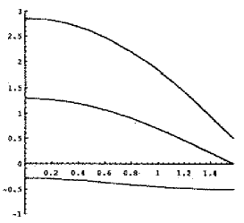
Figure 1: The magnitude of the vacuum polarization $4\pi\langle\varphi^{2}\rangle(\rho)/\sqrt{\lambda}$ as a function of $\rho$ when the BH mass $M=\pi^{-2}$. The curves correspond to $\alpha=-1,0,1$ as indicated.

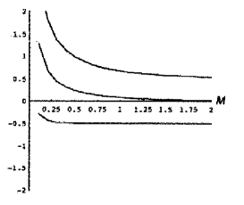
Figure 2: The dependence of the vacuum polarization $4\pi\langle\varphi^{2}\rangle(\rho)/\sqrt{\lambda}$ on the horizon as a function of $M$. The curves correspond to $\alpha=-1,0,1$ as indicated.

The value of $4\pi\langle\varphi^{2}\rangle(\rho)/\sqrt{\lambda}$ is plotted in Fig. 1 for $\alpha=-1,0$, and $1$ when the BH mass $M=\pi^{-2}$. The dependence of $\langle\varphi^{2}\rangle$ at the horizon ($\rho=0;r=r_{H}$) on the BH mass $M$ is shown in Fig. 2. The value of $\langle\varphi^{2}\rangle$ at the horizon approaches a constant $-\alpha\sqrt{\lambda}/(8\pi)$ in the large mass limit.

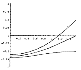
Figure 3: The magnitude of the vacuum polarization $4\pi\langle\varphi^{2}\rangle_{twisted}(\rho)/\sqrt{\lambda}$ as a function of $\rho$ when the BH mass $M=\pi^{-2}$. The curves correspond to $\alpha=-1,0,1$ as indicated.

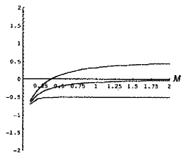
Figure 4: The dependence of the vacuum polarization $4\pi\langle\varphi^{2}\rangle_{twisted}(\rho)/\sqrt{\lambda}$ on the horizon as a function of $M$. The curves correspond to $\alpha=-1,0,1$ as indicated.

For the twisted scaIar field, we obtain

$$\langle\varphi^{2}\rangle_{twisted}(\rho)=-\alpha\frac{\sqrt{\lambda}}{8\pi}$$

$$+\sum_{k=1}^{\infty}(-1)^{k}\left[\frac{\sqrt{\lambda}\cos\rho}{2\sqrt{2}\pi\sqrt{\cosh 2\pi\sqrt{M}k-1}}-\alpha\frac{\sqrt{\lambda}\cos\rho}{2\sqrt{2}\pi\sqrt{\cosh 2\pi\sqrt{M}k+\cos 2\rho}}\right]\,.$$ (16)

The figures corresponding to Figs. 1 and 2 are exhibited as Figs. 3 and 4 for the twisted scalar field.

Now we turn to the vacuum stress tensor. From (13) and (14), we find the simple form

$$\langle T^{\mu}_{\nu}\rangle(\rho)=F(\rho)\mbox{diag}(1,1,-2)+H(\rho)\mbox{diag}(1,0,-1)\,,$$ (17)

where

$$F(\rho)=\frac{\lambda^{3/2}\cos^{3}\rho}{16\sqrt{2}\pi}\sum_{K=1}^{\infty}\left[\frac{1}{(\cosh 2\pi\sqrt{M}k-1)^{1/2}}+\frac{4}{(\cosh 2\pi\sqrt{M}k-1)^{3/2}}\right.$$

$$\left.-\alpha\frac{\cosh 2\pi\sqrt{M}k-1}{(\cosh 2\pi\sqrt{M}k+\cos 2\rho)^{3/2}}\right]\,,$$ (18)

$$H(\rho)=-\alpha\frac{3\lambda^{3/2}\sin^{2}\rho\cos^{3}\rho}{8\sqrt{2}\pi}\sum_{K=1}^{\infty}\frac{\cosh 2\pi\sqrt{M}k-1}{(\cosh 2\pi\sqrt{M}k+\cos 2\rho)^{5/2}}\,.$$ (19)

Obviously the vacuum stress tensor is traceless. One can also check the conservation law $\nabla_{\mu}\langle T^{\mu}_{\nu}\rangle=0$ in the 3DBH background.

For the twisted scalar, we have

$$\langle T^{\mu}_{\nu}\rangle_{twisted}(\rho)=F_{twisted}(\rho)\mbox{diag}(1,1,-2)+H_{twisted}(\rho)\mbox{diag}(1,0,-1)\,,$$ (20)

with

$$F_{twisted}(\rho)=\frac{\lambda^{3/2}\cos^{3}\rho}{16\sqrt{2}\pi}\sum_{K=1}^{\infty}\left[\frac{(-1)^{k}}{(\cosh 2\pi\sqrt{M}k-1)^{1/2}}+\frac{4(-1)^{k}}{(\cosh 2\pi\sqrt{M}k-1)^{3/2}}\right.$$

$$\left.-\alpha\frac{(-1)^{k}(\cosh 2\pi\sqrt{M}k-1)}{(\cosh 2\pi\sqrt{M}k+\cos 2\rho)^{3/2}}\right]\,,$$ (21)

$$H_{twisted}(\rho)=-\alpha\frac{3\lambda^{3/2}\sin^{2}\rho\cos^{3}\rho}{8\sqrt{2}\pi}\sum_{K=1}^{\infty}\frac{(-1)^{k}(\cosh 2\pi\sqrt{M}k-1)}{(\cosh 2\pi\sqrt{M}k+\cos 2\rho)^{5/2}}\,.$$ (22)

The translation to the stress tensor in terms of the coordinate $(t,r,\theta)$ is trivially performed. In the next section, we will mainly use the original coordinate system like (3).

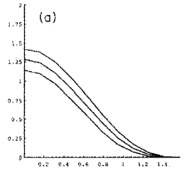
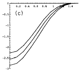
Figure 5: The magnitude of the vacuum polarization $16\pi\langle T^{\mu}_{\nu}\rangle(\rho)/\lambda^{3/2}$ as a function of $\rho$ when the BH mass $M=\pi^{-2}$. Three diagonal components are shown in separate figures: (a) $(\mu,\nu)=(t,t)$, (b) $(\mu,\nu)=(r,r)$, and (c) $(\mu,\nu)=(\theta,\theta)$. The curves correspond to $\alpha=-1,0,1$ as indicated.

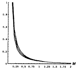
Figure 6: The dependence of the vacuum polarization $16\pi\langle T^{\mu}_{\nu}\rangle(\rho)/\lambda^{3/2}$ on the horizon as a function of $M$. The curves correspond to $\alpha=-1,0,1$ as indicated.

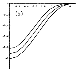
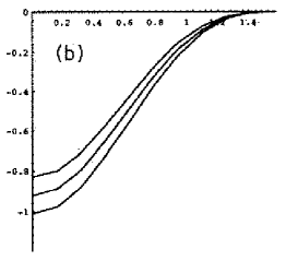
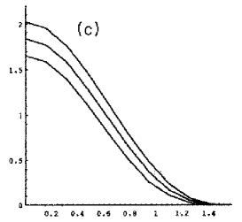
Figure 7: The magnitude of the vacuum polarization $16\pi\langle T^{\mu}_{\nu}\rangle_{twisted}(\rho)/\lambda^{3/2}$ as a function of $\rho$ when the BH mass $M=\pi^{-2}$. Three diagonal components are shown in separate figures: (a) for $(\mu,\nu)=(t,t)$, (b) $(\mu,\nu)=(r,r)$, and (c) $(\mu,\nu)=(\theta,\theta)$. The curves correspond to $\alpha=-1,0,1$ as indicated.

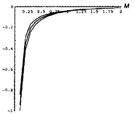
Figure 8: The dependence of the vacuum polarization $16\pi\langle T^{\mu}_{\nu}\rangle_{twisted}(\rho)/\lambda^{3/2}$ on the horizon as a function of $M$. The curves correspond to $\alpha=-1,0,1$ as indicated.

The numerical results for the vacuum stress energy is shown in Figs. 5–8. The value of $16\pi\langle T^{\mu}_{\nu}\rangle(\rho)/\lambda^{3/2}$ is plotted in Fig. 5 for $\alpha=-1,0$, and $1$ when the BH mass $M=\pi^{-2}$.

The dependence of $\langle T^{\mu}_{\nu}\rangle$ at the horizon $(\rho=0;r=r_{H})$ on the BH mass $M$ is shown in Fig. 6. The values of $\langle T^{\mu}_{\nu}\rangle$ at the horizon approaches zero in the large mass limit. On the other hand, in the limit of $M\rightarrow 0$, all components of $\langle T^{\mu}_{\nu}\rangle$ diverge. Note also that $\langle T^{t}_{t}\rangle=\langle T^{r}_{r}\rangle$ is satisfied on the horizon.

In the limit of $\rho=\pi/2$ ($r\rightarrow\infty$), all the components of $\langle T^{\mu}_{\nu}\rangle$ for any case become zero. One can regard that this is due to the “redshift” factor $(|g_{tt}|)^{-1/2}$ which goes to zero at spatial infinity. Thus, thermal equilibrium is not attained between the BH and the radiation in this system. For the twisted scalar field, $16\pi\langle T^{\mu}_{\nu}\rangle_{twisted}(\rho)/\lambda^{3/2}$ is exhibited in the same format as the untwisted case in Figs. 7 and 8. It turns out that the value of $\langle T^{\mu}_{\nu}\rangle$ is not so sensitive to the value of $\alpha$ for all cases. In the subsequent section, we consider back reaction of the quantum effect to the metric.

4 BACK REACTION TO THE SPACE-TIME METRIC

In this section, we investigate the effect of back reaction due to the quantum effects. The back reaction of quantum fields to the metric has been studied in the Schwarzschild metric in four dimensions [15, 16, 17, 18]. We will examine the correction to the gravitational force on test particles using the corrected metric.

The vacuum values obtained in the preceding section are quantities of $O(h)$, or one-loop quantum corrections. The Einstein equation is modified by the vacuum stress tensor and then becomes

$$R^{\mu}_{\nu}-\frac{1}{2}R\delta^{\mu}_{\nu}-\lambda\delta^{\mu}_{\nu}=\pi\langle T^{\mu}_{\nu}\rangle\,.$$ (23)

We choose the small parameter which denotes the perturbation. The perturbation parameter, $\varepsilon$, should be proportional to the Planck constant, which is set by unity here. Hence we will take $\varepsilon=1/r_{H}$, since the Planck length is proportional to h in three dimensions.

Consequently, we need only the expression of the vacuum stress tensor in the large mass limit. We have for $\alpha\neq 1$,

$$\langle T^{\mu}_{\nu}\rangle_{\pm}=\pm\frac{(\sqrt{\lambda}r_{H})^{3}}{16\pi r^{3}}(1-\alpha)e^{-\pi\sqrt{M}}\mbox{diag}(1,1,-2)+O(e^{-3\pi\sqrt{M}})\quad(\alpha\neq 1)$$ (24)

and for $\alpha=1$,

$$\langle T^{\mu}_{\nu}\rangle_{\pm}=\pm\frac{(\sqrt{\lambda}r_{H})^{3}}{8\pi r^{3}}e^{-3\pi\sqrt{M}}\mbox{diag}\left(\frac{9r_{H}^{2}}{r^{2}}-1,\frac{3r_{H}^{2}}{r^{2}}+4,-\frac{12r_{H}^{2}}{r^{2}}-2\right)$$

$$\qquad\qquad+O(e^{-5\pi\sqrt{M}})\quad(\alpha=1)\,,$$ (25)

where $\langle T^{\mu}_{\nu}\rangle_{+}$ represents $\langle T^{\mu}_{\nu}\rangle$ for the untwisted scalar and $\langle T^{\mu}_{\nu}\rangle_{-}$ represents $\langle T^{\mu}_{\nu}\rangle_{twisted}$ for the twisted scalar and the signs on the right-hand side correspond to them respectively.

We use their leading terms in the analysis in this section. Of course, they are traceless and covariantly conserved.

We consider the following metric which suffers the quantum effect:

$$ds^{2}=-e^{2\psi(r)}[\lambda r^{2}-m(r)]dt^{2}+\frac{dr^{2}}{\lambda r^{2}-m(r)}+r^{2}d\theta^{2}$$ (26)

where $m(r)$ and $\psi(r)$ is the function of $r$ which are to be solved to satisfy the Einstein equations with quantum correction.

Using the metric (26), the $(t,t)$ component of the Einstein equation (23 reads

$$-\frac{1}{2r}\frac{dm(r)}{dr}=\pi\langle T^{t}_{t}\rangle\,,$$ (27)

and similarly a linear combination of the $(t,t)$ and $(r,r)$ components of the Einstein equation leads to

$$-\frac{\lambda r^{2}-m(r)}{r}\frac{d\psi(r)}{dr}=\pi(\langle T^{t}_{t}\rangle-\langle T^{r}_{r}\rangle)\,.$$ (28)

Equation (27) is solved in the form

$$m(r)=M[1+\varepsilon\mu(r)]\,,$$ (29)

with

$$\mu(r)=-\frac{2\pi r_{H}}{M}\int_{r_{H}}^{r}\langle T^{t}_{t}\rangle\bar{r}d\bar{r}\,,$$ (30)

where the mass of the BH is “renormalized” so that $m(r_{H})=M$ [15, 16, 17].

Similarly, Eq. (28) can be solved to the first-order perturbation in the form

$$\psi(r)=\varepsilon[\rho(r)-\rho(r_{0})]\,,$$ (31)

with

$$\rho(r)=-\pi r_{H}\int_{r_{H}}^{r}\frac{\langle T^{t}_{t}\rangle-\langle T^{r}_{r}\rangle}{\lambda\bar{r}^{2}-M}\bar{r}d\bar{r}\,,$$ (32)

where we assume the boundary condition $\psi(r_{0})=0$ [15, 16, 17].

We treat two cases for $\alpha\neq 1$ and for $\alpha=1$ separately.

(1) For $\alpha\neq 1$. We use the leading contribution in (24). Then Eq. (28) is solved as $\psi=0$, and we get

$$\mu_{\pm}(r)=\pm\frac{(1-\alpha)(\sqrt{\lambda}r_{H})^{3}}{8M}e^{-\pi\sqrt{M}}\left(\frac{r_{H}}{r}-1\right)\quad(\alpha\neq 1)\,,$$ (33)

Here the plus (minus) sign corresponds to the case with the untwisted (twisted) scalar field.

(2) For $\alpha=1$. The correction to the BH mass is given, for a large value of $M$, by

$$\mu_{\pm}(r)=\pm\frac{(\sqrt{\lambda}r_{H})^{3}}{4M}e^{-3\pi\sqrt{M}}\left[3\left(\frac{r_{H}}{r}\right)^{3}-2\frac{r_{H}}{r}-1\right]\quad(\alpha=1)\,,$$ (34)

while substitution of (25) into (32) gives

$$\rho_{\pm}(r)=\pm\frac{(\sqrt{\lambda}r_{H})^{3}}{4M}e^{-3\pi\sqrt{M}}\left[1-\left(\frac{r_{H}}{r}\right)^{3}\right]\quad(\alpha=1)\,.$$ (35)

The mass correction $\mu$ take a finite value in the large-$r$ limit in each case. That is

$$m_{\pm}(\infty) = M\mp\varepsilon\frac{(1-\alpha)M^{3/2}}{8}e^{-\pi\sqrt{M}}\quad(\alpha\neq 1)\,,$$ (36)

$$m_{\pm}(\infty) = M\mp\varepsilon\frac{M^{3/2}}{4}e^{-3\pi\sqrt{M}}\qquad\qquad(\alpha=1)\,,$$ (37)

where we leave the parameter $\varepsilon$ which manifestly displays the perturbation. For the untwisted scalar field, the mass correction is negative (positive) for $\alpha\leq 1$ ($\alpha>1$) in the asymptotic region. For the twisted scalar field, the sign is reversed.

Now let us examine the property of the corrected geometry using the results obtained above. The magnitude of the static gravitational force on a test particle placed in the BH geometry is indicated by the “radial acceleration in the proper rest frame of the particle” defined by [16]

$$a=\frac{1}{2}\sqrt{g^{rr}}\frac{\partial}{\partial r}\ln|g_{tt}|\,.$$ (38)

The positive value for a means the attractive force.

In this expression, we will use the corrected metric up to the first order in c; the relevant components are

$$g^{rr}(A\lambda r^{2}-M)\left[1-\varepsilon\frac{M}{\lambda r^{2}-M}\mu(r)\right]$$ (39)

and

$$|g_{tt}|(r)=(\lambda r^{2}-M)\left\{1+\varepsilon\left[2[\rho(r)-\rho(r_{0})]-\frac{M}{\lambda r^{2}-M}\mu(r)\right]\right\}\,.$$ (40)

Inserting these components into (38), we obtain

$$a=\frac{\lambda r}{\sqrt{\lambda r^{2}-M}}\{1+\varepsilon\Delta(r)\}\,,$$ (41)

where the correction term is given by

$$\Delta(r)=\frac{M}{2(\lambda r^{2}-M)}\mu(r)+\frac{\pi\sqrt{M}}{\lambda^{3/2}}\langle T^{r}_{r}\rangle(r)\,.$$ (42)

We calculate this using the previous results for the quantum effect of a conformally invariant scalar field. For $a\neq 1$, the correction is written in the form

$$\Delta_{\pm}(r)=\pm(1-\alpha)\frac{\sqrt{M}}{16}e^{-\pi\sqrt{M}}\frac{\cos^{2}\rho+\cos\rho-1}{1+\cos\rho}\cos^{3}\rho\quad(\alpha\neq 1)\,,$$ (43)

while for $\alpha=1$,

$$\Delta_{\pm}(r)=\pm\frac{\sqrt{M}}{8}e^{-\pi\sqrt{M}}\frac{3\cos^{3}\rho+4\cos^{2}\rho+\cos\rho-1}{1+\cos\rho}\cos^{2}\rho\quad(\alpha=1)\,,$$ (44)

where $\cos\rho=r_{H}/r$.

We find that, for the untwisted scalar field and $\alpha\leq 1$, the quantum correction gives positive contribution in a certain region $r<r_{c}$, and negative contribution in the outside region. Namely, the quantum effect diminishes the attractive force in the region $r>r_{c}$.

The value for $r_{c}$ is given by

$$r_{c}\simeq 1.618r_{H}\quad\mbox{for }\alpha\neq 1\,,$$ (45)

$$r_{c}\simeq 2.806r_{H}\quad\mbox{for }\alpha=1\,.$$ (46)

For the twisted field or for $\alpha>$1, the sign of the correction $\Delta$ is reversed.

The correction force is negligibly small for large $M$ and vanishes at spatial infinity. Therefore, the quantum correction due to the conformal scalar field cannot be comparable to the classical attractive force.

5 DISCUSSION

In this paper, we have obtained the propagator for a conformally coupled massless scalar field in 3DBH space-time with Euclidean signature. Using the exact propagator, we have computed the vacuum expectation value $\langle\varphi^{2}\rangle$ and stress tensor for untwisted and twisted scalar fields.

The back reaction to the metric has also been discussed in the present paper. The quantum correction to the gravitational force on the static test particle has been estimated. It is found that there are a critical radius outside the BH, which divides the regions where the positive and negative correction arise.

For large values of the BH mass, the quantum effects become exponentially small. One may expect that the back reaction becomes important only if the BH is small, or, at the final stage of the BH evaporation. In such cases, the perturbative analysis is no longer valid.

One may wish to study the thermodynamics of the 3DBH including the quantum field back reaction. Such analyses have been carried out in Ref. [17] for four-dimensional BH’s. The approach used in Ref. [17] is equally effective for the three-dimensional case. However, there exist some subtleties in the 3DBH case which arise from the existence of the additional length scale $\lambda^{-1/2}$ and the $h$ independence of the Planck mass in three dimensions. We leave the discussion on the thermodynamics with quantum fields for separate publications.

In the present paper, we discussed only conformal massless scalar field. The other types of the fields should be taken into the general analysis.

The quantum-field theory around a rotating 3DBH is an interesting subject worth studying. The thermodynamics of the rotating 3DBH’s including quantum fields should be clearly understood in the future.

Note added. After completion of this manuscript, we became aware of the works by Steif [19] and by Lifshifts and Ortiz [20]. Steif calculated the stress tensor $\langle T^{\mu}_{\nu}\rangle$ for the scalar field with transparent boundary condition ($\alpha=0$ in our case). He also studied the rotating BH background. Lifschytz and Ortiz considered the Dirichlet and Neumann boundary conditions ($\alpha=1$ and $-1$ in our case, respectively). They also calculated a response function for a scalar field outside the BH horizon.

References

[1]Quantum Theory of Gravity, edited by S. M.
Christensen (Hilger, Bristol, 1984); Conceptual Problems of
Quantum gravity, edited by A. Ashtekar and J. Stachel (Birkhauser,
Boston, 1991); E. Alvarez, Rev. Mod. Phys. 61 (1989) 561.
[2] N. D. Birrell and P. C. W. Davies, Quantum Fields in
Curved Space (Cambridge University Press, Cambridge,
England, 1982).
[3] P. Candelas, Phys. Rev. D21 (1980) 2185; P. Candelas
and K. W. Howard, ibid. D29 (1984) 1618; K. W. Howard
and P. Candelas, Phys. Rev. Lett. 53 (1984) 403; K. W.
Howard, Phys. Rev. D30 (1984) 2532; V. P. Frolov, ibid.
D26 (1982) 954; V. P. Frolov, F. D. Mazzitelli and J. P.
Paz, ibid. D40 (1990) 948; I. D. Novikov and V. P. Frolov,
Physics of Black Holes (Kluwer Academic, Dordrecht,
1988); V. P. Frolov, in Trends in Theoretical Physics, edited
by P. J. Ellis and Y. C. Tang (Addison-Wesley, Reading,
MA, 1991), Vol. 2, pp. 27–75; P. R. Anderson, Phys.
Rev. D39 (1989) 3785; D41 (1990) 1152.
[4] M. Banados, C. Teitelboim and J. Zanelli, Phys. Rev.
Lett. 69 (1992) 1849; M. Bandados, M. Henneaux, C.
Teitelboim and J. Zanelli, Phys. Rev. D48 (1993) 1506.
[5] S. F. Ross aud R. B. Mann, Phys. Rev. D47 (1993)
3319; D. Cangemi, M. Leblanc and R. B. Mann, ibid. D48 (1993)
3606; A. Achucarro and M. Ortiz, ibid. D48 (1993) 3600; G. T.
Horowitz and D. L. Welch, Phys. Rev. Lett. 71 (1993) 328; N.
Kaloper, Phys. Rev. D48 (1993) 2598; C. Farina, J. Gamboa and A.
J. Segui-Santonja, Class. Quantum Grav. 10 (1993) L193.
[6] K. Shiraishi and T. Maki, Class. Quantum Grav.
11 (1994) 695.
[7] C. W. Misner, K. S. Thorne and J. A. Wheeler,
Gravitation (Freeman, San Francisco, 1973).
[8] S. J. Avis, C. J. Isham and D. Storey, Phys. Rev. D18
(1978) 3565.
[9] C. P. Burgess and C. A. Lutken, Phys. Lett. B153
(1985) 137.
[10] C. J. C. Burges et al., Ann. Phys. (N.Y.) 167 (1986)
285.
[11] B. Allen, A. Folacci and G. W. Gibbons, Phys. Lett.
B189 (1987) 304.
[12] A. G. Smith, in The Formation and Evolution of
Cosmic Strings, edited by G. W. Gibbons, S. W. Hawking, and T.
Vachaspati (Cambridge University Press, Cambridge,
England, 1990).
[13] For an example, V. P. Frolov, C. M. Massacand and C.
Schmid, Phys. Lett. B279 (1992) 29.
[14] C. J. Isham, Proc. R. Soc. London A362 (1978) 383;
A364 (1978) 591; L. H. Ford, Phys. Rev. D21 (1980) 949.
[15] J. W. York, Phys. Rev. D31 (1985) 775.
[16] D. Hochberg and T. W. Kephart, Phys. Rev. D47 (1993)
1465; D. Hochberg, T. W. Kephart and J. W. York, Phys. Rev. D49
(1994) 5257.
[17] D. Hochberg, T. W. Kephart aud J. W. York, Phys. Rev.
D48 (1993) 479.
[18] J. W. York, Phys. Rev. D33 (1986) 2092.
[19] A. Steif, Phys. Rev. D49 (1994) 585.
[20] G. Lifschytz aud M. Ortiz, Phys. Rev. D49 (1994)
1929.