Mutual Information Maximization for Simple and Accurate Part-Of-Speech Induction

Abstract

We address part-of-speech (POS) induction by maximizing the mutual information between the induced label and its context. We focus on two training objectives that are amenable to stochastic gradient descent (SGD): a novel generalization of the classical Brown clustering objective and a recently proposed variational lower bound. While both objectives are subject to noise in gradient updates, we show through analysis and experiments that the variational lower bound is robust whereas the generalized Brown objective is vulnerable. We obtain strong performance on a multitude of datasets and languages with a simple architecture that encodes morphology and context.

1 Introduction

We consider information theoretic objectives for POS induction, an important unsupervised learning problem in computational linguistics Christodoulopoulos et al. (2010). The idea is to make the induced label syntactically informative by maximizing its mutual information with respect to local context. Mutual information has long been a workhorse in the development of NLP techniques, for instance the classical Brown clustering algorithm Brown et al. (1992). But its role in today’s deep learning paradigm is less clear and a subject of active investigation (Belghazi et al., 2018; Oord et al., 2018).

We focus on fully differentiable objectives that can be plugged into an automatic differentiation system and efficiently optimized by SGD. Specifically, we investigate two training objectives. The first is a novel generalization of the Brown clustering objective obtained by relaxing the hard clustering constraint. The second is a recently proposed variational lower bound on mutual information (McAllester, 2018).

A main challenge in optimizing these objectives is the difficulty of stochastic optimization. Each objective involves entropy estimation which is a nonlinear function of all data and does not decompose over individual instances. This makes the gradients estimated on minibatches inconsistent with the true gradient estimated from the entire dataset. To our surprise, in practice we are able to optimize the variational objective effectively but not the generalized Brown objective. We analyze the estimated gradients and show that the inconsistency error is only logarithmic in the former but linear in the latter.

We validate our approach on POS induction by attaining strong performance on a multitude of datasets and languages. Our simple architecture that encodes morphology and context reaches up to 80.1 many-to-one accuracy on the 45-tag Penn WSJ dataset and achieves 4.7% absolute improvement to the previous best result on the universal treebank. Unlike previous works, our model does not rely on computationally expensive structured inference or hand-crafted features.

2 Background

2.1 Information Theory

Mutual information.

Mutual information between two random variables measures the amount of information gained about one variable by observing the other. Unlike the Pearson correlation coefficient which only captures the degree of linear relationship, mutual information captures any nonlinear statistical dependencies (Kinney and Atwal, 2014).

Formally, the mutual information between discrete random variables $X,Y$ with a joint distribution $p$ is the KL divergence between the joint distribution $p(x,y)$ and the product distribution $p(x)p(y)$ over $X,Y$:

$$I(X,Y) =\sum_{x,y}p(x,y)\log\frac{p(x,y)}{p(x)p(y)}$$

$$=\underset{(x,y)\sim p}{\textbf{E}}\left[\log\frac{p(x,y)}{p(x)p(y)}\right]$$ (1)

It is thus nonnegative and zero iff $X$ and $Y$ are independent. We assume that the marginals $p(x)$ and $p(y)$ are nonzero.

It is insightful to write mutual information in terms of entropy. The entropy of $X$ is

$$H(X)=-\sum_{x}p(x)\log p(x)=\underset{x\sim p}{\textbf{E}}\left[\log\frac{1}{p(x)}\right]$$

corresponding to the number of bits for encoding the behavior of $X$ under $p$. The entropy of $X$ given the information that $Y$ equals $y$ is

$$H(X|Y=y)=-\sum_{x}p(x|y)\log p(x|y)$$

Taking expectation over $Y$ yields the conditional entropy of $X$ given $Y$:

$$H(X|Y) =\sum_{y}p(y)\left(-\sum_{x}p(x|y)\log p(x|y)\right)$$

$$=\underset{(x,y)\sim p}{\textbf{E}}\left[\log\frac{1}{p(x|y)}\right]$$ (2)

By manipulating the terms in mutual information, we can write

$$I(X,Y) =\underset{x\sim p}{\textbf{E}}\left[\log\frac{1}{p(x)}\right]-\underset{(x,y)\sim p}{\textbf{E}}\left[\log\frac{1}{p(x|y)}\right]$$

$$=H(X)-H(X|Y)$$

which expresses the amount of information on $X$ gained by observing $Y$. Switching $X$ and $Y$ shows that $I(X,Y)=H(Y)-H(Y|X)$.

Cross entropy.

If $p$ and $q$ are full-support distributions over the same discrete set, the cross entropy between $p$ and $q$ is the asymmetric quantity

$$H(p,q)=-\sum_{x}p(x)\log q(x)=\underset{x\sim p}{\textbf{E}}\left[\log\frac{1}{q(x)}\right]$$

corresponding to the number of bits for encoding the behavior of $X$ under $p$ by using $q$. It is revealing to write entropy in terms of KL divergence. Multiplying the term inside the log by $p(x)/p(x)$ we derive

$$H(p,q) =\underset{x\sim p}{\textbf{E}}\left[\log\frac{1}{p(x)}\right]+\underset{x\sim p}{\textbf{E}}\left[\log\frac{p(x)}{q(x)}\right]$$

$$=H(p)+D_{\mathrm{KL}}(p||q)$$

Thus $H(p,q)\geq H(p)$ with equality iff $p=q$.

2.2 Brown Clustering

Our primary inspiration comes from Brown clustering (Brown et al., 1992), a celebrated word clustering technique that had been greatly influential in unsupervised and semi-supervised NLP long before continuous representations based on neural networks were popularized. It finds a clustering $C:V\rightarrow[m]$ of the vocabulary $V$ into $m$ classes by optimizing the mutual information between the clusters of a random bigram $(X,Y)$. Given a corpus of $N$ words $(x_{1}\ldots x_{N})$, it assumes a uniform distribution over consecutive word pairs $(x_{i-1},x_{i})$ and optimizes the following empirical objective

$$\max_{C:V\rightarrow[m]}\sum_{c,c^{\prime}\in[m]}\frac{\#(c,c^{\prime})}{N}\log\left(\frac{\#(c,c^{\prime})N}{\#(c)\#(c^{\prime})}\right)$$ (3)

where $\#(c,c^{\prime})$ denotes the number of occurrences of the cluster pair $(c,c^{\prime})$ under $C$. While this optimization is intractable, Brown et al. (1992) derive an effective heuristic that 1. initializes $m$ most frequent words as singleton clusters and 2. repeatedly merges a pair of clusters that yields the smallest decrease in mutual information. The resulting clusters have been useful in many applications (Koo et al., 2008; Owoputi et al., 2013) and has remained a strong baseline for POS induction decades later Christodoulopoulos et al. (2010). But the approach is tied to highly nontrivial combinatorial optimization tailored for the specific problem and difficult to scale/generalize.

3 Objectives

In the remainder of the paper, we assume discrete random variables $(X,Y)\in\mathcal{X}\times\mathcal{Y}$ with a joint distribution $D$ that represent naturally co-occurring observations. In POS induction experiments, we will set $D$ to be a context-word distribution where $Y$ is a random word and $X$ is the surrounding context of $Y$ (thus $\mathcal{Y}$ is the vocabulary and $\mathcal{X}$ is the space of all possible contexts). Let $m$ be the number of labels to induce. We introduce a pair of trainable classifiers that define conditional label distributions $p(z|x)$ and $q(z|y)$ for all $x\in\mathcal{X}$, $y\in\mathcal{Y}$, and $z\in[m]$. For instance, $p(\cdot|y)$ can be the output of a softmax layer on some transformation of $y$.

Our goal is to learn these classifiers without observing the latent variable $z$ by optimizing an appropriate objective. For training data, we assume $N$ iid samples $(x_{1},y_{1})\ldots(x_{N},y_{N})\sim D$.

3.1 Generalized Brown Objective

Our first attempt is to maximize the mutual information between the predictions of $p$ and $q$. Intuitively, this encourages $p$ and $q$ to agree on some annotation scheme (up to a permutation of labels), modeling the dynamics of inter-annotator agreement Artstein (2017). It can be seen as a differentiable generalization of the Brown clustering objective. To this end, define

$$p(z) =\underset{x\sim D}{\textbf{E}}\left[p(z|x)\right] \forall z\in[m]$$

$$q(z) =\underset{y\sim D}{\textbf{E}}\left[q(z|y)\right] \forall z\in[m]$$

The mutual information between the predictions of $p$ and $q$ on a single sample $(x,y)$ is then

$$J^{\mathrm{mi}}_{x,y}=\sum_{z,z^{\prime}}p(z|x)q(z^{\prime}|y)\log\frac{p(z|x)q(z^{\prime}|y)}{p(z)q(z^{\prime})}$$

and the objective (to maximize) is

$$J^{\mathrm{mi}}=\underset{(x,y)\sim D}{\textbf{E}}\left[J^{\mathrm{mi}}_{x,y}\right]$$

Note that this becomes exactly the original Brown objective (3) if $(X,Y)$ is defined as a random bigram and $p$ and $q$ are tied and constrained to be a hard clustering.

Empirical objective.

In practice, we work with the value of empirical mutual information $\widehat{J}^{\mathrm{mi}}$ estimated from the training data:

$$\hat{p}(z) =\frac{1}{N}\sum_{i=1}^{N}p(z|x_{i})\hskip 56.9055pt\forall z\in[m]$$

$$\hat{q}(z) =\frac{1}{N}\sum_{i=1}^{N}q(z|y_{i})\hskip 59.75078pt\forall z\in[m]$$

$$\widehat{J}^{\mathrm{mi}}_{i} =\sum_{z,z^{\prime}}p(z|x_{i})q(z^{\prime}|y_{i})\log\frac{p(z|x_{i})q(z^{\prime}|y_{i})}{\hat{p}(z)\hat{q}(z^{\prime})}$$

$$\widehat{J}^{\mathrm{mi}} =\frac{1}{N}\sum_{i=1}^{N}\widehat{J}^{\mathrm{mi}}_{i}$$ (4)

Our task is to maximize (4) by taking gradient steps at random minibatches. Note, however, that the objective cannot be written as a sum of local objectives because we take log of the estimates $\hat{q}(z)$ and $\hat{p}(z)$ computed from all samples. This makes the stochastic gradient estimator biased (i.e., it does not match the gradient of (4) in expectation) and compromises the correctness of SGD. This bias is investigated more closely in Section 4.

3.2 Variational Lower Bound

The second training objective we consider can be derived in a rather heuristic but helpful manner as follows. Since $X,Y$ are always drawn together, if $q(z|y)$ is the target label distribution for the pair $(x,y)$, then we can train $p(z|x)$ by minimizing the cross entropy between $q$ and $p$ over samples

$$H(q,p) =\underset{(x,y)\sim D}{\textbf{E}}\left[-\sum_{z}q(z|y)\log p(z|x)\right]$$

which is minimized to zero at $p=q$. However, $q$ is also untrained and needs to be trained along with $p$. Thus this loss alone admits trivial solutions such as setting $p(1|x)=p(1|y)=1$ for all $(x,y)$. This undesirable behavior can be prevented by simultaneously maximizing the entropy of $q$. Let $Z$ denote a random label from $q$ with distribution $q(z)=\underset{y\sim D}{\textbf{E}}\left[q(z|y)\right]$ (thus $Z$ is a function of $q$). The entropy of $Z$ is

$$H(Z) =-\sum_{z}q(z)\log q(z)$$

Putting together, the objective (to maximize) is

$$J^{\mathrm{var}}=H(Z)-H(q,p)$$

Variational interpretation.

The reason this objective is named a variational lower bound is due to McAllester (2018) who shows the following. Consider the mutual information between $Z$ and the raw signal $X$:

$$I(X,Z)=H(Z)-H(Z|X)$$ (5)

Because $Z$ is drawn from $q$ conditioning on $Y$, which is co-distributed with $X$, we have a Markov chain $X\rightarrow Y\xrightarrow{q}Z$. Thus maximizing $I(X,Z)$ over the choice of $q$ is a reasonable objective that enforces “predictive coding”: the label predicted by $q$ from $Y$ must be as informative of $X$ as possible. It can be seen as a special case of the objective underlying the information bottleneck method (Tishby et al., 2000).

So what is the problem with optimizing (5) directly? The problem is that the conditional entropy under the model

$$H(Z|X)=\underset{\begin{subarray}{c}(x,y)\sim D\\ z\sim q(\cdot|y)\end{subarray}}{\textbf{E}}\left[\log\frac{1}{\pi(z|x)}\right]$$ (6)

involves the posterior probability of $z$ given $x$

$$\pi\left(z|x\right)=\frac{\sum_{y}D(x,y)q(z|y)}{\sum_{y,z}D(x,y)q(z|y)}$$

This conditional marginalization is generally intractable and cannot be approximated by sampling since the chance of seeing a particular $x$ is small. However, we can introduce a variational distribution $p(z|x)$ to model $\pi\left(z|x\right)$. Plugging this into (6) we observe that

$$\underset{\begin{subarray}{c}(x,y)\sim D\\ z\sim q(\cdot|y)\end{subarray}}{\textbf{E}}\left[\log\frac{1}{p(z|x)}\right]=H(q,p)$$

Moreover,

$$\underset{\begin{subarray}{c}(x,y)\sim D\\ z\sim q(\cdot|y)\end{subarray}}{\textbf{E}}\left[\log\frac{1}{p(z|x)}\right]$$

$$\hskip 28.45274pt=\underset{\begin{subarray}{c}(x,y)\sim D\\ z\sim q(\cdot|y)\end{subarray}}{\textbf{E}}\left[\log\frac{\pi\left(z|x\right)}{\pi\left(z|x\right)p(z|x)}\right]$$

$$\hskip 28.45274pt=H(Z|X)+D_{\mathrm{KL}}(\pi||p)$$

Thus $H(q,p)$ is an upper bound on $H(Z|X)$ for any $p$ with equality iff $p$ matches the true posterior distribution $\pi$. This in turn means that $J^{\mathrm{var}}=H(Z)-H(q,p)$ is a lower bound on $I(X,Z)$, hence the name.

Empirical objective.

As with the generalized Brown objective, the variational lower bound can be estimated from the training data as

$$\widehat{H}(Z) =-\sum_{z}\hat{q}(z)\log\hat{q}(z)$$

$$\widehat{H}(q,p) =\frac{1}{N}\sum_{i=1}^{N}\left(-\sum_{z}q(z|y_{i})\log p(z|x_{i})\right)$$

$$\widehat{J}^{\mathrm{var}} =\widehat{H}(Z)-\widehat{H}(q,p)$$ (7)

where $\hat{q}(z)$ is defined as in Section 3.1. Our task is again to maximize this empirical objective (7) by taking gradient steps at random minibatches. Once again, it cannot be written as a sum of local objectives because the entropy term involves log of $\hat{q}(z)$ computed from all samples. Thus it is not clear if stochastic optimization will be effective.

4 Analysis

The discussion of the two objectives in the previous section is incomplete because the stochastic gradient estimator is biased under both objectives. In this section, we formalize this issue and analyze the bias.

4.1 Setting

Let $B_{1}\ldots B_{K}$ be a partition of the $N$ training examples $(x_{1},y_{1})\ldots(x_{N},y_{N})$ into $K$ (iid) minibatches. For simplicity, assume $\left|B_{k}\right|=M$ for all $k$ and $N=MK$. We will adopt the same notation in Section 3 for $\hat{p}(z)$ and $\hat{q}(z)$ estimated from all $N$ samples. Define analogous estimates based on the $k$-th minibatch by

$$\hat{p}_{k}(z) =\frac{1}{M}\sum_{x\in B_{k}}p(z|x) \forall z\in[m]$$

$$\hat{q}_{k}(z) =\frac{1}{M}\sum_{y\in B_{k}}q(z|y) \forall z\in[m]$$

If $l_{N}$ denotes an objective function computed from all $N$ samples in the training data and $l_{k}$ denotes the same objective computed from $B_{k}$, a condition on the correctness of SGD is that the gradient of $l_{k}$ (with respect to model parameters) is consistent with the gradient of $l_{N}$ on average:

$$\nabla l_{N}=\frac{1}{K}\sum_{k=1}^{K}\nabla l_{k}+\epsilon$$ (8)

where $\epsilon$ denotes the bias of the stochastic gradient estimator. In particular, any loss of the form $l_{N}=(1/K)\sum_{k}l_{k}$ that decomposes over independent minibatches (e.g., the cross-entropy loss for supervised classification) satisfies (8) with $\epsilon=0$. The bias is nonzero for the unsupervised objectives considered in this work due to the issues discussed in Section 3.

4.2 Result

The following theorem precisely quantifies the bias for the empirical losses associated with the variational bound and the generalized Brown objectives. We only show the result with the gradient with respect to $q$, but the result with the gradient with respect to $p$ is analogous and omitted for brevity.

Theorem 4.1.

Assume the setting in Section 4.1 and the gradient is taken with respect to the parameters of $q$. For $l_{N}=-\widehat{J}^{\mathrm{var}}$ defined in (7),

$$\epsilon =\frac{1}{K}\sum_{k=1}^{K}\sum_{z}\log\frac{\hat{q}(z)}{\hat{q}_{k}(z)}\nabla\hat{q}_{k}(z)$$

On the other hand, for $l_{N}=-\widehat{J}^{\mathrm{mi}}$ defined in (4),

$$\epsilon =\frac{1}{N}\sum_{k=1}^{K}\sum_{z,z^{\prime}}\bigg{(}\epsilon_{k}(z,z^{\prime})\nabla\hat{q}_{k}(z^{\prime})$$

$$\hskip 14.22636pt+\log\frac{\hat{p}(z)\hat{q}(z^{\prime})}{\hat{p}_{k}(z)\hat{q}_{k}(z^{\prime})}\sum_{(x,y)\in B_{k}}p(z|x)\nabla q(z^{\prime}|y)\bigg{)}$$

where

$$\epsilon_{k}(z,z^{\prime}) =\frac{1}{K}\sum_{i=1}^{N}\frac{p(z|x_{i})q(z^{\prime}|y_{i})}{\hat{q}(z^{\prime})}$$

$$\hskip 14.22636pt-\sum_{(x,y)\in B_{k}}\frac{p(z|x)q(z^{\prime}|y)}{\hat{q}_{k}(z^{\prime})}$$

A proof can be found in the appendix. We see that both biases go to zero as $\hat{p}_{k}$ and $\hat{q}_{k}$ approach $\hat{p}$ and $\hat{q}$. However, the bias is logarithmic in the ratio $\hat{q}(z)/\hat{q}_{k}(z)$ for the variational lower bound but roughly linear in the difference between $\frac{1}{\hat{q}(z^{\prime})}$ and $\frac{1}{\hat{q}_{k}(z^{\prime})}$ for the generalized Brown objective. In this sense, the variational lower bound is exponentially more robust to noise in minibatch estimates than the generalized Brown objective. This is confirmed in experiments: we are able to optimize $\widehat{J}^{\mathrm{var}}$ with minibatches as small as $80$ examples but unable to optimize $\widehat{J}^{\mathrm{mi}}$ unless minibatches are prohibitively large.

5 Experiments

We demonstrate the effectiveness of our training objectives on the task of POS induction. The goal of this task is to induce the correct POS tag for a given word in context Merialdo (1994). As typical in unsupervised tasks, evaluating the quality of induced labels is challenging; see Christodoulopoulos et al. (2010) for an in-depth discussion. To avoid complications, we follow a standard practice Berg-Kirkpatrick et al. (2010); Ammar et al. (2014); Lin et al. (2015); Stratos et al. (2016) and adopt the following setting for all compared methods.

• We use many-to-one accuracy as a primary evaluation metric. That is, we map each induced label to the most frequently coinciding ground-truth POS tag in the annotated data and report the resulting accuracy. We also use the V-measure (Rosenberg and Hirschberg, 2007) when comparing with CRF autoencoders to be consistent with reported results Ammar et al. (2014); Lin et al. (2015).

• We use the number of ground-truth POS tags as the value of $m$ (i.e., number of labels to induce). This is a data-dependent quantity, for instance 45 in the Penn WSJ and 12 in the universal treebank. Fixing the number of tags this way obviates many evaluation issues.

• Model-specific hyperparameters are tuned on the English Penn WSJ dataset. This configuration is then fixed and used for all other datasets: 10 languages in the universal treebank and 7 languages from CoNLL-X and CoNLL 2007.

5.1 Setting

We set $D$ to be a uniform distribution over context-word pairs in the training corpus. Given $N$ samples $(x_{1},y_{1})\ldots(x_{N},y_{N})\sim D$, we optimize the variational objective (7) or the generalized Brown objective (4) by taking gradient steps at random minibatches. This gives us conditional label distributions $p(z|x)$ and $q(z|y)$ for all contexts $x$, words $y$, and labels $z$. At test time, we use

$$z^{*}=\operatorname*{arg\,max}_{z}q(z|y)$$

as the induced label of word $y$. We experimented with different inference methods such as taking $\operatorname*{arg\,max}_{z}p(z|x)q(z|y)$ but did not find it helpful.

5.2 Definition of $(X,Y)$

Let $V$ denote the vocabulary. We assume an integer $H\geq 1$ that specifies the width of local context. Given random word $y\in V$, we set $x\in V^{2H}$ to be an ordered list of $H$ left and $H$ right words of $y$. For example, with $H=2$, a typical context-target pair $(x,y)\sim D$ may look like

$$x =(\mbox{``had'', ``these'', ``in'', ``my''})$$

$$y =\mbox{``keys''}$$

We find this simple fixed-window definition of observed variables to be the best inductive bias for POS induction. The correct label can be inferred from either $x$ or $y$ in many cases: in the above example, we can infer that the correct POS tag is plural noun by looking at the target or the context.

5.3 Architecture

We use the following simple architecture to parameterize the label distribution $p(\cdot|x)$ conditioned on context $x\in V^{H}$ and the label distribution $q(\cdot|y)$ conditioned on word $y\in V$.

Context architecture.

The parameters of $p$ are word embeddings $e_{w}\in\mathbb{R}^{d}$ for all $w\in V$ and matrices $W_{j}\in\mathbb{R}^{m\times d}$ for all $j=1\ldots 2H$. Given $2H$ ordered contextual words $x=(w_{j})_{j=1}^{2H}$, we define

$$p\left(\cdot|x\right) =\mbox{softmax}\left(\sum_{j=1}^{2H}W_{j}e_{w_{j}}\right)$$

Word architecture.

The parameters of $q$ are the same word embeddings $e_{w}\in\mathbb{R}^{d}$ shared with $p$, character embeddings $e_{c}\in\mathbb{R}^{d/2}$ for all distinct characters $c$, two single-layer LSTMs with input/output dimension $d/2$, and matrices $W_{c},W_{w}\in\mathbb{R}^{m\times d}$. Given the word $y$ with character sequence $c_{1}\ldots c_{T}$, we define

$$(f_{1}\ldots f_{T}) =\mbox{LSTM}_{f}(e_{c_{1}}\ldots e_{c_{T}})$$

$$(b_{1}\ldots b_{T}) =\mbox{LSTM}_{b}(e_{c_{T}}\ldots e_{c_{1}})$$

$$q(\cdot|y) =\mbox{softmax}\left(W_{c}\begin{bmatrix}f_{T}\\ b_{T}\end{bmatrix}+W_{w}e_{y}\right)$$

The overall architecture is illustrated in Figure 1. Our hyperparameters are the embedding dimension $d$, the context width $H$, the learning rate, and the minibatch size. They are tuned on the 45-tag Penn WSJ dataset to maximize accuracy. The final hyperparameter values are given in the table:

$d$	$200$
$H$	$2$
learning rate	0.001
minibatch size	80

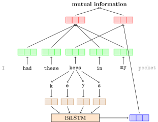
Figure 1: Architecture illustrated on the example text “had these keys in my” with target $Y=\mbox{``keys''}$.

5.4 Baselines

We focus on comparing with the following models which are some of the strongest baselines in the literature we are aware of. Berg-Kirkpatrick et al. (2010) extend a standard hidden Markov Model (HMM) to incorporate linguistic features. Stratos et al. (2016) develop a factorization-based algorithm for learning a constrained HMM. Ammar et al. (2014) propose a CRF autoencoder that reconstructs words from a structured label sequence. Lin et al. (2015) extend Ammar et al. (2014) by switching a categorical reconstruction distribution with a Gaussian distribution. In addition to these baselines, we also report results with Brown clustering (Brown et al., 1992), the Baum-Welch algorithm (Baum and Petrie, 1966), and $k$-means clustering of $300$-dimensional GloVe vectors Pennington et al. (2014).

5.5 Results

The 45-tag Penn WSJ dataset.

The 45-tag Penn WSJ dataset is a corpus of around one million words each tagged with one of $m=45$ tags. It is used to optimize hyperparameter values for all compared methods. Table 1 shows the average accuracy over $10$ random restarts with the best hyperparameter configurations; standard deviation is given in parentheses (except for deterministic methods Stratos et al. (2016) and Brown clustering).

Our model trained with the variational objective (7) outperforms all baselines. We also observe that our model trained with the generalized Brown objective (4) does not work. We have found that unless the minibatch size is as large as 10,000 the gradient steps do not effectively increase the true data-wide mutual information (4). This supports our bias analysis in Section 4. While it may be possible to develop techniques to resolve the difficulty, for instance keeping a moving average of estimates to stabilize estimation, we leave this as future work and focus on the variational objective in the remainder of the paper.

Method	Accuracy
Variational $\widehat{J}^{\mathrm{var}}$ (7)	$\boldsymbol{78.1}\;\mbox{(${\pm 0.8})$}$
Generalized Brown $\widehat{J}^{\mathrm{mi}}$ (4)	$48.8\;\;\mbox{(${\pm 0.9})$}$
Berg-Kirkpatrick et al. (2010)	$74.9\;\;\mbox{(${\pm 1.5})$}$
Stratos et al. (2016)	$67.7$
Brown et al. (1992)	$65.6$
Baum-Welch	$62.6\;\;\mbox{(${\pm 1.1})$}$
$k$-means	$32.6\;\;\mbox{(${\pm 0.7})$}$

Table 1: Many-to-one accuracy on the 45-tag Penn WSJ with the best hyperparameter configurations. The average accuracy over $10$ random restarts is reported and the standard deviation is given in parentheses (except for deterministic methods).

Table 2 shows ablation experiments on our best model (accuracy 80.1) to better understand the sources of its strong performance. Context size $H=2$ is a sizable improvement over $H=3$ or $H=1$. Random sampling is significantly more effective than sentence-level batching (i.e., each minibatch is the set of context-word pairs within a single sentence as done in McAllester (2018)). glove initialization of word embeddings $e_{w}$ is harmful. As expected for POS tagging, morphological modeling with LSTMs gives the largest improvement.

While it may be surprising that glove initialization is harmful, it is well known that pretrained word embeddings do not necessarily capture syntactic relationships (as evident in the poor performance of $k$-means clustering). Consider the top ten nearest neighbors of the word “made” under GloVe embeddings (840B.300d, within PTB vocab):

Cosine Similarity	Nearest Neighbor
0.7426	making
0.7113	make
0.6851	that
0.6613	they
0.6584	been
0.6574	would
0.6533	brought
0.6521	had
0.6514	came
0.6494	but
0.6486	even

The neighbors are clearly not in the same syntactic category. The embeddings can be made more syntactic by controlling the context window. But we found it much more effective (and much simpler) to start from randomly initialized embeddings and let the objective induce appropriate representations.

Configuration	Accuracy
Best	80.1
$H=3$	75.9
$H=1$	75.9
Sentence-level batching	72.4
glove initialization	67.6
No character encoding	65.6

Table 2: Ablation of the best model on Penn WSJ.

The 12-tag universal treebank.

The universal treebank v2.0 is a corpus in ten languages tagged with $m=12$ universal POS tags McDonald et al. (2013). We use this corpus to be compatible with existing results. Table 3 shows results on the dataset, using the same setting in the experiments on the Penn WSJ dataset. Our model significantly outperforms the previous state-of-the-art, achieving an absolute gain of 4.7 over Stratos et al. (2016) in average accuracy.

Method	de	en	es	fr	id	it	ja	ko	pt-br	sv	Mean
Variational $\widehat{J}^{\mathrm{var}}$ (7)	($\pm$1.5) 75.4	($\pm$1.7) 73.1	($\pm$1.0) 73.1	($\pm$2.9) 70.4	($\pm$1.5) 73.6	($\pm$3.3) 67.4	($\pm$0.4) 77.9	($\pm$1.2) 65.6	($\pm$2.3) 70.7	($\pm$1.5) 67.1	71.4
Stratos et al.	63.4	71.4	74.3	71.9	67.3	60.2	69.4	61.8	65.8	61.0	66.7
Berg-Kirkpatrick et al.	($\pm$1.8) 67.5	($\pm$3.5) 62.4	($\pm$3.1) 67.1	($\pm$4.5) 62.1	($\pm$3.9) 61.3	($\pm$2.9) 52.9	($\pm$2.9) 78.2	($\pm$3.6) 60.5	($\pm$2.2) 63.2	($\pm$2.5) 56.7	63.2
Brown et al.	60.0	62.9	67.4	66.4	59.3	66.1	60.3	47.5	67.4	61.9	61.9
Baum-Welch	($\pm$4.8) 45.5	($\pm$3.4) 59.8	($\pm$2.2) 60.6	($\pm$3.6) 60.1	($\pm$3.1) 49.6	($\pm$2.6) 51.5	($\pm$2.1) 59.5	($\pm$0.6) 51.7	($\pm$3.7) 59.5	($\pm$3.0) 42.4	54.0

Table 3: Many-to-one accuracy on the 12-tag universal treebank dataset. We use the same setting in Table 1. All models use a fixed hyperparameter configuration optimized on the 45-tag Penn WSJ.

Comparison with CRF autoencoders.

Table 4 shows a direct comparison with CRF autoencoders (Ammar et al., 2014; Lin et al., 2015) in many-to-one accuracy and the V-measure. We compare against their reported numbers by running our model once on the same datasets using the same setting in the experiments on the Penn WSJ dataset. The data consists of the training portion of CoNLL-X and CoNLL 2007 labeled with 12 universal tags. Our model is competitive with all baselines.

Metric	Method	Arabic	Basque	Danish	Greek	Hungarian	Italian	Turkish	Mean
M2O	Variational $\widehat{J}^{\mathrm{var}}$ (7)	74.3	70.4	71.7	66.1	61.2	67.4	64.2	67.9
	Ammar et al.	69.1	68.1	60.9	63.5	57.1	60.4	60.4	62.8
	Berg-Kirkpatrick et al.	66.8	66.2	60.0	60.2	56.8	64.1	62.0	62.3
	Baum-Welch	49.7	44.9	42.4	39.2	45.2	39.3	52.7	44.7
VM	Variational $\widehat{J}^{\mathrm{var}}$ (7)	56.9	43.6	56.0	56.3	47.9	53.3	38.5	50.4
	Lin et al.	50.5	51.7	51.3	50.0	55.9	46.3	43.1	49.8
	Ammar et al.	49.1	41.1	46.1	49.1	41.1	43.1	35.0	43.5
	Berg-Kirkpatrick et al.	33.8	33.4	41.1	40.9	39.0	46.6	31.6	38.8
	Baum-Welch	15.3	8.2	11.1	9.6	10.1	9.9	11.6	10.8

Table 4: Comparison with the reported results with CRF autoencoders in many-to-one accuracy (M2O) and the V-measure (VM).

6 Related Work

Information theory, in particular mutual information, has played a prominent role in NLP (Church and Hanks, 1990; Brown et al., 1992). It has intimate connections to the representation learning capabilities of neural networks (Tishby and Zaslavsky, 2015) and underlies many celebrated modern approaches to unsupervised learning such as generative adversarial networks (GANs) (Goodfellow et al., 2014).

There is a recent burst of effort in learning continuous representations by optimizing various lower bounds on mutual information (Belghazi et al., 2018; Oord et al., 2018; Hjelm et al., 2018). These representations are typically evaluated on extrinsic tasks as features. In contrast, we learn discrete representations by optimizing a novel generalization of the Brown clustering objective (Brown et al., 1992) and a variational lower bound on mutual information proposed by McAllester (2018). We focus on intrinsic evaluation of these representations on POS induction. Extrinsic evaluation of these representations in downstream tasks is an important future direction.

The issue of biased stochastic gradient estimators is a common challenge in unsupervised learning (e.g., see Wang et al., 2015). This arises mainly because the objective involves a nonlinear transformation of all samples in a training dataset, for instance the whitening constraints in deep canonical correlation analysis (CCA) (Andrew et al., 2013). In this work, the problem arises because of entropy. This issue is not considered in the original work of McAllester (2018) and the error analysis we present in Section 4 is novel. Our finding is that the feasibility of stochastic optimization greatly depends on the size of the bias in gradient estimates, as we are able to effectively optimize the variational objective while not the generalized Brown objective.

Our POS induction system has some practical advantages over previous approaches. Many rely on computationally expensive structured inference or pre-optimized features (or both). For instance, Tran et al. (2016) need to calculate forward/backward messages and is limited to truncated sequences by memory constraints. Berg-Kirkpatrick et al. (2010) rely on extensively hand-engineered linguistic features. Ammar et al. (2014), Lin et al. (2015), and He et al. (2018) rely on carefully pretrained lexical representations like Brown clusters and word embeddings. In contrast, the model presented in this work requires no expensive structured computation or feature engineering and uses word/character embeddings trained from scratch. It is easy to implement using a standard neural network library and outperforms these previous works in many cases.

Appendix A Proof of Theorem 4.1

We first analyze the variational loss

$$\widehat{H}(q,p)-\widehat{H}(Z)$$

Note that the cross entropy term decomposes over samples and causes no bias. Thus we focus on the negative entropy term

$$-\widehat{H}(Z)=\sum_{z}\hat{q}(z)\log\hat{q}(z)$$

whose gradient with respect to $q$ is

$$\sum_{z}\left(1+\log\hat{q}(z)\right)\nabla\hat{q}(z)$$

$$=\frac{1}{K}\sum_{k=1}^{K}\sum_{z}\left(1+\log\hat{q}(z)\right)\nabla\hat{q}_{k}(z)$$ (9)

where we expand $\nabla\hat{q}(z)$ by the identity

$$\nabla\hat{q}(z)=\frac{1}{N}\sum_{i=1}^{N}\nabla q(z|y_{i})=\frac{1}{K}\sum_{k=1}^{K}\nabla\hat{q}_{k}(z)$$ (10)

In contrast, the gradient of the negative entropy term averaged over minibatches is

$$\frac{1}{K}\sum_{k=1}^{K}\sum_{z}\left(1+\log\hat{q}_{k}(z)\right)\nabla\hat{q}_{k}(z)$$ (11)

Hence the difference between (9) and (11) is

$$\frac{1}{K}\sum_{k=1}^{K}\sum_{z}\log\frac{\hat{q}(z)}{\hat{q}_{k}(z)}\nabla\hat{q}_{k}(z)$$

This shows the first result. Now we analyze the generalized Brown loss

$$\frac{1}{N}\sum_{i=1}^{N}\sum_{z,z^{\prime}}p(z|x_{i})q(z^{\prime}|y_{i})\log\frac{\hat{p}(z)\hat{q}(z^{\prime})}{p(z|x_{i})q(z^{\prime}|y_{i})}$$

When we expand the log fraction, we see that the denominator decomposes over samples and causes no bias. Thus we focus on the numerator term

$$\frac{1}{N}\sum_{z,z^{\prime}}\log\left(\hat{p}(z)\hat{q}(z^{\prime})\right)\sum_{i=1}^{N}p(z|x_{i})q(z^{\prime}|y_{i})$$

By the product rule, its gradient with respect to $q$ is a sum of two terms. The first term is (using (10) again)

$$\frac{1}{N}\sum_{k=1}^{K}\sum_{z,z^{\prime}}\left(\frac{1}{K}\sum_{i=1}^{N}\frac{p(z|x_{i})q(z^{\prime}|y_{i})}{\hat{q}(z^{\prime})}\right)\nabla\hat{q}_{k}(z^{\prime})$$ (12)

The second term is (as a sum over batches)

$$\frac{1}{N}\sum_{k=1}^{K}\sum_{z,z^{\prime}}\log\left(\hat{p}(z)\hat{q}(z^{\prime})\right)\sum_{(x,y)\in B_{k}}p(z|x)\nabla q(z^{\prime}|y)$$ (13)

In contrast, the numerator term estimated as an average over minibatches is

$$\frac{1}{N}\sum_{k=1}^{K}\sum_{z,z^{\prime}}\log\left(\hat{p}_{k}(z)\hat{q}_{k}(z^{\prime})\right)\sum_{(x,y)\in B_{k}}p(z|x)q(z^{\prime}|y)$$

and the two terms of its gradient with respect to $q$ (corresponding to (12) and (13)) are

$$\frac{1}{N}\sum_{k=1}^{K}\sum_{z,z^{\prime}}\left(\sum_{(x,y)\in B_{k}}\frac{p(z|x)q(z^{\prime}|y)}{\hat{q}_{k}(z^{\prime})}\right)\nabla\hat{q}_{k}(z^{\prime})$$ (14)

$$\frac{1}{N}\sum_{k=1}^{K}\sum_{z,z^{\prime}}\log\left(\hat{p}_{k}(z)\hat{q}_{k}(z^{\prime})\right)\sum_{(x,y)\in B_{k}}p(z|x_{i})\nabla q(z^{\prime}|y)$$ (15)

Thus the difference between (12) and (14) is

$$\frac{1}{N}\sum_{k=1}^{K}\sum_{z,z^{\prime}}\epsilon_{k}(z,z^{\prime})\nabla\hat{q}_{k}(z^{\prime})$$

where

$$\epsilon_{k}(z,z^{\prime})= \frac{1}{K}\sum_{i=1}^{N}\frac{p(z|x_{i})q(z^{\prime}|y_{i})}{\hat{q}(z^{\prime})}$$

$$-\sum_{(x,y)\in B_{k}}\frac{p(z|x)q(z^{\prime}|y)}{\hat{q}_{k}(z^{\prime})}$$

The difference between (13) and (15) is

$$\frac{1}{N}\sum_{k=1}^{K}\sum_{z,z^{\prime}}\log\frac{\hat{p}(z)\hat{q}(z^{\prime})}{\hat{p}_{k}(z)\hat{q}_{k}(z^{\prime})}\sum_{(x,y)\in B_{k}}p(z|x)\nabla q(z^{\prime}|y)$$

Adding these differences gives the second result.

References

- Ammar et al. (2014) Waleed Ammar, Chris Dyer, and Noah A Smith. 2014. Conditional random field autoencoders for unsupervised structured prediction. In Advances in Neural Information Processing Systems, pages 3311–3319.
- Andrew et al. (2013) Galen Andrew, Raman Arora, Jeff Bilmes, and Karen Livescu. 2013. Deep canonical correlation analysis. In Proceedings of the 30th International Conference on Machine Learning, pages 1247–1255.
- Artstein (2017) Ron Artstein. 2017. Inter-annotator agreement. In Handbook of linguistic annotation, pages 297–313. Springer.
- Baum and Petrie (1966) Leonard E. Baum and Ted Petrie. 1966. Statistical inference for probabilistic functions of finite state Markov chains. The Annals of Mathematical Statistics, 37(6):1554–1563.
- Belghazi et al. (2018) Mohamed Ishmael Belghazi, Aristide Baratin, Sai Rajeshwar, Sherjil Ozair, Yoshua Bengio, Aaron Courville, and Devon Hjelm. 2018. Mutual information neural estimation. In Proceedings of the 35th International Conference on Machine Learning, pages 531–540.