A New Formulation of The Shortest Path Problem with On-Time Arrival Reliability

Abstract

We study stochastic routing in the PAth-CEntric (PACE) uncertain road network model. In the PACE model, uncertain travel times are associated with not only edges but also some paths. The uncertain travel times associated with paths are able to well capture the travel time dependency among different edges. This significantly improves the accuracy of travel time distribution estimations for arbitrary paths, which is a fundamental functionality in stochastic routing, compared to classic uncertain road network models where uncertain travel times are associated with only edges.

We investigate a new formulation of the shortest path with on-time arrival reliability (SPOTAR) problem under the PACE model. Given a source, a destination, and a travel time budget, the SPOTAR problem aims at finding a path that maximizes the on-time arrival probability. We develop a generic algorithm with different speed-up strategies to solve the SPOTAR problem under the PACE model. Empirical studies with substantial GPS trajectory data offer insight into the design properties of the proposed algorithm and confirm that the algorithm is effective.

This report extends the paper “Stochastic Shortest Path Finding in Path-Centric Uncertain Road Networks”, to appear in IEEE MDM 2018, by providing a concrete running example of the studied SPOTAR problem in the PACE model and additional statistics of the used GPS trajectories in the experiments.

I Introduction

Emerging transportation innovations, such as mobility-on-demand services and autonomous driving, call for stochastic routing where travel time distributions, but not just average travel times, are utilized [1, 2]. For example, consider two paths $P_{1}$ and $P_{2}$ where both paths connect the same source and destination. The travel time distribution of the two paths are shown in Table I.

Travel time (mins)	40	50	60	70
$P_{1}$	0.5	0.2	0.2	0.1
$P_{2}$	0	0.8	0.2	0

TABLE I: Travel Time Distributions for $P_{1}$ and $P_{2}$

If only considering average travel times, $P_{1}$ is always the best choice, because $P_{1}$ has average travel time 49 whereas $P_{2}$’s average travel time is 52. However, if a person needs to go to the destination within 60 minutes, e.g., to catch a flight, then $P_{2}$ is the best choice as it guarantees that the person will arrive the destination within 60 minutes. In contrast, taking $P_{1}$ may run into a risk that the person will miss the flight when the path takes 70 minutes.

In this paper, we consider stochastic routing that takes into account travel time distributions. In particular, we investigate the shortest path with on-time arrival reliability (SPOTAR) problem. Given a source, a destination, and a travel time budget, e.g., 60 minutes, the SPOTAR problem aims at finding a path that maximizes the on-time arrival probability, i.e., the probability of arriving the destination within the time budget.

Although the SPOTAR problem has been studied in the literature [4, 5], they all consider a classical uncertain road network modeling, where uncertain travel times are assigned to only edges, and the uncertain travel times on different edges are independent. We call the classical model the edge-centric model. However, recent studies suggest that the travel times on different edges are often highly dependent [2, 3]. The edge-centric model ignores the dependency and thus results in inaccurate travel time distribution computation for paths, especially for long paths. To contend with this, a PAth-CEntric model (PACE) has been proposed [2, 3]. In the PACE model, not only edges, but some paths are also associated with uncertain travel times and the uncertain travel times that are associated with paths well capture the dependency of the travel times among different edges in the path. Thus, the PACE model is able to provide much more accurate travel time distributions [2, 3]. However, existing algorithms that work for the edge-centric model cannot be applied directly in the new PACE model. In this paper, we investigate how to solve the SPOTAR problem under the PACE model.

Contributions: To the best of our knowledge, this is the first paper to study the SPOTAR problem in the PACE model that exploits travel time dependencies among edges. First, we define the SPOTAR problem in the PACE model. Second, we propose a generic algorithm with different speed-up heuristics to solve the problem. Third, we report on comprehensive experiments based on real world trajectory data.

II Related work

We first review two uncertain road network models and then discuss existing studies on stochastic shortest path finding.

Uncertain Road Network Modeling: The edge-centric uncertain road network model has been applied extensively in stochastic routing [4, 5, 7, 8, 9, 10, 11, 12, 13, 14, 15, 16]. In the edge-centric model, each edge is associated with an uncertain travel time and different edges’ uncertain travel times are independent. Given a path, the uncertain time of the path is derived by convoluting the uncertain times of the edges in the path. However, uncertain travel times among different edges in a path are often dependent but not independent. The edge-centric model is unable to capture the dependency and thus results in inaccurate uncertain travel times for paths. To contend with this, the PAth-CEntric (PACE) model is proposed recently [2, 3]. PACE also associates some paths with joint travel time distributions that well capture the dependency of the uncertain travel times of the edges in the paths.

Stochastic shortest path finding: There exist two categories of stochastic shortest path finding—the Shortest path with on-time arrival reliability problem (SPOTAR) and the Stochastic on time arrival problem (SOTA) [4, 5]. SPOTAR identifies an a-priori path that maximizes the on time arrival reliability of reaching a destination within a pre-defined time budget. SOTA considers a scenario where a vehicle keeps moving and needs to choose which edge to follow at each intersection, based on the travel time has been already spent. SOTA tries to find an optimal policy that guides a vehicle to choose the next optimal edge at each intersection. We study the SPOTAR problem in the PACE model, while exsiting studies on SPOTAR all consider the edge-centric model.

III Preliminaries

We use a graph to model a road network. In particular, a road network is modeled as a directed graph $G=(V,E)$. $V$ is a set of nodes that represent intersections and $E\subseteq V\times V$ is a set of edges that represent road segments. For example, Figure 1 shows a graph that models a road network with 6 intersections (i.e., nodes) and 9 road segments (i.e., edges).

A path is a sequence of adjacent edges $P=\langle e_{1},e_{2}$, $\ldots$, $e_{n}\rangle$, where $n\geq 1$. In addition, we require that the edges in path $P$ are unique, meaning that $e_{i}\neq e_{j}$, if $1\leq i,j\leq n$ and $i\neq j$. Next, we define a subsequence of edges in path $P$ as its sub-path $P^{\prime}$. Formally, $P^{\prime}=\langle e_{i},e_{i+1}$, $\ldots$, $e_{j-1}$, $e_{j}\rangle$, where $1\leq i<j\leq n$. For example, in Figure 1, path $P_{1}=\langle e_{1},e_{4}\rangle$ is a sub-path of path $P_{2}=\langle e_{1},e_{4},e_{9}\rangle$.

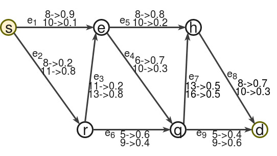
Figure 1: Road Network and Uncertain Edge Weights

Based on the above definitions, we proceed to introduce the classic edge-centric uncertain road network model and the path-centric uncertain road network model (i.e., PACE), respectively.

Edge-centric uncertain road network model: We maintain a weight function $W$ that takes as input an edge and returns an uncertain travel time for the edge. We maintain an uncertain travel time for each edge. The edge-centric model is considered as the de-facto model in stochastic routing [4, 5, 6, 7, 8, 9, 16].

The uncertain edge weights are often instantiated using trajectories that occurred on the road network. Given a set of trajectories, we first break the trajectories to small pieces that fit the underlying edges and then use the small pieces to instantiate edge weights.

Assume that there we have 100 trajectories as shown in Table II. The first row of Table II means that 80 trajectories traversed path $\langle e_{1},e_{4}\rangle$, which spent 8 mins on $e_{1}$ and 6 mins on $e_{4}$.

Traversed Path	Costs on edges	# of trajectories
$\langle e_{1},e_{4}\rangle$	8, 6	80
$\langle e_{1},e_{4}\rangle$	10, 10	20
$\langle e_{1}\rangle$	8	100

TABLE II: Trajectory Examples

Now, we are able to instantiate $W(e_{1})=\{(8,0.9)$, $(10,0.1)\}$, meaning that $e_{1}$ may take 8 mins with probability 0.9, and 10 mins with probability 0.1, as shown in Fig. 1. This is because out of 200 trajectories that traversed $e_{1}$, 180 trajectories took 8 mins and 20 trajectories took 10 mins. Similarly, we have $W(e_{4})=\{(6,0.8),(10,0.2)\}$.

In this edge-centric model, the uncertain travel times of edges are independent. Thus, the uncertain travel time of a path is computed as the convolution of the uncertain travel times of the edges in the path [4, 5, 6, 7, 8, 9, 16]. For example, assuming that we have instantiated the edge weights as shown in Figure 1. Consider path $P_{1}=\langle e_{1},e_{4}\rangle$. Since we assume that the travel times of $e_{1}$ and $e_{4}$ are independent, we compute the joint travel time distribution first. Then, based on the joint distribution, we are able to compute the total travel time distribution, which is shown in Table III.

$e_{1}$	$e_{4}$	Probability
8	6	0.63
8	10	0.27
10	6	0.07
10	10	0.03

(a) Joint Travel Time Distribution

$P_{1}$	Probability
14	0.63
18	0.27
16	0.07
20	0.03

(b) Total Travel Time Distribution

TABLE III: Joint vs. Total Travel Time Distribution

Note that the computed total travel time distribution of path $P_{1}$ is inconsistent with the “ground truth” distribution that is reflected in the trajectories in Table II. The ground truth distribution suggests $P_{1}$ took 14 mins with probability 0.8 (because out of 100 trajectories, 80 trajectories took 14 mins to traverse $P_{1}$) and 20 mins with probability 0.2 (because out of 100 trajectories, 20 trajectories took 20 mins to traverse $P_{1}$). This example shows that the travel time dependency, i.e., traveling fast/slow on $e_{1}$ and also traveling fast/slow on $e_{2}$, is broken when using the edge-centric model, which results in inaccurate uncertain travel time for paths. It also shows that it is very important to use trajectories that are traversing the whole path, but not only intendant edges when calculating the travel cost distribution of a path.

PAth-CEntric (PACE) uncertain road network model: In the PACE model [2, 3], not only edges are associated with uncertain travel times, some paths are also associated with uncertain travel times. The uncertain travel times that are associated with paths model the joint travel time distributions of the edges in the paths.

Following the running example, PACE maintains not only uncertain travel times for edges, i.e., $W(e_{1})$ and $W(e_{4})$, but also the joint travel time distribution for path $P_{1}$, i.e., $W(P_{1})$, as shown Table IV(a). The joint travel time distributions maintained in PACE are directly derived from trajectories. Based on $W(P_{1})$, we are able to derive total travel time distribution of $P_{1}$, which well aligns with the ground truth distribution.

$e_{1}$	$e_{4}$	Probability
8	6	0.8
10	10	0.2

(a) $W(P_{1})$

$P_{1}$	Probability
14	0.8
20	0.2

(b) Total Travel Time Distribution

TABLE IV: Joint Distributions in PACE

Note that, in PACE, only some paths are associated with uncertain travel times, but not all paths. A road network may have a huge number of meaningful paths and thus we cannot afford maintain uncertain travel times for all paths in PACE. In addition, we often lack sufficient trajectories to cover all paths. In practice, we maintain joint distributions for those paths which have been traversed by sufficient amount of trajectories, e.g., popular paths.

Next, we present how to compute the travel time distribution of a path in PACE by using a concrete example. Assuming that, in addition to path travel time distribution $W(P_{1})$, PACE also maintains path travel time distribution $W(P_{2})$ for path $P_{2}=\langle e_{4},e_{9}\rangle$. Then, given a path $P=\langle e_{1},e_{4},e_{9}\rangle$, there exist more than one combination of weights such that each combination covers $P$. For example, we may use $\{W(e_{1})$, $W(e_{4})$, $W(e_{9})\}$, $\{W(e_{1})$, $W(P_{2})\}$, $\{W(P_{1})$, $W(e_{9})\}$, and $\{W(P_{1})$, $W(P_{2})\}$ to compute $P$’s uncertain travel time, respectively. It has been shown that the coarsest combination, i.e., the combination with the longest sub-paths, gives the most accurate uncertain travel time [2, 3]. In our example, it is $\{W(P_{1})$, $W(P_{2})\}$.

After identifying the coarsest combination for a query path $P$, say $\{P_{1},P_{2},\ldots,P_{n}\}$, we use Equation 1 to compute the joint distribution of $P$ [2, 3].

$$prob(P)=\frac{\Pi_{i=1}^{n}W(P_{i})}{\Pi_{i=1}^{n-1}W(P_{i}\cap P_{i+1})}$$ (1)

where $P_{i}\cap P_{i+1}$ denotes the overlapped path of paths $P_{i}$ and $P_{i+1}$. Consider the running example where $P=\langle e_{1},e_{4},e_{9}\rangle$. We have $prob(P)=\frac{W(P_{1})\cdot W(P_{2})}{W(\langle e_{4}\rangle)}$ since $P_{1}\cap P_{2}=\langle e_{4}\rangle$.

Problem Definition: Given a source vertex $v_{s}$, a destination vertex $v_{d}$, and a travel time budget $T$, we aim at identifying path $P^{*}$ which goes from $v_{s}$ to $v_{d}$ and has the largest probability of arriving the destination $v_{d}$ within the time budget $T$. This means that $P^{*}=\arg\max_{P\in\mathit{Path}}\mathit{Prob}(P.\mathit{TravelTime}\leq T)$, where set $\mathit{Path}$ contains all paths from $v_{s}$ to $v_{d}$ and the travel time distribution of path $P$ is computed using the PACE model.

IV Proposed Solution

We propose an algorithm for solving the SPOTAR problem based on the PACE model. The algorithm is based on a heuristic function that estimates the least possible travel time from a vertex to the destination vertex. We first introduce the heuristic function and then introduce the algorithm using the heuristic function.

IV-A Heuristic Function

Motivated by $A^{*}$ algorithm, to decide which edge we need to explore next to find the SPOTAR path, we maintain a heuristic function that takes as input a vertex and returns the least possible travel time from the vertex to the destination vertex $v_{d}$.

A baseline heuristic function can simply return a travel time that equals to the Euclidean distance between the argument vertex and $v_{d}$ divided by the maximum speed limit in the road network. However, this heuristic is too optimistic and thus loose. We aim at introducing a tighter heuristic.

To this end, we first introduce a reversed graph $G_{rev}=(V,E^{\prime})$ based on the original graph $G=(V,E)$ and then compute a shortest path tree that is rooted at $v_{d}$ in $G_{rev}$. In particular, $G_{rev}$ contains the same vertices with $G$ and the edges in $G_{rev}.E^{\prime}$ have reversed directions of the edges in $G.E$. Fig. 2 shows the reversed graph of the graph shown in Fig. 1. In the reversed graph, the edge weights are deterministic. In particular, for an edge $e^{\prime}=(v_{i},v_{j})\in E^{\prime}$, its weight equals to the least travel time of the uncertain travel time on edge $e=(v_{j},v_{i})\in E$ in the original graph. For example, edge $e_{1}^{\prime}$ in $G_{rev}$ has weight 8 since the least travel time of edge $e_{1}$ in $G$ is 8.

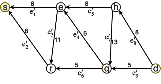
Figure 2: Reversed Graph $G_{rev}$ of $G$

Next, we compute a shortest path tree that is rooted as the destination vertex $v_{d}$ in the reversed graph $G_{rev}$ using Dijkstra’s algorithm. Note that Dijkstra’s algorithm finishes when the distance from the destination vertex to a vertex becomes higher than the time budget $T$. In other words, we do not need to compute a full shortest path tree but only part of the shortest path tree that contains the vertices whose distances to $v_{d}$ are not larger than $T$. We use function $v_{i}.getMin()$ to return the minimum travel time which is needed to travel from $v_{i}$ to destination $v_{d}$.

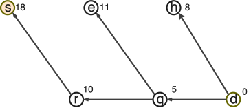
Figure 3: The Reversed Shortest Path Tree With Root $d$

Figure 3 shows the reversed shortest path tree rooted at vertex $v_{d}$ with budget $T=20$. If budget is 15, the shortest path tree excludes edge $\langle r,s\rangle$. And we have $v_{e}.getMin()=11$ meaning that it took at least 11 mins to travel from $v_{e}$ to destination $v_{d}$.

Based on the reversed shortest path tree, we derive the “best” travel time distribution of reaching destination vertex $v_{d}$ from any vertex $v_{i}$ within $t$ time units as $u_{i}(t)$, which is shown in Equation 4.

$$u_{i}(t)=\begin{cases}1&\text{if $t\geq v_{i}.getMin()$}\\ 0&\text{if $t<v_{i}.getMin()$}\end{cases}$$ (2)

Given a path $P$ from source vertex $v_{s}$ to vertex $v_{i}$, we are able to compute the cost distribution of path $P$ using the PACE model. Now, based on best travel time distribution $u_{i}(t)$, we are able to estimate the best travel time distribution if we follow $P$ and continue to reach the destination $v_{d}$. In particular, we use $r_{i}^{P}(x)$ to denote the largest probability of arriving the destination $v_{d}$ within $x$ mins if we follow path $P$ to go from $v_{s}$ to $v_{i}$ and then reach the destination $v_{d}$.

$$r_{i}^{P}(x)=\sum\limits_{k=1}^{x}prob_{P}(k).u_{i}(x-k)$$ (3)

where $prob_{P}(k)$ indicates the probability that $P$ takes $k$ mins and $u_{i}(x-k)$ indicates the probability that it takes less than $x-k$ mins to go from $v_{i}$ to $v_{d}$.

IV-B Proposed Algorithm

The algorithm for computing the SPOTAR problem is shown in Algorithm 1.

Algorithm 1 SolveSPOTAR(Vertex $v_{s}$, Vertex $v_{d}$, TimeBudget $T$)

1:  Initialize a priority queue $Q$;

2:  Path $P^{*}\leftarrow null$; double $maxProb\leftarrow 0$;

3:  for $v_{i}\in$ all vertices that can be reached from $v_{s}$ do

4:     $siJoint\leftarrow W(v_{s},v_{i})$, $siCost\leftarrow W(v_{s},v_{i})$;

5:     if $MinCost(siCost)+v_{i}.getMin()\leq T$ then

6:        $r\leftarrow r_{i}^{\langle(v_{s},v_{i})\rangle}(T)$ based on Eq. 3;

7:        $Q.Push(r,(\langle(v_{s},v_{i})\rangle,siJoint,siCost))$;

8:     end if

9:  end for

10:  while $Q$ is not empty do

11:     $(r,(P,pathJoint,pathCost))\leftarrow Q.ExtracMax()$;

12:     $v_{i}\leftarrow$ last vertex in path $P$;

13:     if $v_{i}==v_{d}$ then

14:        if $r>maxProb$ then

15:           $P^{*}\leftarrow P$; $maxProb\leftarrow r$;

16:           Delete all elements whose $r$ values are smaller than the current $r$ from $Q$;

17:           Continue;

18:        else

19:           Break;

20:        end if

21:     end if

22:     for $v_{k}\in$ all vertices that can be reached from $v_{i}$ do

23:        if Path $P$ has not traversed $v_{k}$ yet then

24:           $extP\leftarrow P\oplus(v_{i},v_{k})$;

25:           $ikMin\leftarrow MinCost(v_{i},v_{k})$ ;

26:           $pathMin\leftarrow MinCost(pathCost)$;

27:           if $ikMin+pathMin+j.getMin()\leq T$ then

28:              $extPJoint\leftarrow PACE(extP)$;

29:              $extPCost\leftarrow JointToCost(extPJoint)$;

30:              $r\leftarrow r_{k}^{extP}(T)$ based on Eq. 3;

31:              if $CheckStochasticDominance()$ then

32:                 $Q.Push(r,(extP,extPJoint,extPCost))$

33:              end if

34:           end if

35:        end if

36:     end for

37:  end while

38:  return path $P^{*}$;

We start initializing a priority queue $Q$ that holds elements in the form of $(r,(P,pathJoint,pathCost))$, where $P$ is a path from source $v_{s}$ to some vertex $v_{i}$, $r=r_{i}^{P}(T)$ is the largest probability of arriving $v_{d}$ within time budget $T$ using path $P$, $pathJoint$ is the joint distribution of $P$, and $pathCost$ is the total travel time distribution of $P$. We also initialize path $P^{*}$, which intends to maintain a candidate SPOTAR path and its probability $maxProb$ of arriving destination $v_{d}$.

We first check all vertices that are from vertex $v_{s}$ (line 3 to line 7). Since now the candidate path $\langle(v_{s},v_{i})\rangle$ only has one edge, the joint distribution and cost distribution are the same (line 4). Next, if the minimum travel time from the candidate path to $v_{d}$ is already larger than the time budget $T$, we do not insert it into the priority queue. Otherwise, we insert it.

We proceed to the main while loop at line 10: in each iteration, we extract the element with the largest $r$ value until the priority queue $Q$ is empty.

Assume that the element with the largest $r$-value represents path $P$. We check if $P$ has already arrived destination $v_{d}$. If yes, we check if $P$’s $r$-value is larger than the current maximum probability $maxProb$. If yes, we update the candidate SPOTAR path $P^{*}$ and remove all the elements from $Q$ if their $r$-values are smaller than the current $r$. If not, we can stop the algorithm since all the remaining paths in the priority queue have $r$-values less than the current maximum probability $maxProb$. This means it makes no sense to keep exploring the remaining paths, since their probabilities of arriving $v_{d}$ within time budget $T$ cannot be greater than $maxProb$.

On the other hand, if $P$ has not arrived at $v_{d}$ yet, i.e., $v_{i}\neq v_{d}$, we need to extend $P$ by one more edge $(v_{i},v_{k})$ to get an extended path $extP$, which arrives vertex $v_{k}$. Here, we only consider simple path without cycles as it has been shown that a path with cycles cannot be a SPOTAR path [6].

If it is possible to follow $extP$ to arrive $v_{d}$ within the time budge $T$, we compute its joint distribution $extPJoint$ using the PACE model and its total cost distribution $extPCost$. We next apply Equation 3 to compute the $r$- value of the extend path $extP$.

Before inserting the extended path $extP$ into the priority queue $Q$, we need to conduct the following stochastic dominance check. If there already exists a path $P_{k}$ in $Q$ which also arrives $v_{k}$. We check if $extP$’s cost distribution stochastic dominanates [8] $P_{k}$’s cost distribution. If yes, we remove $P_{k}$’s element from $Q$ and insert $(r$, $(extP$, $extPJoint$, $extPCost))$ into $Q$. Similarly, if $P_{k}$ stochastic dominates $extP$, we do not need to insert $extP$ into $Q$. Note that only considering if $extP$’s $r$-value is larger than $P_{k}$’s $r$-value is insufficient [4, 8].

Finally, we return the SPOTAR path $P^{*}$ along with the maximum probability of arriving $v_{d}$ within time budget $T$.

V Running example

This section presents a concrete example of the SPOTAR problem which is solved by the proposed algorithm. The graph from Figure 1 is used to show a running example of the Algorithm for computing SPOTAR under the PACE model [1]. The joint distribution and the derived cost distribution for paths $<e_{1},e_{4}>$ and $<e_{2},e_{6}>$ for the graph in Fig. 1 are shown in TablesV and VI, respectively. For example, the joint distribution for path $<e_{1},e_{4}>$ has been derived from the trajectories shown in Table II.

$e_{1}$	$e_{4}$	Probability
8	6	0.8
10	10	0.2

(a) $W(P_{<e_{1},e_{4}>})$

$P_{e_{1},e_{4}}$	Probability
14	0.8
20	0.2

(b) Total Cost Distribution

TABLE V: Joint vs. total cost distributions for path $<e_{1},e_{4}>$

$e_{2}$	$e_{6}$	Probability
8	5	0.7
11	9	0.3

(a) $W(P_{<e_{2},e_{6}>})$

$P_{e_{2},e_{6}}$	Probability
13	0.7
20	0.3

(b) Total Cost Distribution

TABLE VI: Joint vs. total cost distributions for path $<e_{2},e_{6}>$

Problem: Consider a problem that aims at finding the path with the highest probability of reaching destination $d$ from source $s$ in a graph $G$ within a time budget $T=22$. In addition, we have $\delta=1$; and the following paths’ joint distributions are known a priori and is maintained in the path weight function $W$: $<e_{1},e_{4}>$ in Table V, $<e_{2},e_{6}>$ in Table VI

Solution: The reversed graph with minimum travel times for all edges is shown in Figure 2. Next, the algorithm computes the shortest path tree based on the graph, and labels each node with the distance to destination node $d$ as shown in Figure 3.

For each node $i$, we define $u_{i}(t)$ as the highest probability of reaching the destination node $d$ from node $i$, i.e., Equation 4 as stated in [1], where $i.GetMinVal()$ denotes the minimum travel time from node $i$ to destination node $d$ and $t$ is a given time budget.

$$u_{i}(t)=\begin{cases}1&\text{if $t\geq v_{i}.getMin()$}\\ 0&\text{if $t<v_{i}.getMin()$}\end{cases}$$ (4)

The algorithm begins with initialization of the priority queue $Q$. Next, it iterates over all adjacent arcs of $s$, i.e. $e_{1}$ and $e_{2}$. For arc $e_{1}$ the algorithm computes $prob_{e_{1}}$ which is given as follows:

$prob_{e_{1}}=${$(8,0.9),(10,0.1)$}

Next, the value of $r$ is computed using $u_{e}$ as follows:

$r=\sum\limits_{k=1}^{T}prob_{ei}(k).u_{e}(T-k)=\sum\limits_{k=1}^{T=22}prob_{e_{1}}(k).u_{e}(22-k)=prob_{e_{1}}(8).u_{e}(22-8)+prob_{e1}(10).u_{e}(22-10)=0.9*1+0.1*1=1$

After the value of $r$ has been computed, edge $e_{1}$ has been added to the path created until now, i.e., $<e_{1}>$. The path along with its $r$ value are pushed to the priority queue $Q$.

$Q.push(1.0,(<e_{1}>,prob_{e_{1}},cost_{e_{1}}))$

The second adjacent arc of node $s$ that has been considered by the algorithm is arc $e_{2}$. The algorithm again starts by computing the joint probability for the path discovered until now (i.e. $e_{2}$), which is shown as follows.

$prob_{e_{2}}=${$(8,0.2),(11,0.8)$}

Next, the algorithm computes $r$ values for node $r$ using $u_{r}=10$.

$r=\sum\limits_{k=1}^{T}prob_{e_{2}}(k).u_{r}(T-k)=\sum\limits_{k=1}^{T=22}prob_{e_{2}}(k).u_{e}(22-k)=prob_{e_{2}}(8).u_{r}(22-8)+prob_{e_{2}}(11).u_{r}(22-11)=0.2*1+0.8*1=1$

Once the r-value of $r$ has been computed, edge $e_{2}$ has been added to the path created until now and its value has been pushed to the priority queue $Q$ $Q.push(1.0,(<e_{2}>,prob_{e_{2}},cost_{e_{2}}))$

Next, the algorithm has to pop the value with the maximum key from the priority queue $Q$. Until now there are two elements in $Q$ i.e. edge $e_{1}$ and edge $e_{2}$ both with key value equal to 1. The algorithm decides to pop the element which is associated with the path $e_{1}$ based on the key $(1.0)$.

After that, the algorithm iterates over all adjacent arcs of node $e$ i.e. arcs $e_{5}$ and $e_{4}$.

For arc $e_{5}$ conditional independence holds because there are no overlapping sub-paths that contains $e_{5}$ and the path constructed so far by the algorithm. Therefore, the algorithm computes the joint distribution and then derive the associated cost distribution as shown in Table VII.

$prob_{e_{1},e_{5}}=prob_{e_{1}}\cdot prob_{e_{5}}$

$e_{1}$	$e_{5}$	Probability
8	8	0.72
8	10	0.18
10	8	0.08
10	10	0.02

(a) $W(P_{e_{1},e_{5}})$

$P_{e_{1},e_{5}}$	Probability
16	0.72
18	0.26
20	0.02

(b) Total Cost Distribution

TABLE VII: Joint and the derived cost distributions for path $<e_{1},e_{5}>$

Next, the algorithm prunes path $<e_{1},e_{5}>$ based on minimum travel time to destination $d$ i.e. $(16+8)>T=22$, therefore nothing has been added to priority queue.

The next adjacent arc of the path $<e_{1}>$ that ends in node $e$ is $e_{4}$. It passes through path $<e_{1},e_{4}>$, therefore the algorithm uses the given joint and cost distributions from Table V and then $r$ has been computed, where $u_{q}=5$.

$r=\sum\limits_{k=1}^{T}prob_{e_{1},e_{4}}(k).u_{q}(T-k)=\sum\limits_{k=1}^{22}prob_{e_{1},e_{4}}(k).u_{q}(22-k)=prob_{e_{1},e_{4}}(14).u_{q}(22-14)+prob_{e_{1},e_{4}}(20).u_{q}(22-20)=0.8*1+0.2*0=0.80$

The path $<e_{1},e_{4}>$ has been added to the priority queue $Q$.

$Q.push(0.8,(<e_{1},e_{4}>,prob_{e1,e4},cost_{e1,e4}))$

Until now, there are two paths in the priority queue i.e. path $<e_{2}>$ and path $<e_{1},e_{4}>$ with keys 1.0 and 0.8, respectively.

The algorithm pops the element associated with path $<e_{2}>$ from the priority queue based on the element keys since $1.0>0.8$.

Then the algorithm iterates over all adjacent arcs of $r$ i.e. $e_{3}$ and $e_{6}$. Arc $e_{3}$ can be pruned based on minimum travel time calculated as follows $(8+11)+11>T=22$. Since arc $e_{6}$ passes through path $<e_{2},e_{6}>$, the algorithm uses the given probability in Table VI in order to compute a value of $r$, where $u_{q}=5$ as follows:

$r=\sum\limits_{k=1}^{T}q_{e_{2},e_{6}}(k).u_{q}(T-k)=\sum\limits_{k=1}^{22}prob_{e_{2},e_{6}}(k).u_{q}(22-k)=prob_{e_{2},e_{6}}(13).u_{q}(22-13)+prob_{e_{2},e_{6}}(20).u_{q}(22-20)=0.7*1+0.3*0=0.70$

Since path $<e_{2},e_{6}>$ ends in node $q$ and path $<e_{1},e_{4}>$ also ends in node q and it is already added to the priority queue, we try to prune one of the paths based on Stochastic dominance as explained in [1].

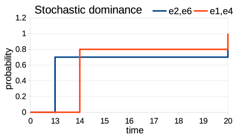
Figure 4: Stochastic dominance between paths $<e_{1},e_{2}>$ and $<e_{2},e_{6}>$. None of the paths stochastically dominates the other one.

As it can be seen from Figure 4, none of the path stochastically dominates the other, therefore we cannot prune either of them, hence the algorithm adds path $<e_{2},e_{6}>$ to the priority queue $Q$

$Q.push(0.70,(<e_{2},e_{6}>,prob_{e_{2},e_{6}},cost_{e_{2},e_{6}}))$

At this point the priority queue $Q$ contains two paths: $<e_{1},e_{4}>$ and $<e_{2},e_{6}>$ with the following objects associated as follows:

$(0.80,(<e_{1},e_{4}>,prob_{e_{1},e_{4}},cost_{e_{1},e_{4}})$

$(0.70,(<e_{2},e_{6}>,prob_{e_{2},e_{6}},cost_{e_{2},e_{6}})$

Path $<e_{1},e_{4}>$ has been popped up from the priority queue $Q$ based on its key 0.8 and for all adjacent edges of node $q$ i.e. arcs $e_{7}$ and $e_{9}$.

Arc $e_{7}$ is pruned by the algorithm bases on its minimum travel time to destination calculated as follows: $(14+13)+8>T=22$

Arc $e_{9}$ is explored by the algorithm, it computes the travel cost distribution for path $<e_{1},e_{4},e_{9}>$ where independence between $<e_{1},e_{4}>$ and $<e_{9}>$ does hold, the result can be seen in Table VIII

$e_{1}$	$e_{4}$	$e_{9}$	Probability
8	6	5	0.32
8	6	9	0.48
10	10	5	0.08
10	10	9	0.12

(a) $W(P_{e_{1},e_{4},e_{9}})$

$P_{e_{1},e_{4},e_{9}}$	Probability
19	0.32
23	0.48
25	0.08
29	0.12

(b) Total Cost Distribution

TABLE VIII: Joint vs. total cost distributions for path $<e_{1},e_{4},e_{9}>$

The search reaches a destination node $d$. Solution 1 for path $<e_{1},e_{4},e_{9}>$ with probability 0.32 of reaching the destination $d$ within a time budget of 22 units. After obtaining a solution. The algorithm checks the keys (i.e., the r-values) of all elements in priority queue. If the key is less then the probability of the solution $(0.32)$, we prune the corresponding entry from the priority queue. Since $0.70>0.32$, we therefore cannot prune path $<e_{2},e_{6}>$ which is in the priority queue.

Pop $<e_{2},e_{6}>$ based on key $0.70$. For all adjacent arcs of node $q$ First $e_{7}$ can be pruned based on minimum travel time $(13+13)+8>T=22$ Second, arc $e_{9}$. The algorithm computes the travel cost for the path $<e_{2},e_{6},e_{9}>$. Independence does hold, therefore therefore we have that $prob_{e_{2},e_{6},e_{9}}=prob_{e_{2},e_{6}}\cdot prob_{e_{9}}$ the result is shown in Table IX

$e_{2}$	$e_{6}$	$e_{9}$	Probability
8	5	5	0.28
8	5	9	0.42
11	9	5	0.12
11	9	9	0.18

(a) $W(P_{e_{2},e_{6},e_{9}})$

$P_{e_{2},e_{6},e_{9}}$	Probability
18	0.28
22	0.42
25	0.12
29	0.18

(b) Total Cost Distribution

TABLE IX: Joint vs. total cost distributions for path $<e_{2},e_{6},e_{9}>$

The search reaches destination node d. Solution $2$ for path $<e_{2},e_{6},e_{9}>$ with probability $0.70$ of reaching the destination node $d$ within a time budget $22$ units. We check the keys of all elements in priority queue. If the key is less then $0.70$, we eliminate the corresponding entry from the priority queue. Priority queue is empty, so we can not prune. Since solution 2 with path $<e_{2},e_{6},e_{9}>$ has higher probability of reaching the destination node $d$ within a time budget of $22$ units. It is the final solution.

VI Experimental results

We report on experimental results using real world GPS trajectories.

VI-A Experimental Setup

We use the road network of Aalborg, Denmark, which contains 6,253 nodes and 10,716 edges. We use 37 million GPS records that occurred in Aalborg from Jan 2007 to Dec 2008 to instantiate the PACE model. The sampling rate of GPS records is 1 Hz (i.e., one GPS record per second). If an edge is not covered by GPS data, we use the length of the edge and the speed limit on the edge to derive a travel time. If a path has been traversed by 10 trajectories, we maintain a joint distribution for the path. A visual representation of the edges that are covered and not covered by the GPS trajectories can be found in Figure 5.

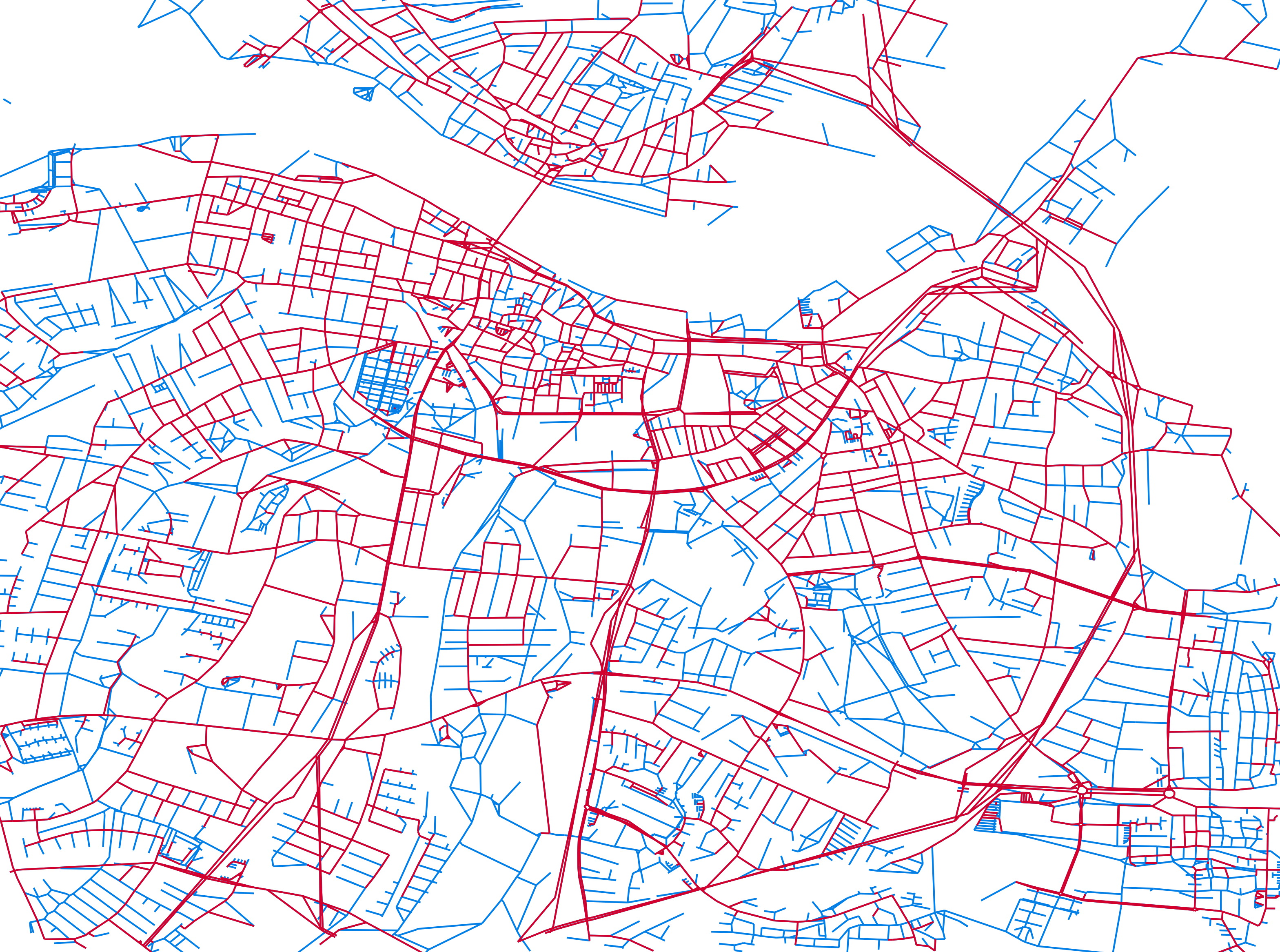
Figure 5: Aalborg network. The red segments are covered by the GPS trajectories and thus their travel cost distributions are derived from the GPS trajectories. The blue segments are not covered by the GPS trajectories and thus speed limits are used to derive travel costs.

Queries: We consider different settings to generate SPOTAR queries. We vary time budget (seconds) from 300, 500, 700, to 1,000. We also vary the Euclidean distance (km) between source-destination pairs: $[0,1)$, $[1,2)$, $[2,3)$, and $[3,4)$. For each setting, we randomly generate 20 source-destination pairs.

Methods: We consider different heuristic functions: (1) the proposed solution with minimum travel time to the destination using shortest path trees (SP); (2) the baseline heuristic using Euclidean distance divided by the maximum speed limit (BA). We apply the both heuristics on both PACE and the edge-centric model (EDGE), resulting four methods: SP+PACE, SP+EDGE, BA+PACE, and BA+EDGE.

Evaluation Metrics: We report average runtimes and sizes of search space for running SPOTAR in different settings.

We conduct experiments on a computer with Intel® Core™ i5-4210U CPU @ 1.70GHz × 4 processors with 12GB RAM under 64 bit Linux Fedora 25. The code was implemented in Python 3.

VI-B Experimental Results

Runtime: Figure 6 shows the runtimes when using four methods under different settings. When the distance between a source-destination pair increases, the runtimes of all methods also increases for all time budgets. The SP heuristic shows significantly better runtime in comparison with the BA heuristic under all settings on both models. In addition, it is clear than the runtime growth of the BA heuristic is much faster in comparison with the SP heuristic as the distance between a source and a destination increases. Under the same heuristic function and time budget, methods based on PACE have similar runtime with the methods based on EDGE. This suggests that although PACE is able to provide more accurate results that EDGE, it does not takes longer run time. This suggests that PACE is both accurate and efficient.

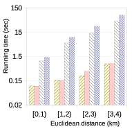
(a) Time budget 400

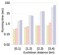
(b) Time budget 600

(c) Time budget 800

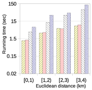
(d) Time budget 1000

Figure 6: Runtime

Search space: We investigate the sizes of search spaces that different methods explore. In particular, we define the search space as the edges that have been explored by a method.

We compare the search spaces that are explored by different methods. Figure 7 shows that the search space of BA is much higher than that of SP in all settings, which is consistent with the performance of runtime shown in Figure 6.

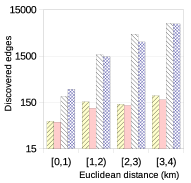
(a) Time budget 400

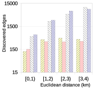
(b) Time budget 600

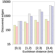
(c) Time budget 800

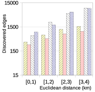
(d) Time budget 1000

Figure 7: Search Space

(a) SP+PACE

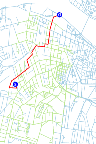
(b) BA+PACE

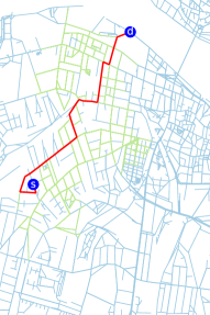
(c) SP+EDGE

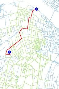
(d) BA+EDGE

Figure 8: A specific $(s,d)$ pair, distance [3, 4), time budget 800

Next, we show visually the edges that are discovered by both heuristic under a specific source-destination pair setting (see the caption of Fig. 8). It is clear that: (1) when using the same model, SP explores much less edges than BA does, indicating the SP heuristic is effective (see the green edges in Fig. 8); (2) the path returned by the PACE model is different from the path returned by the EDGE model (see the red paths in Fig. 8), indicating that the more accurate path distributions captured by PACE do make a difference on the returned paths.

VII Conclusions and Outlook

Arriving on time is an important problem that has many applications in intelligent transportation systems. We present an effective algorithm that solves the SPOTAR problem on the novel path-centric PACE model that considers the dependencies among travel times on different edges. Experimental results on real-world trajectories suggest that the proposed algorithm is effective. In the future, we plan to study further speed-up strategies, e.g., using contraction hierarchies and hub labeling, on top of the PACE model, also possibly using parallel computing [17].

References

- [1] C. Guo, C. S. Jensen, and B. Yang, “Towards Total Traffic Awareness,” SIGMOD Record, vol. 43, no. 3, pp. 18–23, 2014.
- [2] J. Dai, B. Yang, C Guo, C. S. Jensen, and J. Hu, “Path Cost Distribution Estimation Using Trajectory Data,” PVLDB 10(3): 85-96, 2016.
- [3] B. Yang, J. Dai, C Guo, C. S. Jensen, and J. Hu, “PACE: a PAth-CEntric paradigm for stochastic path finding,” VLDB Journal 27(2): 153-178, 2018.
- [4] M. Niknami, S. Samaranayake, “Tractable Pathfinding for the Stochastic On-Time Arrival Problem,” SEA, 231-245, 2016
- [5] G. Sabran, S. Samaranayake, A. Bayen, “Precomputation techniques for the stochastic on-time arrival problem,” ALENEX, 138-146, 2014.
- [6] Yu Nie and Xing Wu, “Shortest path problem considering on-time arrival probability,” Transportation Research Part B: Methodological, 2009.
- [7] C. Guo, B. Yang, O. Andersen, et al. “EcoSky: Reducing vehicular environmental impact through eco-routing.” ICDE, 1412-1415, 2015.
- [8] B. Yang, C. Guo, C. S. Jensen, et al. “Stochastic skyline route planning under time-varying uncertainty.” ICDE, 136–147, 2014.
- [9] B. Yang, M. Kaul, and C. S. Jensen. “Using incomplete information for complete weight annotation of road networks.” TKDE, 26(5):1267–1279, 2014.
- [10] C. Guo, B. Yang, J. Hu, C. S. Jensen. “Learning to Route with Sparse Trajectory Sets.” ICDE, 12 pages, 2018.
- [11] H. Liu, C. Jin, B. Yang, A. Zhou. “Finding Top-k Optimal Sequenced Routes.” ICDE, 12 pages, 2018.
- [12] H. Liu, C. Jin, B. Yang, A. Zhou. “Finding Top-k Shortest Paths with Diversity.” TKDE, 30(3):488-502, 2018.
- [13] J. Hu, B. Yang, C. Guo, C. S. Jensen. “Risk-aware path selection with time-varying, uncertain travel costs: a time series approach.” The VLDB Journal 27(2):179-200, 2018.
- [14] J. Hu, B. Yang, C. S. Jensen, Y. Ma. “Enabling time-dependent uncertain eco-weights for road networks.” GeoInformatica 21(1):57-88, 2017.
- [15] Z. Ding, B. Yang, R. H. Güting, Y. Li. “Network-Matched Trajectory-Based Moving-Object Database: Models and Applications.” IEEE Trans. Intelligent Transportation Systems 16(4):1918-1928, 2015.
- [16] B. Yang, C. Guo, Y. Ma, and C. S. Jensen. “Toward personalized, context-aware routing.” The VLDB Journal, 24(2):297–318, 2015.
- [17] B. Yang, Q. Ma, W. Qian, A. Zhou. TRUSTER: “TRajectory Data Processing on ClUSTERs.” DASFAA, 768-771, 2009.
- [18] Z. Ding, B. Yang, Y. Chi, L. Guo. “Enabling Smart Transportation Systems: A Parallel Spatio-Temporal Database Approach.” IEEE Trans. Computers 65(5): 1377-1391, 2016.