Efficient Contextualized Representation:
Language Model Pruning for Sequence Labeling

Abstract

Many efforts have been made to facilitate natural language processing tasks with pre-trained language models (LMs), and brought significant improvements to various applications. To fully leverage the nearly unlimited corpora and capture linguistic information of multifarious levels, large-size LMs are required; but for a specific task, only parts of these information are useful. Such large-sized LMs, even in the inference stage, may cause heavy computation workloads, making them too time-consuming for large-scale applications. Here we propose to compress bulky LMs while preserving useful information with regard to a specific task. As different layers of the model keep different information, we develop a layer selection method for model pruning using sparsity-inducing regularization. By introducing the dense connectivity, we can detach any layer without affecting others, and stretch shallow and wide LMs to be deep and narrow. In model training, LMs are learned with layer-wise dropouts for better robustness. Experiments on two benchmark datasets demonstrate the effectiveness of our method.

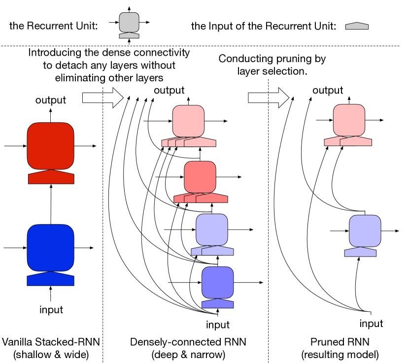
Figure 1: Leverage the dense connectivity to compress models via layer selection, and replace wide and shallow RNNs with deep and narrow ones.

1 Introduction

Benefited from the recent advances in neural networks (NNs) and the access to nearly unlimited corpora, neural language models are able to achieve a good perplexity score and generate high-quality sentences. These LMs automatically capture abundant linguistic information and patterns from large text corpora, and can be applied to facilitate a wide range of NLP applications Rei (2017); Liu et al. (2018); Peters et al. (2018).

Recently, efforts have been made on learning contextualized representations with pre-trained language models (LMs)  Peters et al. (2018). These pre-trained layers brought significant improvements to various NLP benchmarks, yielding up to $30\%$ relative error reductions. However, due to high variability of language, gigantic NNs (e.g., LSTMs with 8,192 hidden states) are preferred to construct informative LMs and extract multifarious linguistic information Peters et al. (2017). Even though these models can be integrated without retraining (using their forward pass only), they still result in heavy computation workloads during inference stage, making them prohibitive for real-world applications.

In this paper, we aim to compress LMs for the end task in a plug-in-and-play manner. Typically, NN compression methods require the retraining of the whole model Mellempudi et al. (2017). However, neural language models are usually composed of RNNs, and their backpropagations require significantly more RAM than their inference. It would become even more cumbersome when the target task equips the coupled LMs to capture information in both directions. Therefore, these methods do not fit our scenario very well. Accordingly, we try to compress LMs while avoiding costly retraining.

Intuitively, layers of different depths would capture linguistic information of different levels. Meanwhile, since LMs are trained in a task-agnostic manner, not all layers and their extracted information are relevant to the end task. Hence, we propose to compress the model by layer selection, which retains useful layers for the target task and prunes irrelevant ones. However, for the widely-used stacked-LSTM, directly pruning any layers will eliminate all subsequent ones. To overcome this challenge, we introduce the dense connectivity. As shown in Fig. 1, it allows us to detach any layers while keeping all remaining ones, thus creating the basis to avoid retraining. Moreover, such connectivity can stretch shallow and wide LMs to be deep and narrow Huang et al. (2017), and enable a more fine-grained layer selection.

Furthermore, we try to retain the effectiveness of the pruned model. Specifically, we modify the $L_{1}$ regularization for encouraging the selection weights to be not only sparse but binary, which protects the retained layer connections from shrinkage. Besides, we design a layer-wise dropout to make LMs more robust and better prepared for the layer selection.

We refer to our model as LD-Net, since the layer selection and the dense connectivity form the basis of our pruning methods. For evaluation, we apply LD-Net on two sequence labeling benchmark datasets, and demonstrated the effectiveness of the proposed method. In the CoNLL03 Named Entity Recognition (NER) task, the $F_{1}$ score increases from 90.78$\pm$0.24% to 91.86$\pm$0.15% by integrating the unpruned LMs. Meanwhile, after pruning over 90% calculation workloads from the best performing model (92.03%), the resulting model still yields 91.84$\pm$0.14%. Our implementations and pre-trained models would be released for futher study.

2 LD-Net

Given a input sequence of $T$ word-level tokens, $\{x_{1}$, $x_{2}$, $\cdots$, $x_{T}\}$, we use $\mathbf{x}_{t}$ to denote the embedding of $x_{t}$. For a $L$-layers NN, we mark the input and output of the $l^{th}$ layer at the $t^{th}$ time stamp as $\mathbf{x}_{l,t}$ and $\mathbf{h}_{l,t}$.

2.1 RNN and Dense Connectivity

We represent one RNN layer as a function:

$$\mathbf{h}_{l,t}=F_{l}(\mathbf{x}_{l,t},\mathbf{h}_{l,t-1})$$ (1)

where $F_{l}$ is the recurrent unit of $l^{th}$ layer, it could be any RNNs variants, and the vanilla LSTMs is used in our experiments.

As deeper NNs usually have more representation power, RNN layers are often stacked together to form the final model by setting $\mathbf{x}_{l,t}=\mathbf{h}_{l-1,t}$. These vanilla stacked-RNN models, however, suffer from problems like the vanishing gradient, and it’s hard to train very deep models.

Recently, the dense connectivity and residual connectivity have been proposed to handle these problems He et al. (2016); Huang et al. (2017). Specifically, dense connectivity refers to adding direct connections from any layer to all its subsequent layers. As illustrated in Figure 1, the input of $l^{th}$ layer is composed of the original input and the output of all preceding layers as follows.

$$\mathbf{x}_{l,t}=[\mathbf{x}_{t},\mathbf{h}_{1,t},\cdots,\mathbf{h}_{l-1,t}]$$

Similarly, the final output of the $L$-layer RNN is $\mathbf{h}_{t}=[\mathbf{x}_{t},\mathbf{h}_{1,t},\cdots,\mathbf{h}_{L,t}]$. With dense connectivity, we can detach any single layer without eliminating its subsequent layers (as in Fig. 1). Also, existing practices in computer vision demonstrate that such connectivities can lead to deep and narrow NNs and distribute parameters into different layers. Moreover, different layers in LMs usually capture linguistic information of different levels. Hence, we can compress LMs for a specific task by pruning unrelated or unimportant layers.

2.2 Language Modeling

Language modeling aims to describe the sequence generation. Normally, the generation probability of the sequence $\{x_{1},\cdots,x_{T}\}$ is defined in a “forward” manner:

$$p(x_{1},\cdots,x_{T})=\prod_{t=1}^{T}p(x_{t}|x_{1},\cdots,x_{t-1})$$ (2)

Where $p(x_{t}|x_{1},\cdots,x_{t-1})$ is computed based on the output of RNN, $\mathbf{h}_{t}$. Due to the dense connectivity, $\mathbf{h}_{t}$ is composed of outputs from different layers, which are designed to capture linguistic information of different levels. Similar to the bottleneck layers employed in the DenseNet Huang et al. (2017), we add additional layers to unify such information. Accordingly, we add an projection layer with the $\mathrm{ReLU}$ activation function:

$$\mathbf{h}_{t}^{*}=\mathrm{ReLU}(W_{proj}\cdot\mathbf{h}_{t}+\mathbf{b}_{proj})$$ (3)

Based on $\mathbf{h}_{t}^{*}$, it’s intuitive to calculate $p(x_{t}|x_{1},\cdots,x_{t-1})$ by the softmax function, i.e., $\mathrm{softmax}(W_{out}\cdot\mathbf{h}_{t}^{*}+\mathbf{b})$.

Since the training of language models needs nothing but the raw text, it has almost unlimited corpora. However, conducting training on extensive corpora results in a huge dictionary, and makes calculating the vanilla softmax intractable. Several techniques have been proposed to handle this problem, including adaptive softmax Grave et al. (2017), slim word embedding Li et al. (2018), the sampled softmax and the noise contrastive estimation Józefowicz et al. (2016). Since the major focus of our paper does not lie in the language modeling task, we choose the adaptive softmax because of its practical efficiency when accelerated with GPUs.

2.3 Contextualized Representations

As pre-trained LMs can describe the text generation accurately, they can be utilized to extract information and construct features for other tasks. These features, referred as contextualized representations, have been demonstrated to be essentially useful Peters et al. (2018). To capture information from both directions, we utilized not only forward LMs, but also backward LMs. Backward LMs are based on Eqn. 4 instead of Eqn. 2. Similar to forward LMs, backward LMs approach $p(x_{t}|x_{t+1},\cdots,x_{T})$ with NNs. For reference, the output of the RNN in backward LMs for $x_{t}$ is recorded as $\mathbf{h}_{t}^{r}$.

$$p(x_{1},\cdots,x_{n})=\prod_{t=1}^{T}p(x_{t}|x_{t+1},\cdots,x_{T})$$ (4)

Ideally, the final output of LMs (e.g., $\mathbf{h}_{t}^{*}$) would be the same as the representation of the target word (e.g., $x_{t+1}$); therefore, it may not contain much context information. Meanwhile, the output of the densely connected RNN (e.g., $\mathbf{h}_{t}$) includes outputs from every layer, thus summarizing all extracted features. Since the dimensions of $\mathbf{h}_{t}$ could be too large for the end task, we add a non-linear transformation to calculate the contextualized representation ($\mathbf{r}_{t}$):

$$\mathbf{r}_{t}=\mathrm{ReLU}(W_{cr}\cdot[\mathbf{h}_{t},\mathbf{h}_{t}^{r}]+\mathbf{b}_{cr})$$ (5)

Our proposed method bears the same intuition as the ELMo Peters et al. (2018). ELMo is designed for the vanilla stacked-RNN, and tries to calculate a weighted average of different layers’ outputs as the contextualized representation. Our method, benefited from the dense connectivity and its narrow structure, can directly combine the outputs of different layers by concatenation. It does not assume the outputs of different layers to be in the same vector space, thus having more potential for transferring the constructed token representations. More discussions are available in Sec. 4.

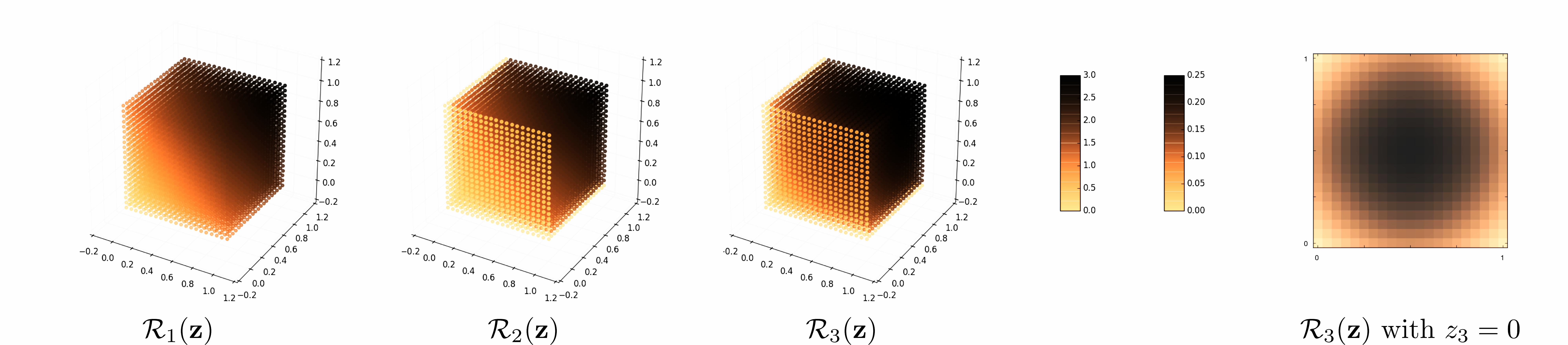
Figure 2: Penalty values of various $\mathcal{R}$ for $\mathbf{z}$ with three dimensions. $\lambda_{1}$ has been set to $2$ for $\mathcal{R}_{2}$ and $\mathcal{R}_{3}$.

2.4 Layer Selection

Typical model compression methods require retraining or gradient calculation. For the coupled LMs, these methods require even more computation resources compared to the training of LMs, thus not fitting our scenario very well.

Benefited from the dense connectivity, we are able to train deep and narrow networks. Moreover, we can detach one of its layer without eliminating all subsequent layers (as in Fig. 1). Since different layers in NNs could capture different linguistic information, only a few of them would be relevant or useful for a specific task. As a result, we try to compress these models by the task-guided layer selection. For $i$-th layer, we introduce a binary mask $z_{i}\in\{0,1\}$ and calculate $\mathbf{h}_{l,t}$ with Eqn. 6 instead of Eqn. 1.

$$\mathbf{h}_{l,t}=z_{i}\cdot F_{l}(\mathbf{x}_{l,t},\mathbf{h}_{l,t-1})$$ (6)

With this setting, we can conduct a layer selection by optimizing the regularized empirical risk:

$$\min\mathcal{L}+\lambda_{0}\cdot\mathcal{R}$$ (7)

where $\mathcal{L}$ is the empirical risk for the sequence labeling task and $\mathcal{R}$ is the sparse regularization.

The ideal choice for $\mathcal{R}$ would be the $L_{0}$ regularization of $\mathbf{z}$, i.e., $\mathcal{R}_{0}(\mathbf{z})=|\mathbf{z}|_{0}$. However, it is not continuous and cannot be efficiently optimized. Hence, we relax $z_{i}$ from binary to a real value (i.e., $0\leq z_{i}\leq 1$) and replace $\mathcal{R}_{0}$ by:

$$\mathcal{R}_{1}=|\mathbf{z}|_{1}$$

Despite the sparsity achieved by $\mathcal{R}_{1}$, it could hurt the performance by shifting all $z_{i}$ far away from $1$. Such shrinkage introduces additional noise in $\mathbf{h}_{l,t}$ and $\mathbf{x}_{l,t}$, which may result in ineffective pruned LMs. Since our goal is to conduct pruning without retraining, we further modify the $L_{1}$ regularization to achieve sparsity while alleviating its shrinkage effect. As the target of $\mathcal{R}$ is to make $\mathbf{z}$ sparse, it can be “turned-off” after achieving a satisfying sparsity. Therefore, we extend $\mathcal{R}_{1}$ to a margin-based regularization:

$$\mathcal{R}_{2}=\delta(|\mathbf{z}|_{0}>\lambda_{1})|\mathbf{z}|_{1}$$

In addition, we also want to make up the relaxation made on $\mathbf{z}$, i.e., relaxing its values from binary to $[0,1]$. Accordingly, we add the penalty $|\mathbf{z}(1-\mathbf{z})|_{1}$ to encourage $\mathbf{z}$ to be binary Murray and Ng (2010) and modify $\mathcal{R}_{2}$ into $\mathcal{R}_{3}$:

$$\mathcal{R}_{3}=\delta(|\mathbf{z}|_{0}>\lambda_{1})|\mathbf{z}|_{1}+|\mathbf{z}(1-\mathbf{z})|_{1}$$

To compare $\mathcal{R}_{1}$, $\mathcal{R}_{2}$ and $\mathcal{R}_{3}$, we visualize their penalty values in Fig. 2. The visualization is generated for a $3$-dimensional $\mathbf{z}$ while the targeted sparsity, $\lambda_{1}$, is set to $2$. Comparing to $\mathcal{R}_{1}$, we can observe that $\mathcal{R}_{2}$ enlarges the optimal point set from $\mathbf{0}$ to all $\mathbf{z}$ with a satisfying sparsity, thus avoiding the over-shrinkage. To better demonstrate the effect of $\mathcal{R}_{3}$, we further visualize its penalties after achieving a satisfying sparsity (w.l.o.g., assuming $z_{3}=0$). One can observe that it penalizes non-binary $\mathbf{z}$ and favors binary values.

2.5 Layer-wise Dropout

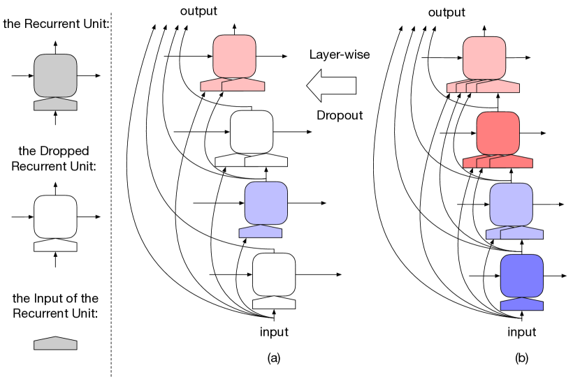
Figure 3: Layer-wise dropout conducted on a 4-layer densely connected RNN. (a) is the remained RNN. (b) is the original densely connected RNN.

So far, we’ve customized the regularization term for the layer-wise pruning, which protects the retained connections among layers from shrinking. After that, we try to further retain the effectiveness of the compressed model. Specifically, we choose to prepare the LMs for the pruned inputs, thus making them more robust to pruning.

Accordingly, we conduct the training of LMs with a layer-wise dropout. As in Figure 3, a random part of layers in the LMs are randomly dropped during each batch. The outputs of the dropped layers will not be passed to their subsequent recurrent layers, but will be sent to the projection layer (Eqn. 3) for predicting the next word. In other words, this dropout is only applied to the input of recurrent layers, which aims to imitate the pruned input without totally removing any layers.

3 Sequence Labeling

In this section, we will introduce our sequence labeling architecture, which is augmented with the contextualized representations.

3.1 Neural Architecture

Following the recent studies Liu et al. (2018); Kuru et al. (2016), we construct the neural architecture as in Fig. 4. Given the input sequence $\{x_{1},x_{2},\cdots,x_{T}\}$, for $t^{th}$ token ($x_{t}$), we assume its word embedding is $\mathbf{w}_{t}$, its label is $y_{t}$, and its character-level input is $\{c_{i,1},c_{i,2},\cdots,c_{i,\_}\}$, where $c_{i,\_}$ is the space character following $x_{t}$.

The character-level representations have become the required components for most of the state-of-the-art. Following the recent study Liu et al. (2018), we employ LSTMs to take the character-level input in a context-aware manner, and mark its output for $x_{t}$ as $\mathbf{c}_{t}$. Similar to the contextualized representation, $\mathbf{c}_{t}$ usually has more dimensions than $\mathbf{w}_{t}$. To integrate them together, we set the output dimension of Eqn. 5 as the dimension of $\mathbf{w}_{t}$, and project $\mathbf{c}_{t}$ to a new space with the same dimension number. We mark the projected character-level representation as $\mathbf{c}_{t}^{*}$.

After projections, these vectors are concatenated as $\mathbf{v}_{t}=[\mathbf{c}_{t}^{*};\mathbf{r}_{t};\mathbf{w}_{t}],\forall i\in[1,T]$ and further fed into the word-level LSTMs. We refer to their output as $\mathbf{U}=\{\mathbf{u}_{1},\cdots,\mathbf{u}_{T}\}$. To ensure the model to predict valid label sequences, we append a first-order conditional random field (CRF) layer to the model Lample et al. (2016). Specifically, the model defines the generation probability of $\mathbf{y}=\{y_{1},\cdots,y_{T}\}$ as

$$p(\mathbf{y}|\mathbf{U})=\frac{\prod_{t=1}^{T}\phi(y_{t-1},y_{t},\mathbf{u}_{t})}{\sum_{\hat{\mathbf{y}}\in\mathbf{Y}(\mathbf{U})}\prod_{t=1}^{T}\phi(\hat{y}_{t-1},\hat{y}_{t},\mathbf{u}_{t})}$$ (8)

where $\hat{\mathbf{y}}=\{\hat{y}_{1},\dots,\hat{y}_{T}\}$ is a generic label sequence, $\mathbf{Y}(\mathbf{U})$ is the set of all generic label sequences for $\mathbf{U}$ and $\phi(y_{t-1},y_{t},\mathbf{u}_{t})$ is the potential function. In our model, $\phi(y_{t-1},y_{t},\mathbf{u}_{t})$ is defined as $\exp(W_{y_{t}}\mathbf{u}_{t}+b_{y_{t-1},y_{t}})$, where $W_{y_{t}}$ and $b_{y_{t-1},y_{t}}$ are the weight and bias parameters.

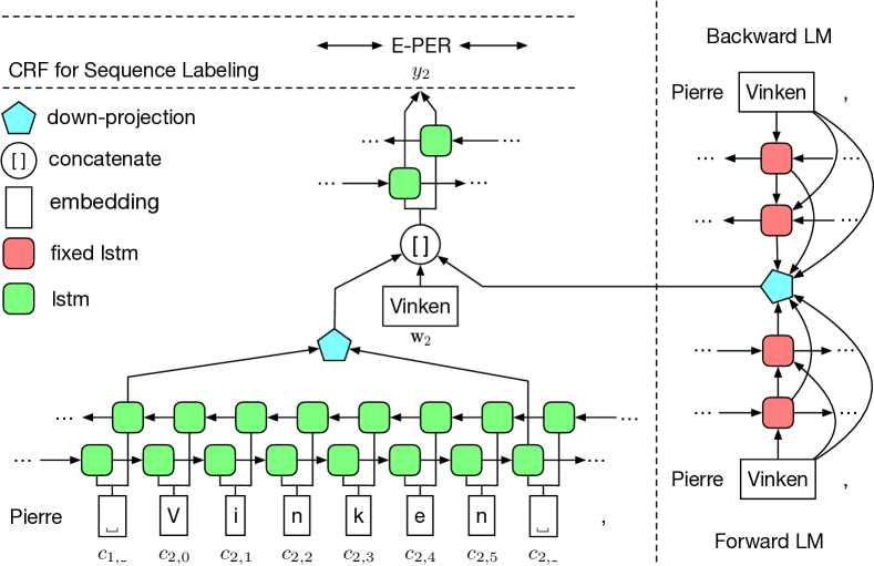
Figure 4: The proposed sequence labeling architecture with contextualized representations.

3.2 Model Training and Inference

We use the following negative log-likelihood as the empirical risk.

$$\mathcal{L}=-\sum_{\mathbf{U}}\log p(\mathbf{y}|\mathbf{U})$$ (9)

For testing or decoding, we want to find the optimal sequence $\mathbf{y}^{*}$ that maximizes the likelihood.

$$\mathbf{y}^{*}=\underset{\mathbf{y}\in\mathbf{Y}(\mathbf{U})}{{\mbox{argmax}}}\;p(\mathbf{y}|\mathbf{U})$$ (10)

Although the denominator of Eq. 8 is complicated, we can calculate Eqs. 9 and 10 efficiently by the Viterbi algorithm.

For optimization, we decompose it into two steps, i.e., model training and model pruning.

Model training. We set $\lambda_{0}$ to $0$ and optimize the empirical risk without any regularization, i.e., $\min\mathcal{L}$. In this step, we conduct optimization with the stochastic gradient descent with momentum. Following Peters et al. (2018), dropout would be added to both the coupled LMs and the sequence labeling model.

Model pruning. We conduct the pruning based on the checkpoint which has the best performance on the development set during the model training. We set $\lambda_{0}$ to non-zero values and optimize $\min\mathcal{L}+\lambda_{0}\mathcal{R}_{3}$ by the projected gradient descent with momentum. Any layer $i$ with $z_{i}=0$ would be deleted in the final model to complete the pruning. To get a better stability, dropout is only added to the sequence labeling model.

Network	Ind. #	Hid. #	Layer #	Param.# ($\cdot 10^{7}$)		PPL
				RNN	Others
8192-1024 Józefowicz et al. (2016)	1	8192	2	15.1♯	163♯	30.6
CNN-8192-1024 Józefowicz et al. (2016)	2	8192	2	15.1♯	89♯	30.0
CNN-4096-512 Peters et al. (2018)	3	4096	2	3.8♯	40.6♯	39.7
2048-512 Peters et al. (2017)	4	2048	1	0.9♯	40.6♯	47.50
2048-Adaptive Grave et al. (2017)	5	2048	2	5.2†	26.5†	39.8
vanilla LSTM	6	2048	2	5.3†	25.6†	40.27
	7	1600	2	3.2†	24.2†	48.85
LD-Net without Layer-wise Dropout	8	300	10	2.3†	24.2†	45.14
LD-Net with Layer-wise Dropout	9	300	10	2.3†	24.2†	50.06

Table 1: Performance comparison of language models. Models marked with^† adopted adaptive softmax and the vanilla LSTMs, which has less softmax parameters. Models marked with^♯ employed sampled softmax LSTMs w. projection, which results in less RNN parameters w.r.t. the size of hidden states.

4 Experiments

We will first discuss the capability of the LD-Net as language models, then explore the effectiveness of its contextualized representations.

4.1 Language Modeling

For comparison, we conducted experiments on the one billion word benchmark dataset Chelba et al. (2013) with both LD-Net (with 1,600 dimensional projection) and the vanilla stacked-LSTM. Both kinds of models use word embedding (random initialized) of 300 dimension as input and use the adaptive softmax (with default setting) as an approximation of the full softmax. Additionally, as preprocessing, we replace all tokens occurring equal or less than 3 times with as UNK, which shrinks the dictionary from 0.79M to 0.64M.

The optimization is performed by the Adam algorithm Kingma and Ba (2014), the gradient is clipped at $5.0$ and the learning rate is set to start from $0.001$. The layer-wise dropout ratio is set to $0.5$, the RNNs are unrolled for 20 steps without resetting the LSTM states, and the batch size is set to 128. Their performances are summarized in Table 1, together with several LMs used in our sequence labeling baselines. For models without official reported parameter numbers, we estimate their values (marked with^†) by assuming they adopted the vanilla LSTM. Note that, for models 3, 5, 6, 7, 8, and 9, PPL refers to the averaged perplexity of the forward and the backward LMs.

We can observe that, for those models taking word embedding as the input, embedding composes the vast majority of model parameters. However, embedding can be embodied as a “sparse” layer which is computationally efficient. Instead, the intense calculations are conducted in RNN layers and softmax layer for language modeling, or RNN layers for contextualized representations. At the same time, comparing the model 8192-1024 and CNN-8192-1024, their only difference is the input method. Instead of taking word embedding as the input, CNN-8192-1024 utilizes CNN to compose word representation from the character-level input. Despite the greatly reduced parameter number, the perplexity of the resulting models remains almost unchanged. Since replacing embedding layer with CNN would make the training slower, we only conduct experiments with models taking word embedding as the input.

Comparing LD-Net with other baselines, we think it achieves satisfactory performance with regard to the size of hidden states. It demonstrates the LD-Net’s capability of capturing the underlying structure of natural language. Meanwhile, we find that the layer-wise dropout makes it harder to train LD-Net and its resulting model achieves less competitive results. However, as would be discussed in the next section, layer-wise dropout allows the resulting model to generate better contextualized representations and be more robust to pruning, even with a higher perplexity.

4.2 Sequence Labeling

Following TagLM Peters et al. (2017), we evaluate our methods in two benchmark datasets, the CoNLL03 NER task Tjong Kim Sang and De Meulder (2003) and the CoNLL00 Chunking task Tjong Kim Sang and Buchholz (2000).

CoNLL03 NER has four entity types and includes the standard training, development and test sets.

CoNLL00 chunking defines eleven syntactic chunk types (e.g., NP and VP) in addition to Other. Since it only includes training and test sets, we sampled 1000 sentences from training set as a held-out development set Peters et al. (2017).

In both cases, we use the BIOES labeling scheme Ratinov and Roth (2009) and use the micro-averaged $F_{1}$ as the evaluation metric. Based on the analysis conducted in the development set, we set $\lambda_{0}=0.05$ for the NER task, and $\lambda_{0}=0.5$ for the Chunking task. As discussed before, we conduct optimization with the stochastic gradient descent with momentum. We set the batch size, the momentum, and the learning rate to $10$, $0.9$, and $\eta_{t}=\frac{\eta_{0}}{1+\rho t}$ respectively. Here, $\eta_{0}=0.015$ is the initial learning rate and $\rho=0.05$ is the decay ratio. Dropout is applied in our model, and its ratio is set to $0.5$. For a better stability, we use gradient clipping of $5.0$. Furthermore, we employ the early stopping in the development set and report averaged score across five different runs.

Regarding the network structure, we use the 30-dimension character-level embedding. Both character-level and word-level RNNs are set to one-layer LSTMs with 150-dimension hidden states in each direction. The GloVe 100-dimension pre-trained word embedding is used as the initialization of word embedding $\mathbf{w}_{t}$, and will be fine-tuned during the training. The layer selection variables $z_{i}$ are initialized as $1$, remained unchanged during the model training and only be updated during the model pruning. All other variables are randomly initialized Glorot and Bengio (2010).

Network	Avg.	#FLOPs	$F_{1}$ score
(LMs Ind.#)	ppl	($\cdot 10^{6}$)	(avg$\pm$std)
NoLM (/)	/	3	94.42$\pm$0.08
R-ELMo (6)	40.27	108	96.19$\pm$0.07
R-ELMo (7)	48.85	68	95.86$\pm$0.04
LD-Net ∗ (8)	45.14	51	96.01$\pm$0.07
LD-Net ∗ (9)	50.06	51	96.05$\pm$0.08
LD-Net (8)	origin	51	96.13
	pruned	13	95.46$\pm$0.18
LD-Net (9)	origin	51	96.15
	pruned	10	95.66$\pm$0.04

Table 2: Performance comparisons in the CoNLL00 Chunking task. LD-Net maked with ^∗ are trained without pruning (layer selection).

Network	Avg.	#FLOPs	$F_{1}$ score
(LMs Ind.#)	ppl	($\cdot 10^{6}$)	(avg$\pm$std)
NoLM (/)	/	3	90.78$\pm$0.24
O-ELMo (3)	39.70	79♯	92.22$\pm$0.10
TagLM (4)	47.50	22♯	91.62$\pm$0.23
R-ELMo (6)	40.27	108	91.99$\pm$0.24
R-ELMo (7)	48.85	68	91.54$\pm$0.10
LD-Net ∗ (8)	45.14	98	91.76$\pm$0.18
LD-Net ∗ (9)	50.06	98	91.86$\pm$0.15
LD-Net (8)	origin	51	91.95
	pruned	5	91.55$\pm$0.06
LD-Net (9)	origin	51	92.03
	pruned	5	91.84$\pm$0.14

Table 3: Performance comparison in the CoNLL03 NER task. Models marked with^† employed LSTMs with projection, which is more efficient than the vanilla LSTMs. LD-Net maked with ^∗ are trained without pruning (layer selection).

Network (LMs Ind.#)	FLOPs	Batch size	Peak RAM	Time (s)	Speed
					$10^{3}$words/s	$10^{3}$sents/s
R-ELMo (6)	108	200	8Gb	32.88	22	0.4
LD-Net (9, origin)	51	80	8Gb	25.68	26	0.5
LD-Net (9, pruned)	5	80	4Gb	6.90	98	2.0
		500	8Gb	4.86 (5X)	166 (6X)	2.9 (5X)

Table 4: Speed comparison in the CoNLL03 NER task. We can observe that LD-Net (9, pruned) achieved about 5 times speed up on the wall-clock time over LD-Net (9, origin).

Compared methods. The first baseline, referred as NoLM, is our sequence labeling model without the contextualized representations, i.e., calculating $\mathbf{v}_{t}$ as $[\mathbf{c}_{t}^{*};\mathbf{w}_{t}]$ instead of $[\mathbf{c}_{t}^{*};\mathbf{r}_{t};\mathbf{w}_{t}]$. Besides, ELMo Peters et al. (2018) is the major baseline. To make comparison more fair, we implemented the ELMo model and use it to calculate the $\mathbf{r}_{t}$ in Eqn. 5 instead of $[\mathbf{h}_{t},\mathbf{h}_{t}^{r}]$. Results of re-implemented models are referred with R-ELMo ($\lambda$ is set to the recommended value, $0.1$) and the results reported in its original paper are referred with O-ELMo. Additionally, since TagLM Peters et al. (2017) with one-layer NNs can be viewed as a special case of ELMo, we also include its results.

Sequence labeling results. Table 2 and  3 summarizes the results of LD-Net and baselines. Besides the $F_{1}$ score and averaged perplexity, we also estimate FLOPs (i.e., the number of floating-point multiplication-adds) for the efficiency evaluation. Since our model takes both word-level and character-level inputs, we estimated the FLOPs value for a word-level input with $4.39$ character-level inputs, while $4.39$ is the averaged length of words in the CoNLL03 dataset.

Before the model pruning, LD-Net achieves a 96.05$\pm$0.08 $F_{1}$ score in the CoNLL00 Chunking task, yielding nearly 30% error reductions over the NoLM baseline. Also, it scores 91.86$\pm$0.15 $F_{1}$ in the CoNLL03 NER task with over 10% error reductions. Similar to the language modeling, we observe that the most complicated models achieve the best perplexity and provide the most improvements in the target task. Still, considering the number of model parameters and the resulting perplexity, our model demonstrates its effectiveness in generating contextualized representations. For example, comparing to our methods, R-ELMo (7) leverages LMs with the similar perplexity and parameter number, but cannot get the same improvements with our method on both datasets.

Actually, contextualized representations have strong connections with the skip-thought vectors Kiros et al. (2015). Skip-thought models try to embed sentences and are trained by predicting the previous and afterwards sentences. Similarly, LMs encode a specific context as the hidden states of RNNs, and use them to predict future contexts. Specifically, we recognize the cell states of LSTMs are more like to be the sentence embedding Radford et al. (2017), since they are only passed to the next time stamps. At the same time, because the hidden states would be passed to other layers, we think they are more like to be the token representations capturing necessary signals for predicting the next word or updating context representations. Hence, LD-Net should be more effective then ELMo, as concatenating could preserve all extracted signals while weighted average might cause information loss.

Although the layer-wise dropout makes the model harder to train, their resulting LMs generate better contextualized representations, even without the same perplexity. Also, as discussed in Peters et al. (2018, 2017), the performance of the contextualized representation can be further improved by training larger models or using the CNN to represent words.

For the pruning, we started from the model with the best performance on the development set (referred with “origin”), and refer the performances of pruned models with “pruned” in Table 2 and  3. Essentially, we can observe the pruned models get rid of the vast majority of calculation while still retaining a significant improvement. We will discuss more on the pruned models in Sec. 4.4.

4.3 Speed Up Measurements

We use FLOPs for measuring the inference efficiency as it reflects the time complexity Han et al. (2015), and thus is independent of specific implementations. For models with the same structure, improvements in FLOPs would result in monotonically decreasing inference time. However, it may not reflect the actual efficiency of models due to the model differences in parallelism. Accordingly, we also tested wall-clock speeds of our implementations.

Our implementations are based on the PyTorch 0.3.1, and all experiments are conducted on the CoNLL03 dataset with the Nvidia GTX 1080 GPU. Specifically, due to the limited size of CoNLL03 test set, we measure such speeds on the training set. As in Table 4, we can observe that, the pruned model achieved about 5 times speed up. Although there is still a large margin between the actual speed-up and the FLOPs speed-up, we think the resulting decode speed (166K words/s) is sufficient for most real-world applications.

4.4 Case Studies

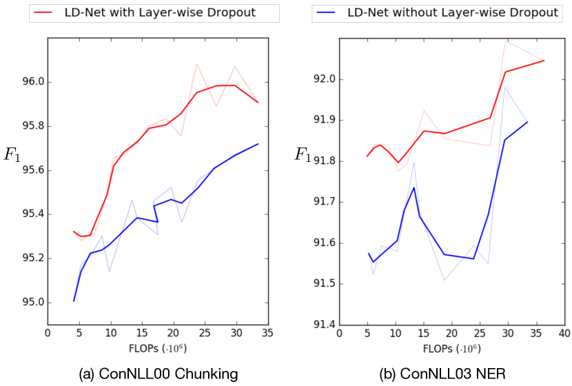
Figure 5: The performance of pruned models in two tasks w.r.t. their efficiency (FLOPs).

Effect of the pruning ratio. To explore the effect of the pruning ratio, we adjust $\lambda_{1}$ and visualize the performance of pruned models v.s. their FLOPs # in Fig 5. We can observe that LD-Net outperforms its variants and demonstrates its effectiveness.

As the pruning ratio becoming larger, we can observe the performance of LD-Net first increases a little, then starts dropping. Besides, in the CoNLL03 NER task, LMs can be pruned to a relatively small size without much loss of efficiency. As in Table 3, we can observe that, after pruning over 90% calculations, the error of the resulting model only increases about 2%, yielding a competitive performance. As for the CoNLL00 Chunking task, the performance of LD-Net decays in a faster rate than that in the NER task. For example, after pruning over 80% calculations, the error of the resulting model increases about 13%. Considering the fact that this corpus is only half the size of the CoNLL03 NER dataset, we can expect the resulting models have more dependencies on the LMs. Still, the pruned model achieves a 25% error reduction over the NoLM baseline.

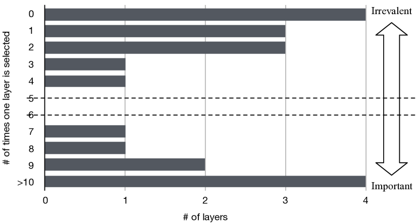
Figure 6: The performance of pruned models in two tasks w.r.t. their efficiency (FLOPs).

Layer selection pattern. We further studied the layer selection patterns. Specifically, we use the same setting of LD-Net (9) in Table 3, conduct model pruning using for 50 times, and summarize the statics in Figure 6. We can observe that network layers formulate two clear clusters, one is likely to be preserved during the selection, and the other is likely to be pruned. This is consistent with our intuition that some layers are more important than others and the layer selection algorithm would pick up layers meaningfully.

However, there is some randomness in the selection result. We conjugate that large networks trained with dropout can be viewed as a ensemble of small sub-networks Hara et al. (2016), also there would be several sub-networks having the similar function. Accordingly, we think the randomness mainly comes from such redundancy.

Effectiveness of model pruning. Zhu and Gupta (2017) observed pruned large models consistently outperform small models on various tasks (including LM). These observations are consistent with our experiments. For example, LD-Net achieves 91.84 after pruning on the CoNLL03 dataset. It outperforms TagLM (4) and R-ELMo (7), whose performances are $91.62$ and $91.54$. Besides, we trained small LMs of the same size as the pruned LMs (1-layer densely connected LSTMs). Its perplexity is 69 and its performance on the CoNLL03 dataset is $91.55\pm 0.19$.

5 Related Work

Sequence labeling. Linguistic sequence labeling is one of the fundamental tasks in NLP, encompassing various applications including POS tagging, chunking, and NER. Many attempts have been made to conduct end-to-end learning and build reliable models without handcrafted features Chiu and Nichols (2016); Lample et al. (2016); Ma and Hovy (2016).

Language modeling. Language modeling is a core task in NLP. Many attempts have been paid to develop better neural language models Zilly et al. (2017); Inan et al. (2016); Godin et al. (2017); Melis et al. (2017). Specifically, with extensive corpora, language models can be well trained to generate high-quality sentences from scratch Józefowicz et al. (2016); Grave et al. (2017); Li et al. (2018); Shazeer et al. (2017). Meanwhile, initial attempts have been made to improve the performance of other tasks with these methods. Some methods treat the language modeling as an additional supervision, and conduct co-training for knowledge transfer Dai and Le (2015); Liu et al. (2018); Rei (2017). Others, including this paper, aim to construct additional features (referred as contextualized representations) with the pre-trained language models Peters et al. (2017, 2018).

Neural Network Acceleration. There are mainly three kinds of NN acceleration methods, i.e., prune network into smaller sizes Han et al. (2015); Wen et al. (2016), converting float operation into customized low precision arithmetic Hubara et al. (2018); Courbariaux et al. (2016), and using shallower networks to mimic the output of deeper ones Hinton et al. (2015); Romero et al. (2014). However, most of them require costly retraining.

6 Conclusion

Here, we proposed LD-Net, a novel framework for efficient contextualized representation. As demonstrated on two benchmarks, it can conduct the layer-wise pruning for a specific task. Moreover, it requires neither the gradient oracle of LMs nor the costly retraining. In the future, we plan to apply LD-Net to other applications.

References

- Chelba et al. (2013) Ciprian Chelba, Tomas Mikolov, Mike Schuster, Qi Ge, Thorsten Brants, Phillipp Koehn, and Tony Robinson. 2013. One billion word benchmark for measuring progress in statistical language modeling. Technical report, Google.
- Chiu and Nichols (2016) Jason P. C. Chiu and Eric Nichols. 2016. Named entity recognition with bidirectional lstm-cnns. TACL.
- Courbariaux et al. (2016) Matthieu Courbariaux, Itay Hubara, Daniel Soudry, Ran El-Yaniv, and Yoshua Bengio. 2016. Binarized neural networks: Training deep neural networks with weights and activations constrained to+ 1 or-1. arXiv preprint arXiv:1602.02830.
- Dai and Le (2015) Andrew M Dai and Quoc V Le. 2015. Semi-supervised sequence learning. In Advances in neural information processing systems, pages 3079–3087.
- Glorot and Bengio (2010) Xavier Glorot and Yoshua Bengio. 2010. Understanding the difficulty of training deep feedforward neural networks. In Proceedings of the Thirteenth International Conference on Artificial Intelligence and Statistics.
- Godin et al. (2017) Fréderic Godin, Joni Dambre, and Wesley De Neve. 2017. Improving language modeling using densely connected recurrent neural networks. arXiv preprint arXiv:1707.06130.
- Grave et al. (2017) Edouard Grave, Armand Joulin, Moustapha Cissé, David Grangier, and Hervé Jégou. 2017. Efficient softmax approximation for gpus. In International Conference on Machine Learning, pages 1302–1310.
- Han et al. (2015) Song Han, Jeff Pool, John Tran, and William Dally. 2015. Learning both weights and connections for efficient neural network. In Advances in neural information processing systems, pages 1135–1143.
- Hara et al. (2016) Kazuyuki Hara, Daisuke Saitoh, and Hayaru Shouno. 2016. Analysis of dropout learning regarded as ensemble learning. In International Conference on Artificial Neural Networks, pages 72–79. Springer.
- He et al. (2016) Kaiming He, Xiangyu Zhang, Shaoqing Ren, and Jian Sun. 2016. Identity mappings in deep residual networks. In European Conference on Computer Vision, pages 630–645. Springer.
- Hinton et al. (2015) Geoffrey E. Hinton, Oriol Vinyals, and Jeffrey Dean. 2015. Distilling the knowledge in a neural network. CoRR, abs/1503.02531.
- Huang et al. (2017) Gao Huang, Zhuang Liu, Laurens Van Der Maaten, and Kilian Q Weinberger. 2017. Densely connected convolutional networks. In CVPR.
- Hubara et al. (2018) Itay Hubara, Matthieu Courbariaux, Daniel Soudry, Ran El-Yaniv, and Yoshua Bengio. 2018. Quantized neural networks: Training neural networks with low precision weights and activations. Journal of Machine Learning Research, 18(187):1–30.
- Inan et al. (2016) Hakan Inan, Khashayar Khosravi, and Richard Socher. 2016. Tying word vectors and word classifiers: A loss framework for language modeling. CoRR, abs/1611.01462.
- Józefowicz et al. (2016) Rafal Józefowicz, Oriol Vinyals, Mike Schuster, Noam Shazeer, and Yonghui Wu. 2016. Exploring the limits of language modeling. CoRR, abs/1602.02410.
- Kingma and Ba (2014) Diederik P. Kingma and Jimmy Ba. 2014. Adam: A method for stochastic optimization. CoRR, abs/1412.6980.
- Kiros et al. (2015) Ryan Kiros, Yukun Zhu, Ruslan R Salakhutdinov, Richard Zemel, Raquel Urtasun, Antonio Torralba, and Sanja Fidler. 2015. Skip-thought vectors. In Advances in neural information processing systems, pages 3294–3302.
- Kuru et al. (2016) Onur Kuru, Ozan Arkan Can, and Deniz Yuret. 2016. Charner: Character-level named entity recognition. In Proceedings of COLING 2016, the 26th International Conference on Computational Linguistics: Technical Papers, pages 911–921.
- Lample et al. (2016) Guillaume Lample, Miguel Ballesteros, Kazuya Kawakami, Sandeep Subramanian, and Chris Dyer. 2016. Neural architectures for named entity recognition. In NAACL-HLT.
- Li et al. (2018) Zhongliang Li, Raymond Kulhanek, Shaojun Wang, Yunxin Zhao, and Shuang Wu. 2018. Slim embedding layers for recurrent neural language models. CoRR, abs/1711.09873.
- Liu et al. (2018) Liyuan Liu, Jingbo Shang, Frank F. Xu, Xiang Ren, Huan Gui, Jian Peng, and Jiawei Han. 2018. Empower sequence labeling with task-aware neural language model. CoRR, abs/1709.04109.
- Ma and Hovy (2016) Xuezhe Ma and Eduard Hovy. 2016. End-to-end sequence labeling via bi-directional lstm-cnns-crf. In ACL.
- Melis et al. (2017) Gábor Melis, Chris Dyer, and Phil Blunsom. 2017. On the state of the art of evaluation in neural language models. CoRR, abs/1707.05589.
- Mellempudi et al. (2017) Naveen Mellempudi, Abhisek Kundu, Dheevatsa Mudigere, Dipankar Das, Bharat Kaul, and Pradeep Dubey. 2017. Ternary neural networks with fine-grained quantization. CoRR, abs/1705.01462.
- Murray and Ng (2010) Walter Murray and Kien-Ming Ng. 2010. An algorithm for nonlinear optimization problems with binary variables. Computational Optimization and Applications, 47(2):257–288.
- Peters et al. (2017) Matthew E. Peters, Waleed Ammar, Chandra Bhagavatula, and Russell Power. 2017. Semi-supervised sequence tagging with bidirectional language models. In ACL.
- Peters et al. (2018) Matthew E. Peters, Mark Neumann, Mohit Iyyer, Matt Gardner, Christopher Clark, Kenton Lee, and Luke S. Zettlemoyer. 2018. Deep contextualized word representations. In NAACL-HLT.
- Radford et al. (2017) Alec Radford, Rafal Jozefowicz, and Ilya Sutskever. 2017. Learning to generate reviews and discovering sentiment. arXiv preprint arXiv:1704.01444.
- Ratinov and Roth (2009) Lev Ratinov and Dan Roth. 2009. Design challenges and misconceptions in named entity recognition. In CoNLL.
- Rei (2017) Marek Rei. 2017. Semi-supervised multitask learning for sequence labeling. In ACL.
- Romero et al. (2014) Adriana Romero, Nicolas Ballas, Samira Ebrahimi Kahou, Antoine Chassang, Carlo Gatta, and Yoshua Bengio. 2014. Fitnets: Hints for thin deep nets. CoRR, abs/1412.6550.
- Shazeer et al. (2017) Noam Shazeer, Azalia Mirhoseini, Krzysztof Maziarz, Andy Davis, Quoc V. Le, Geoffrey E. Hinton, and Jeff Dean. 2017. Outrageously large neural networks: The sparsely-gated mixture-of-experts layer. CoRR, abs/1701.06538.
- Tjong Kim Sang and Buchholz (2000) Erik F Tjong Kim Sang and Sabine Buchholz. 2000. Introduction to the conll-2000 shared task: Chunking. In Learning language in logic and CoNLL.
- Tjong Kim Sang and De Meulder (2003) Erik F Tjong Kim Sang and Fien De Meulder. 2003. Introduction to the conll-2003 shared task: Language-independent named entity recognition. In Natural language learning at NAACL-HLT.
- Wen et al. (2016) Wei Wen, Chunpeng Wu, Yandan Wang, Yiran Chen, and Hai Li. 2016. Learning structured sparsity in deep neural networks. In Advances in Neural Information Processing Systems, pages 2074–2082.
- Zhu and Gupta (2017) Michael Zhu and Suyog Gupta. 2017. To prune, or not to prune: exploring the efficacy of pruning for model compression. CoRR, abs/1710.01878.
- Zilly et al. (2017) Julian Georg Zilly, Rupesh Kumar Srivastava, Jan Koutník, and Jürgen Schmidhuber. 2017. Recurrent Highway Networks. In ICML.