SOLIS IV. Hydrocarbons in the OMC–2 FIR 4 region, a probe of energetic particle irradiation of the region

Abstract

We report new interferometric images of cyclopropenylidene, c–C₃H₂, towards the young protocluster OMC–2 FIR 4. The observations were performed at 82 and 85 GHz with the NOrthern Extended Millimeter Array (NOEMA) as part of the project Seeds Of Life In Space (SOLIS). In addition, IRAM-30m data observations were used to investigate the physical structure of OMC–2 FIR 4. We find that the c–C₃H₂ gas emits from the same region where previous SOLIS observations showed bright HC₅N emission. From a non-LTE analysis of the IRAM-30m data, the c–C₃H₂ gas has an average temperature of $\sim$40 K, a H₂ density of $\sim$3$\times$10⁵ cm^-3, and a c–C₃H₂ abundance relative to H₂ of ($7\pm 1$)$\times$10^-12. In addition, the NOEMA observations provide no sign of significant c–C₃H₂ excitation temperature gradients across the region (about 3-4 beams), with T_ex in the range 8$\pm$3 up to 16$\pm$7 K. We thus infer that our observations are inconsistent with a physical interaction of the OMC–2 FIR 4 envelope with the outflow arising from OMC–2 FIR 3, as claimed by previous studies. The comparison of the measured c–C₃H₂ abundance with the predictions from an astrochemical PDR model indicates that OMC–2 FIR 4 is irradiated by a FUV field $\sim$1000 times larger than the interstellar one, and by a flux of ionising particles $\sim$4000 times larger than the canonical value of $1\times 10^{-17}$ s^-1 from the Galaxy cosmic rays, which is consistent with our previous HC₅N observations. This provides an important and independent confirmation of other studies that one or more sources inside the OMC–2 FIR 4 region emit energetic ($\geq 10$ MeV) particles.

1 Introduction

Earth is so far the only known place where life is present. Why life emerged and what conditions are essential for that are questions which challenge our knowledge and still represent a mystery. Very likely, life is the result of a very long and complex process that started as early as the formation of the Solar System (hereafter, SS). Sparse traces of the process have been left in the SS small bodies (e.g. Caselli & Ceccarelli, 2012), so that to reconstruct it we need (also) to look at places that are forming Solar-type planetary systems today. However, finding such systems depends on the partial knowledge that we have of the history of the SS formation. In practice, therefore, reconstructing the SS past history has to be an “iterative” process.

Among the information provided by the mentioned SS left traces, two are particularly relevant for the work presented in this article. First, the Sun was most likely born in a crowed star cluster in the vicinity of high-mass stars, and not in an isolated cloud (e.g. Adams, 2010). Second, it underwent a period of intense irradiation from energetic ($\geq 10$ MeV) particles, even though the cause is not clear yet (e.g. Gounelle et al., 2013).

When taking these two facts into account, the source OMC–2 FIR 4, north of the famous Orion KL region, is so far the best and closest analogue of the SS progenitor in our hands. Indeed available observations show that OMC–2 FIR 4 is a cluster of several young protostars (Shimajiri et al., 2011, 2015; López-Sepulcre et al., 2013b) and that it is permeated by a flux of energetic particles, cosmic-ray (CR) like, which ionise the molecular gas at a rate more than 4000 times the “canonical” value of $1\times 10^{-17}$ s^-1 in the Galaxy (Ceccarelli et al. 2014; Fontani et al. 2017). Given the vicinity of the Trapezium OB star cluster, the region is also subject to a strong irradiation from FUV photons, about 1000 times larger than the interstellar field (López-Sepulcre et al., 2013a).

For these reasons, OMC–2 FIR 4 is one of the targets of the project Seeds Of Life In Space (SOLIS; Ceccarelli et al., 2017) whose goal is to understand how molecular complexity grows in Solar-type star forming systems. Within this project, we carried out observations with the IRAM NOrthern Extended Millimeter Array (NOEMA) interferometer at various frequencies. A first study on the cyanopolyynes (HC₃N and HC₅N) showed that carbon chains growth is favoured in OMC–2 FIR 4, likely thanks to the presence of the large CR-like ionising particles flux (Fontani et al., 2017).

In this work, we present new SOLIS observations of the small hydrocarbon c-C₃H₂. The NOEMA SOLIS data are complemented with broad band IRAM-30m observations at 1, 2, and 3 mm. The article is organised as follows. Section 2 describes these new observations. We detected and imaged several lines as described in Section 3. With this large and diversified dataset, we could carry out a sophisticated analysis of the excitation conditions (Section 4) and the chemical structure (Section 5) of the region. In Section 6, we discuss the information provided by the new observations and the implications on the processes occurring in the OMC–2 FIR 4 region.

2 Observations and data reduction

We obtained observations of three c–C₃H₂ lines with the IRAM interferometer NOEMA within the SOLIS project (Ceccarelli et al., 2017). They are here complemented with IRAM 30m observations of several c–C₃H₂ lines, detected in the spectral survey previously carried out towards OMC–2 FIR 4 in the 3, 2 and 1 mm bands (López-Sepulcre et al., 2015). We present the two sets of observations separately.

2.1 SOLIS NOEMA observations

Three c–C₃H₂ lines, one para (2_0,2–1_1,1) and two ortho (3_1,2–3_0,3 and 2_1,2–1_0,1), were imaged towards OMC–2 FIR 4 with the IRAM NOEMA interferometer. The first two lines, both at $\sim 82$ GHz, were observed with 6 antennas on 2015 August 5, 11, 12, 13 and 19 in the D configuration (see also Fontani et al., 2017). The third line, at 85 GHz, was observed with 8 antennas on 2016 April 29 and 2016 October 26 in the C configuration. All three lines were observed with the WideX band correlator, which provides 1843 channels over 3.6 GHz bandwidth with a channel width of 1.95 MHz ($\sim$7.2 km s^-1 at 82 GHz). Table 1 reports the spectroscopic data and the main characteristics of the observations.

Table 1: Properties of the cyclopropenylidene (c–C₃H₂) lines observed with the NOEMA interferometer: spectroscopic line parameters (transition, frequency, upper level energy and Einstein coefficient) and major characteristics of the observations (synthesized beam and P.A.).

Trans.	Freq.	Eup	A	beam	P.A.
	(MHz)	(K)	(10-5 s-1)	($"$)	(o)
para c–C3H2
20,2–11,1	82093.544	6.4	2.1	9.3$\times$5.9	-206
ortho c–C3H2
31,2–30,3	82966.197	16.0	1.1	9.3$\times$5.9	-206
21,2–10,1	85338.896	6.4	2.6	4.7$\times$2.2	14

We used the spectroscopic data parameters from Bogey et al. (1986), Vrtilek et al. (1987), Lovas et al. (1992) and Spezzano et al. (2012), that are available from the Cologne Database for Molecular Spectroscopy molecular line catalog (CDMS, Müller et al., 2005). The Einstein coefficients assume an ortho-to-para ratio of 3:1.

The phase-tracking center was $\alpha_{J2000}$ = 05^h35^m26$\fs$97, $\delta_{J2000}$ = -05$\arcdeg$09$\arcmin$56$\farcs$8 for all data sets, and the systemic velocity of OMC2–FIR4 was set to $V_{LSR}=11.4$ km s^-1. The primary beams are about 61$\arcsec$ and 59$\arcsec$ for data at 82 GHz and 85 GHz, respectively. The nearby quasars 3C454.3 and 0524$+$034 were respectively used as bandpass calibrator and gain calibrator for the observations at 82 GHz. Regarding the observations performed at 85 GHz, 0524$+$024 and 0539$-$057 were used as gain (phase and amplitude) calibratiors while 3C454.3 was used as bandpass calibrator. The absolute flux calibration was performed through observations of the quasars LKHA101 (0.21Jy) for 2015 August 5 and 19, MWC349 (1.03 Jy) for 2015 August 11, 12 and 13 and again MWC349 (1.05 Jy) for 2016 observations.

Continuum subtraction and data imaging were performed using the GILDAS software. The cleaning of the spectral lines was performed by using the Hogbom method (Högbom, 1974). The resulting synthesized beam size of the molecular emission maps are 9.5″$\times$6.1″(P.A.= $-$206$\arcdeg$) and 4.7″$\times$2.2″(P.A.= 14$\arcdeg$) at 82 GHz and 85 GHz, respectively. The NOEMA emission maps shown in this paper are corrected for primary beam.

2.2 IRAM-30m observations

Additional observations of the c–C₃H₂ lines were obtained in the context of the unbiased spectral survey of OMC–2 FIR 4 obtained with the IRAM 30m telescope. The 3 mm (80.5-116.0 GHz), 2 mm (129.2-158.8 GHz) and 1 mm (202.5-266.0 GHz) bands were observed between 31 Aug. 2011 and 7 Feb. 2014. The Eight MIxer Receiver (EMIR) connected to the 195 kHz resolution about 0.7 km s^-1 at 83 GHz) Fourier Transform Spectrometer (FTS) units were used. The main beam sizes are about 9-12$\arcsec$, 16$\arcsec$ and 30$\arcsec$ at 1, 2 and 3 mm, respectively. The observations were carried out in wobbler switch mode, with a throw of 180^′′. Pointing and focus were performed regularly. The coordinates of the IRAM-30m observations are $\alpha_{J2000}$ = 05^h35^m26$\fs$97 and $\delta_{J2000}$ = -05$\arcdeg$09$\arcmin$54$\farcs$5. For further details, see López-Sepulcre et al. (2015).

We used the package CLASS90 of the GILDAS software collection to reduce the data. The uncertainties of calibration are estimated to be lower than 10% at 3mm and 20% at 2 and 1mm. After subtraction of the continuum emission via first-order polynomial fitting, a final spectrum was obtained by stitching the spectra from each scan and frequency setting. The intensity was converted from antenna temperature ($T_{\mathrm{ant}}^{\ast}$) to main beam temperature ($T_{\mathrm{mb}}$) using the beam efficiencies provided at the IRAM web site for the epoch of the observations.

3 Results

3.1 c–C₃H₂ emission maps

The NOEMA emission maps of the three c–C₃H₂ lines integrated over the line profile are shown in Figure 1 (panels a to c). The figure also displays the continuum emission (panel d), previously reported by Fontani et al. (2017), for reference.

c–C₃H₂ line emission is detected around FIR4, while FIR 3 and FIR5 do not show any emission above the 3$\sigma$ level. The emission at 82 GHz towards FIR4 is rather extended with a hint that it could be associated with two compact sources north-west and south-east of FIR4, respectively. The map at 85 GHz, obtained with a higher spatial resolution, reveals emission in the same region as the one seen with the 82 GHz lines. Again, the emission is slightly clumpy (with 1$\sigma$ difference between clumps). A forthcoming study, using higher spatial resolution continuum observations will address the level of core fragmentation in detail (Neri et al. in preparation).

Interestingly enough, the extended c–C₃H₂ 82 GHz emission is roughly co-spatial with that of HC₅N, (which was observed within the same frequency setting Fontani et al., 2017), rather than that of HC₃N as shown in Figure 2.

3.2 c–C₃H₂ single-dish emission

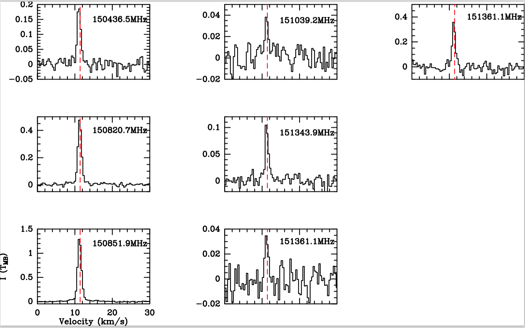
Figure 9: c-C₃H₂ spectra observed towards OMC–2 FIR 4 at 2 mm with the IRAM 30-m telescope. Dashed red lines indicate a $V_{LSR}=11.4$ km s^-1. The frequency the observed transition is indicated on each plot.

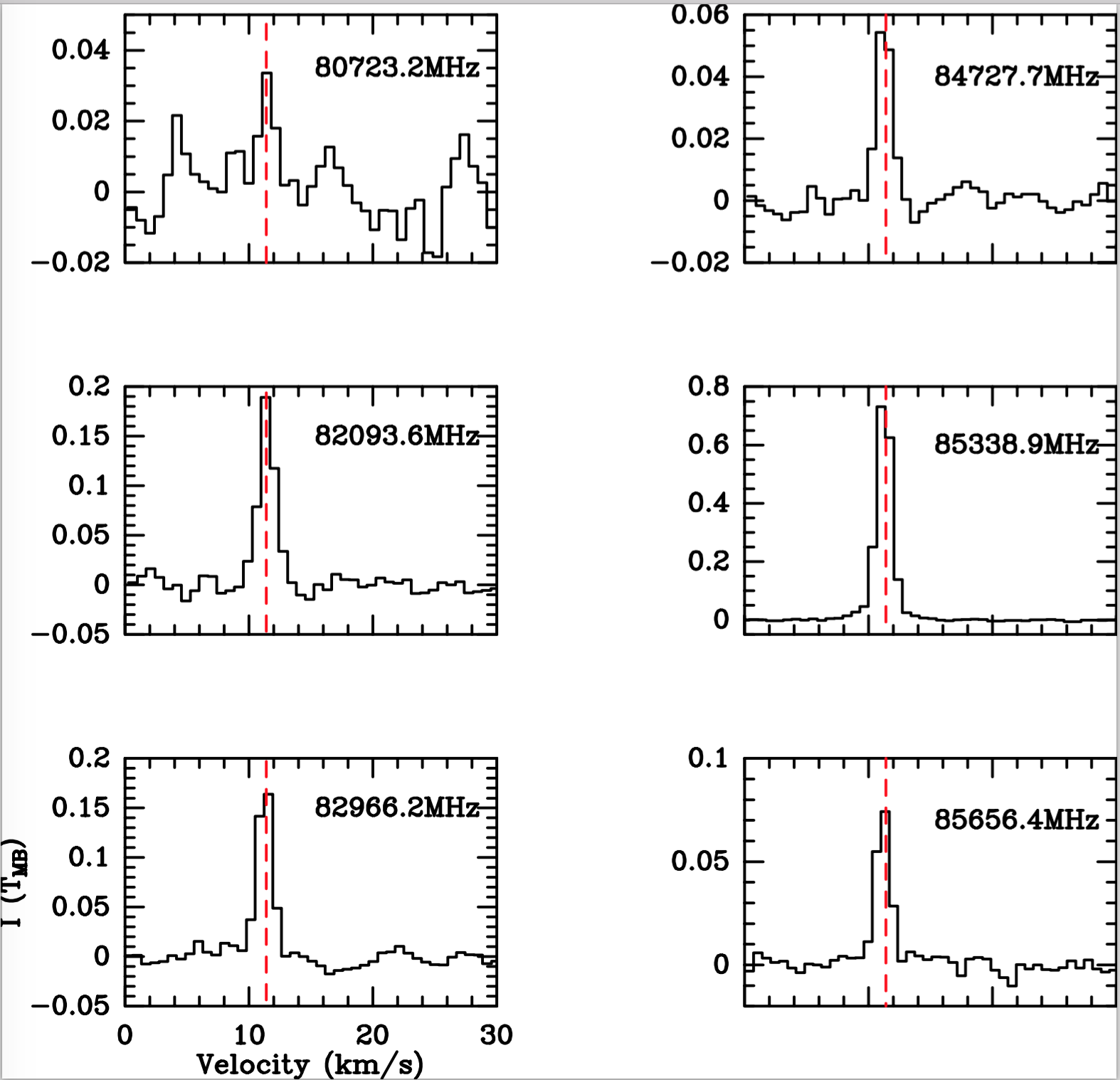
Figure 10: c-C₃H₂ spectra observed towards OMC–2 FIR 4 at 3 mm with the IRAM 30-m telescope. Dashed red lines indicate a $V_{LSR}=11.4$ km s^-1. The frequency the observed transition is indicated on each plot.

The 30m observations detected 24 c–C₃H₂ lines, 14 from the ortho form and 10 from para. Spectra of the c-C₃H₂ transitions observed with the IRAM 30-m telescope towards OMC–2 FIR 4 are displayed in Figures 8, 9 and 10 in Appendix A. Their properties are reported in Table 2. The lines are peaked around the ambient cloud velocity ($\sim$11 km s^-1) and are narrow (FWHM$\sim$1.0–1.6 km/s), indicating that they are emitted by the dense envelope surrounding FIR4 (see Sec. 4).

Table 2: c–C₃H₂ lines detected with the IRAM 30m telescope.

Freq.	Eup	A	Intensitya	FWHMc
(GHz)	(K)	(10-5 s-1)	K km/s	km/s
80.7232	28.8	1.5	0.058 $\pm$ 0.006	1.6
82.0936b	6.4	2.1	0.310 $\pm$ 0.030	1.6
82.9662b	16.0	1.1	0.290 $\pm$ 0.030	1.5
84.7277	16.1	1.2	0.100 $\pm$ 0.010	1.5
85.3389b	6.4	2.6	1.200 $\pm$ 0.120	1.4
85.6564	29.1	1.7	0.120 $\pm$ 0.010	1.4
150.4365	9.7	5.9	0.240 $\pm$ 0.050	1.2
150.8207	19.3	18.0	0.590 $\pm$ 0.120	1.2
150.8519	19.3	18 0	1.700 $\pm$ 0.340	1.2
151.0392	54.7	6.9	0.043 $\pm$ 0.009	1.1
151.3439	35.4	4.4	0.110 $\pm$ 0.020	1.1
151.3611	35.4	4.4	0.042 $\pm$ 0.008	1.1
155.5183	16.1	12.3	0.400 $\pm$ 0.080	1.1
204.7889	28.8	13.7	0.130 $\pm$ 0.030	1.1
216.2788	19.5	28.1	0.740 $\pm$ 0.150	1.0
217.8221	38.6	59.3	1.360 $\pm$ 0.270	1.2
217.9400	35.4	44.3	0.700 $\pm$ 0.140	1.1
218.1604	35.4	44.4	0.270 $\pm$ 0.050	1.1
227.1691	29.1	34.2	0.630 $\pm$ 0.120	1.0
244.2221	18.2	6.5	0.230 $\pm$ 0.050	1.2
249.0544	41.0	45.7	0.280 $\pm$ 0.060	1.1
251.3143	50.7	93.5	0.870 $\pm$ 0.170	1.2
254.9876	41.1	51.7	0.120 $\pm$ 0.020	1.0
260.4797	44.7	17.7	0.080 $\pm$ 0.020	1.1

We used the spectroscopic data parameters from Bogey et al. (1986), Vrtilek et al. (1987), Lovas et al. (1992) and Spezzano et al. (2012), that are available from the Cologne Database for Molecular Spectroscopy molecular line catalog (CDMS, Müller et al., 2005). The Einstein coefficients assume an ortho-to-para ratio of 3:1.
NOTES: ^aThe error in the intensity is the quadratic sum of the statistical and calibration errors. ^bThe emission from this line was imaged by NOEMA. ^cThe FWHM result from gaussian fit.

3.3 Missing flux

To estimate the fraction of the total flux that is filtered out in our interferometric data, we compared the NOEMA to the IRAM 30m lines. More specifically, the NOEMA spectra were convolved with a Gaussian beam similar to that of the 30m beam (i.e. $\sim$30$\arcsec$ at 82–83 GHz). The convolution was performed at the central position of the IRAM 30m observations (see Sec. 2). Finally, the IRAM-30m spectra were smoothed to the same spectral resolution ($\sim$7.2 km s^-1) as that of the NOEMA WideX spectra. The comparison of the integrated line fluxes shows that 57$\%$ of the c-C₃H₂ 2_0,2–1_1,1 emission, 60$\%$ of that of 3_1,2–3_0,3 and 80$\%$ of that of 2_1,2–1_0,1 lines is resolved out. Therefore, the c–C₃H₂ emission detected by NOEMA very likely probes the densest part of the envelope surrounding FIR4 and not the ambient cloud.

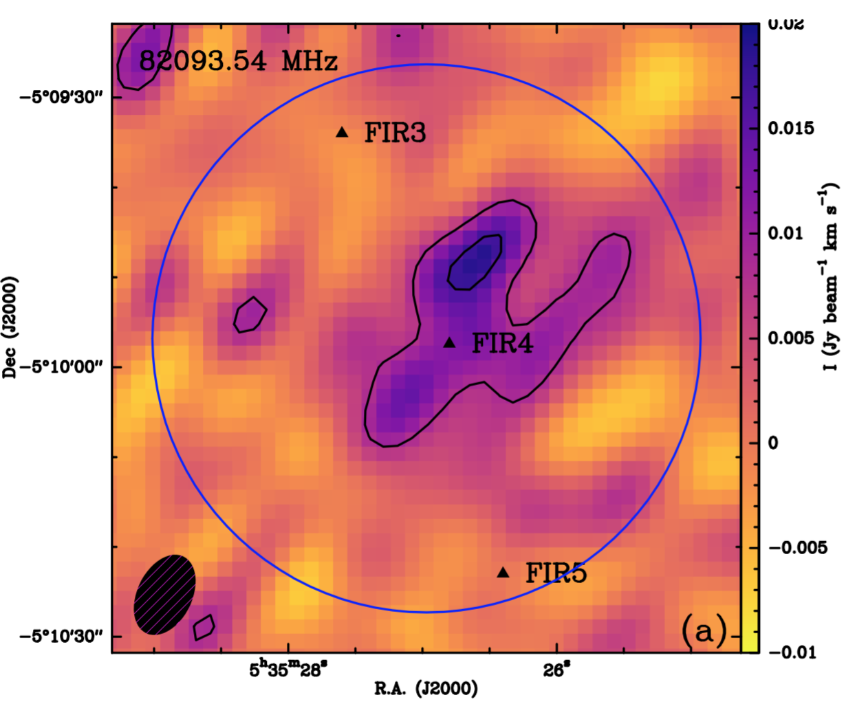
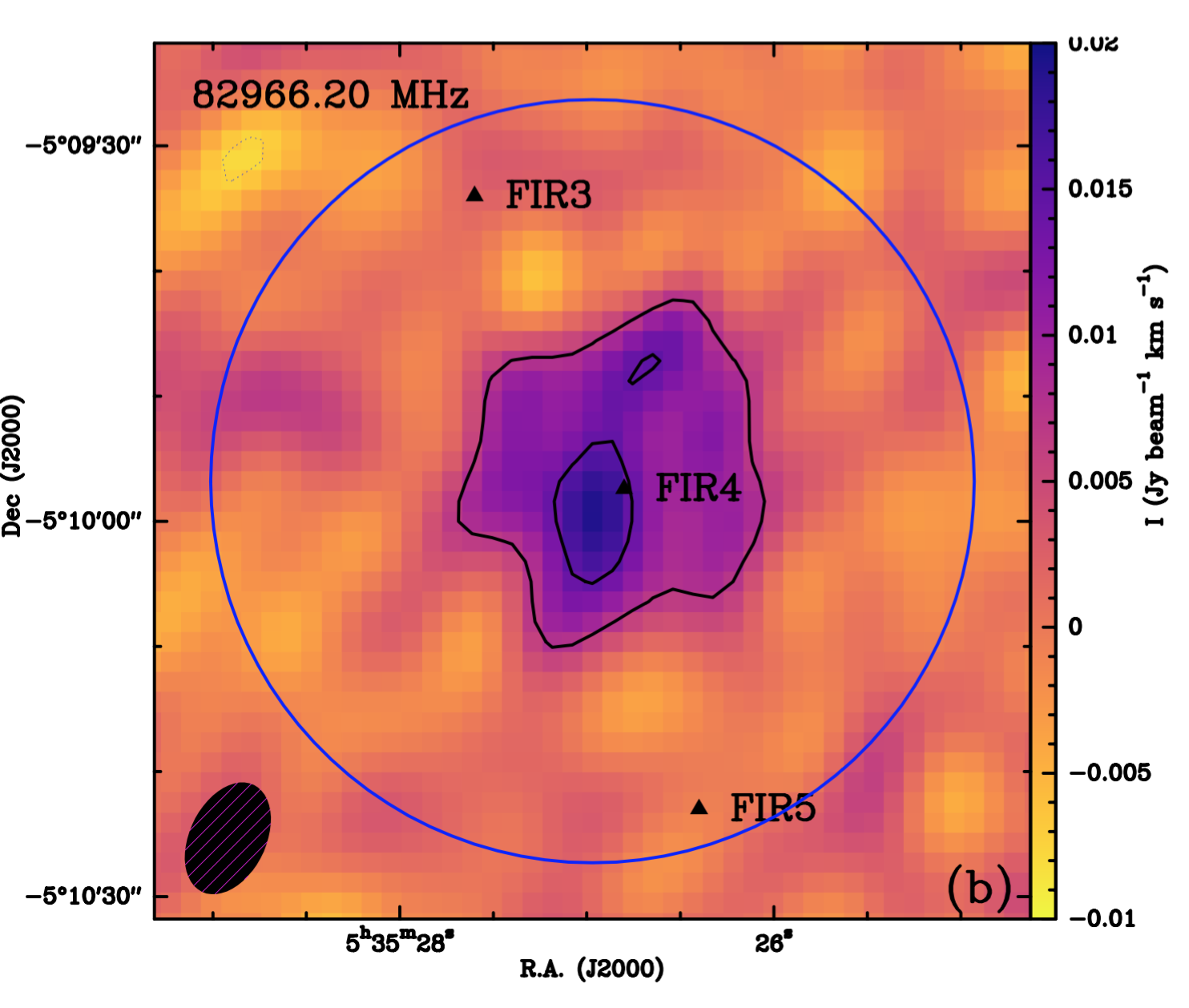
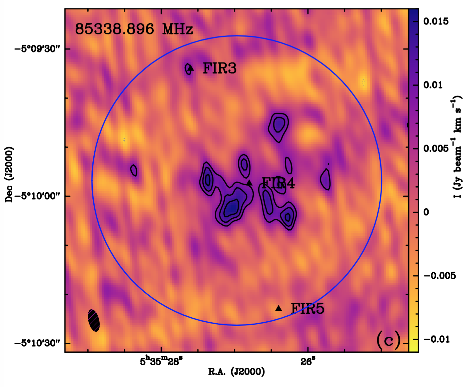
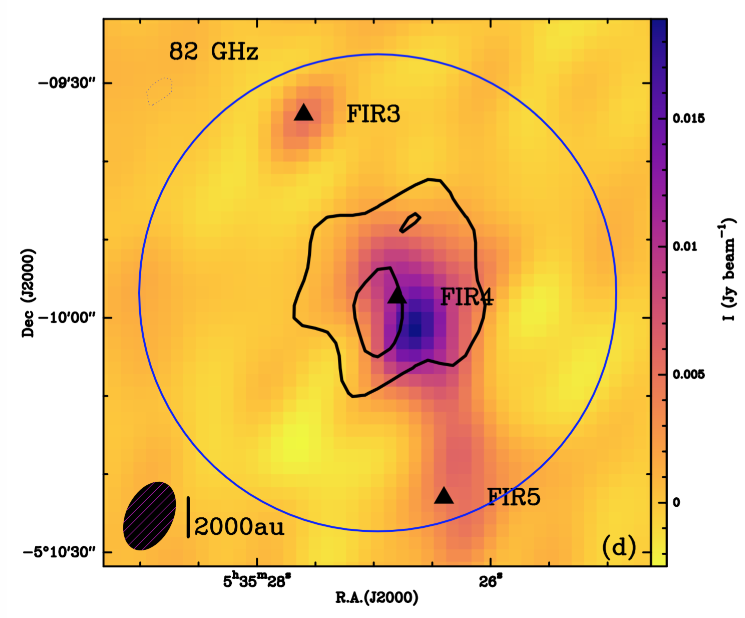
Figure 1: Panel a: c–C₃H₂ (2_0,2–1_1,1) integrated intensity emission map (between 0 and 22 km s^-1). The contour levels are at 3$\sigma$ and 6$\sigma$ (where 1$\sigma$=2.76$\times$10^-3 Jy beam^-1 km s^-1). Panel b: c–C₃H₂ (3_1,2–3_0,3) integrated intensity emission map (between 0 and 22 km s^-1). The contour levels are at 3$\sigma$ and 6$\sigma$ (where 1$\sigma$=2.4$\times$10^-3 Jy beam^-1 km s^-1). Panel c: c–C₃H₂ (2_1,2–1_0,1) integrated intensity emission map (between 0 and 22 km s^-1). The contour levels are at 3$\sigma$, 4$\sigma$ and 5$\sigma$ (where 1$\sigma$=2.8$\times$10^-3 Jy beam^-1 km s^-1). Panel d: 82 GHz continuum emission (color) overlaid with the integrated intensity emission map of the c–C₃H₂ (3_1,2–3_0,3) at 82966 MHz (black contours). The contour levels for the continuum and c–C₃H₂ emission maps are the same as in Fontani et al. (2017) and in Panel b . Finally, in Panels a, b, c and d, the black triangles indicate the positions of the FIR3, FIR4 and FIR5 regions (see Chini et al., 1997); and the blue circle shows the NOEMA field of view.

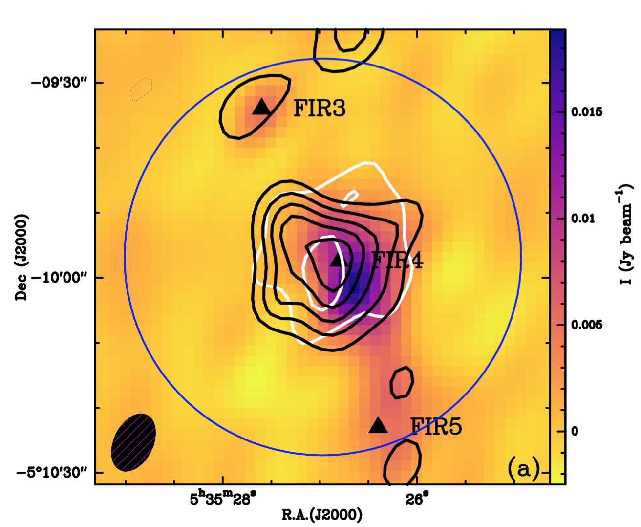
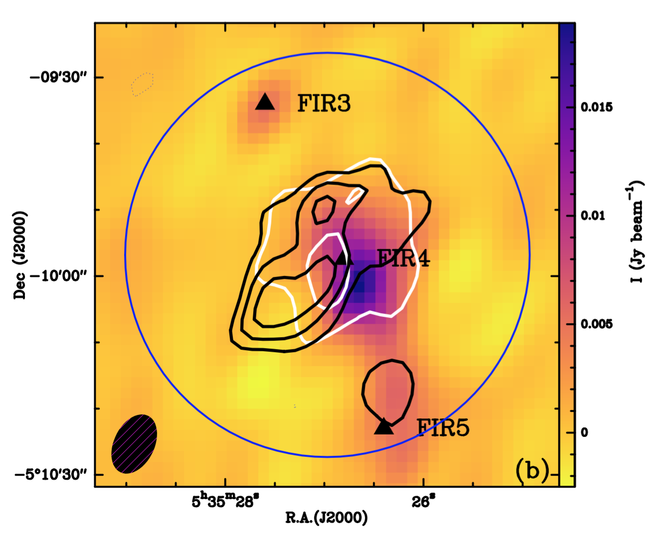
Figure 2: Panel a: 82 GHz continuum emission (color) overlaid with the integrated intensity emission map of the c–C₃H₂ (3_1,2–3_0,3) at 82.97 GHz (white contours) and that of the HC₃N (9–8) at 81.88 GHz (black contours; from Fontani et al., 2017). Panel b 82 GHz continuum emission (color) overlaid with the integrated intensity emission map of the c–C₃H₂ (3_1,2–3_0,3) at 82.97 GHz (white contours) and that of the HC₅N (31–30) at 82.54 GHz (black contours; from Fontani et al., 2017). Finally, in Panels a and b, the contour levels for the continuum, HC₃N and HC₅N maps are the same as in Fontani et al. (2017). Contour levels for the c–C₃H₂ emission map are given in Figure 1. The blue circle shows the NOEMA field of view.

4 Temperature and c-C₃H₂ column density

4.1 Average properties of the FIR4 envelope

We first derive the average properties of the FIR4 envelope using the IRAM 30m data. To this end, we first carried out a simple LTE analysis, and then a non-LTE one.

4.1.1 LTE analysis

The rotational diagram, obtained assuming an ortho-to-para ratio equal to 3 and a beam filling factor equal to 1, is shown in Fig. 3. No systematic difference is seen between ortho and para lines, which implies that our assumption on the ortho-to-para ratio is basically correct.

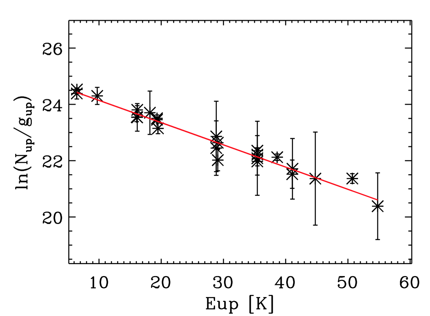
Figure 3: Rotational diagram derived from the c-C₃H₂ lines detected with the IRAM 30m telescope (Table 2). The ortho-to-para ratio is taken equal to 3. The error bars correspond to the 1$\sigma$ Gaussian fit uncertainties.

The derived rotational temperature is (12.6$\pm$0.5) K and the c-C₃H₂ column density is (7$\pm$1)$\times 10^{12}$ cm^-2. Assuming that the emission arises from a 20^′′ region (see below), would not change much these results: it would give (10.7$\pm$0.5) K and (1.5$\pm$0.2)$\times 10^{13}$ cm^-2, respectively, and a slightly worse (but not significantly better) $\chi^{2}_{red}$ (0.08 instead of 0.05).

4.1.2 non-LTE analysis

Given the large number of c-C₃H₂ lines, we carried out a non-LTE analysis assuming the Large Velocity Gradient (LVG) approximation. To this end, we used the LVG code described in Ceccarelli et al. (2002) and used the collisional coefficients with He, after scaling for the different mass of H₂, computed by Chandra & Kegel (2000) and retrieved from the BASECOL database. We assumed a c-C₃H₂ ortho-to-para ratio equal to 3, as suggested by the LTE analysis.

We ran a large grid of models with H₂ density between $3\times 10^{4}$ and $5\times 10^{6}$ cm^-3, temperature between 10 and 50 K and c-C₃H₂ column density between $3\times 10^{12}$ and $2\times 10^{13}$ cm^-2. We adopted a FWHM of 1.3 km s^-1 and let the filling factor be a free parameter. We then compared the LVG predictions with the observations and used the standard minimum reduced $\chi^{2}$ criterium to constrain the four parameters: H₂ density, temperature, column density and size. In practice, for each column density we found the minimum $\chi^{2}$ in the density-temperature-size parameter space. The solution then is the one with the c-C₃H₂ column density giving the smallest $\chi^{2}$.

The best fit is obtained for an extended source (i.e. $\geq 30^{\prime\prime}$), c-C₃H₂ column density equal to (7$\pm$1)$\times 10^{12}$ cm^-2 (in excellent agreement with the LTE estimate), temperature equal to 40 K and density equal to $3\times 10^{5}$ cm^-3. At 2$\sigma$ level, the solution becomes degenerate in the density-temperature parameter space. A family of solutions are possible, with the two extremes at 15 K and $5\times 10^{6}$ cm^-3 on one side, and 50 K and $2\times 10^{5}$ cm^-3 on the other side. Please note that, indeed, the coldest and densest solution provides a temperature close to the rotational temperature (13 K). This means that the apparent LTE distribution of the transition levels derived by the IRAM 30m line intensities is also obtained with non-LTE conditions and the densities and temperatures mentioned above, included the best fit solution. Finally, in all cases, the lines are optically thin. In the following, we will use the best fit solution and we will associate the errors as follows: (40$\pm$10) K and ($3\pm 1$) $\times 10^{5}$ cm^-3.

Assuming a H₂ column density measured from the continuum by Fontani et al. (2017), $\sim 10^{24}$ cm^-2, we obtain an average c-C₃H₂ abundance of (7$\pm$1)$\times 10^{-12}$, assuming that c-C₃H₂ is present across the entire OMC–2 FIR 4 region (Section 5).

4.2 The structure of the FIR4 envelope

The maps obtained with the NOEMA interferometer allow us to estimate the gas temperature and the c-C₃H₂ abundance across the region probed by the NOEMA observations.

To measure the excitation temperature, we use the two c-C₃H₂ lines at 82 GHz, which have the same spatial resolution and, most importantly, the same amount of filtered out extended emission. To this end, we assumed that (1) the c–C₃H₂ ortho-to-para ratio is equal to 3, (2) the lines are optically thin, and (3) the levels are LTE populated. With this assumptions, we derived the excitation temperature map shown in Figure 4, along with the associated uncertainty. The excitation temperature is comprised between 8$\pm$3 and 16$\pm$7 K (i.e. minimum and maximum values, see Fig. 4). When considering the uncertainty on the values, there are no signs of excitation temperature gradients across the region we are probing (about 3-4 beams). On the contrary, the excitation temperature seems to be rather constant and not much different from that probed by the 30m data analysis ($\sim$12 K) (see previous section).

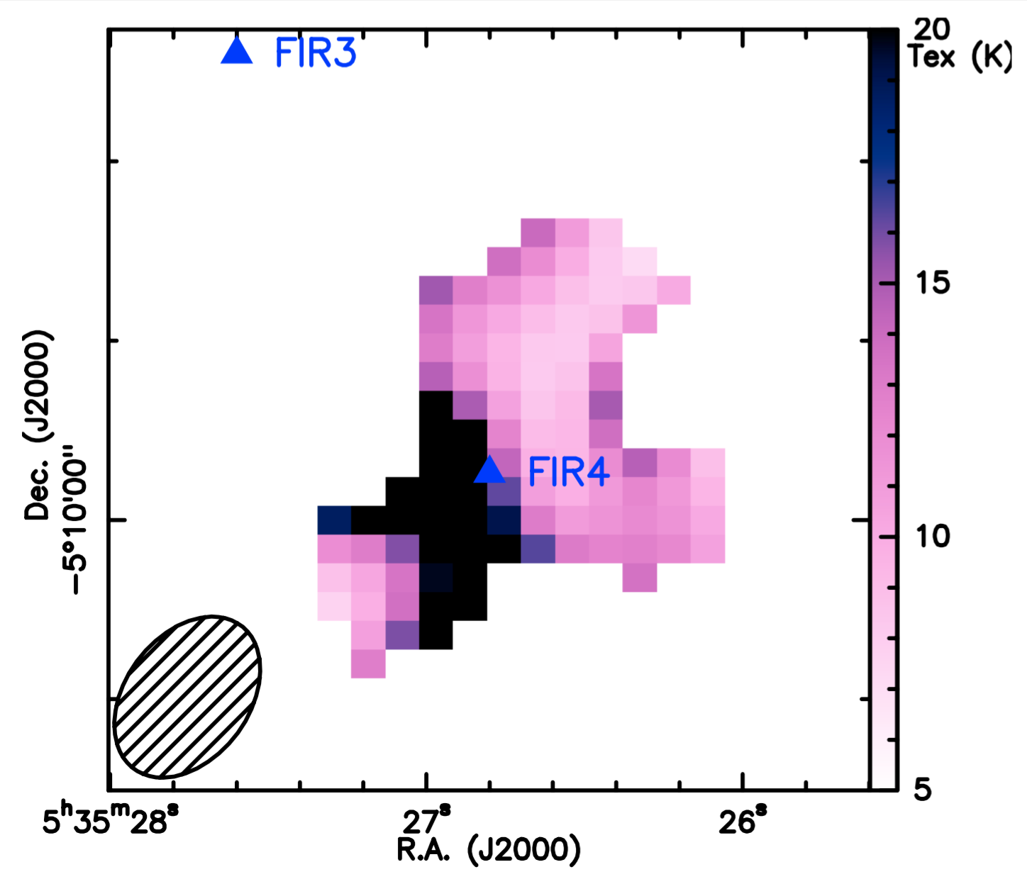
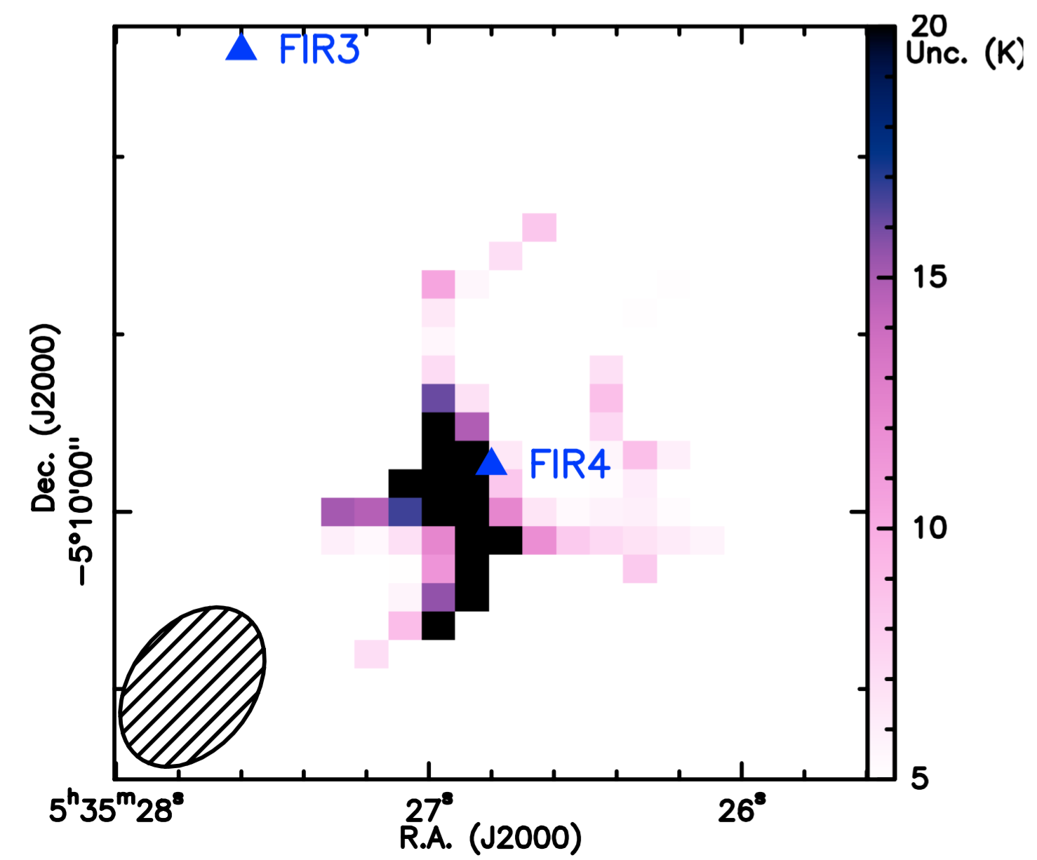
Figure 4: c–C₃H₂ excitation temperature map towards OMC2–FIR4 (top panel) along with the uncertainty map (bottom panel).

5 Chemical modeling

In the previous Section, we showed that the gas emitting the c–C₃H₂ lines has a temperature of $\sim 40$ K and H₂ density $\sim 3\times 10^{5}$ cm^-3. The c–C₃H₂ column density is $\sim 7\times 10^{12}$ cm^-2. In this section, we use a Photo-Dissociation Region (PDR) model to understand the structure of the gas probed by the c–C₃H₂ lines, notably where they come from, and what constraints they provide.

To this end, we used the Meudon PDR code (version 1.5.2, see Le Petit et al., 2006; Bron et al., 2016). The code computes the steady-state thermal and chemical structure of a cloud irradiated by a FUV radiation field $G_{o}$ and permeated by CR that ionise the gas at a rate $\zeta_{CR}$. Relevant to the chemistry, the code computes the gas-phase abundances of the most abundant species, including c–C₃H₂. In our simulations, we adopted the density derived by the c–C₃H₂ non-LTE analysis ($n_{H}=6\times 10^{5}$ cm^-3) and the elemental abundances listed in Table 3. Note that we limited the PDR simulations to a H-nuclei column density N_H of $\sim 4\times 10^{22}$ cm^-2 (corresponding to A_v=20 mag; see Figs. 5 and 6). However, to compare the final predicted c–C₃H₂ column density, N_Tot, with the observed one ($7\times 10^{12}$ cm^-2), we have to consider the whole cloud, which has a total H-nuclei column density N${}_{H}^{FIR4}$ of $2\times 10^{24}$ cm^-2 (Fontani et al., 2017). Therefore, we multiplied the c–C₃H₂ abundance predicted by the model in the cloud interior X_interior (computed by the code at N${}_{H}=3\times 10^{22}$ cm^-2) by N${}_{H}^{FIR4}$, and added it to the c–C₃H₂ column density in the PDR region N_PDR (computed by the code for N${}_{H}\leq 1\times 10^{22}$ cm^-2), as follows:

$${\rm N}_{Tot}={\rm X}_{interior}\times{\rm N}_{H}^{FIR4}+2\times{\rm N}_{PDR}$$ (1)

Element	Abundance	Element	Abundance
O	$3.2\times 10^{-4}$	C	$1.3\times 10^{-4}$
N	$7.5\times 10^{-5}$	S	$1.9\times 10^{-5}$
Si	$8.2\times 10^{-7}$	Fe	$1.5\times 10^{-8}$

Table 3: Assumed elementary abundances, with respect to H nulei, in the PDR modeling.

To initialize our grid of models, we used as input parameter a temperature of 50 K, and assume an edge-on region that is irradiated from one side only. Then, we run several models with values of $G_{0}$ ($G_{0}=$ is the FUV radiation field in Habing units) ranging from 1 to 1700, and $\zeta_{CR}$ from $1\times 10^{-16}$ s^-1 to $4\times 10^{-14}$ s^-1. These extreme values are quoted in the literature for the OMC–2 region (see Introduction and Discussion). Note that, even though we did not run a full grid of models, we fine-tuned the parameter ranges close to the best fit solution.

Model	$\zeta_{CR}$	$G_{0}$	NPDR	Xinterior	NTot	Tgas
	($10^{-16}$ s-1)		($10^{12}$ cm-2)		($10^{12}$ cm-2)	(K)
1	1	1	0.01	$9.8\times 10^{-16}$	0.02	9
2	1	10	0.05	$1.5\times 10^{-15}$	0.1	9
3	1	1700	0.75	$2.5\times 10^{-14}$	1.5	17
4	20	100	0.11	$5.3\times 10^{-13}$	1.3	14
5	20	1700	0.77	$7.1\times 10^{-13}$	2.9	20
6	100	10	0.12	$5.7\times 10^{-13}$	1.4	23
7	100	100	0.18	$1.6\times 10^{-12}$	3.7	25
8	100	1700	0.79	$1.5\times 10^{-12}$	4.6	29
9	400	1	0.06	$7.4\times 10^{-13}$	1.6	41
10	400	10	0.19	$1.1\times 10^{-12}$	2.5	42
11	400	100	0.26	$2.2\times 10^{-12}$	5.0	43
12	400	1700	0.86	$2.4\times 10^{-12}$	6.5	45

Table 4: List of the $\zeta_{CR}$ and $G_{0}$ values adopted for the different PDR models and the results of the simulations: the c-C₃H₂ column density in the PDR region, N_PDR; the c-C₃H₂ abundance (with respect to H nuclei) in the inetrior (see text), X_interior; the total c-C₃H₂ column density, N_Tot, which takes into account the whole cloud (see text); the gas temperature (in the interior).

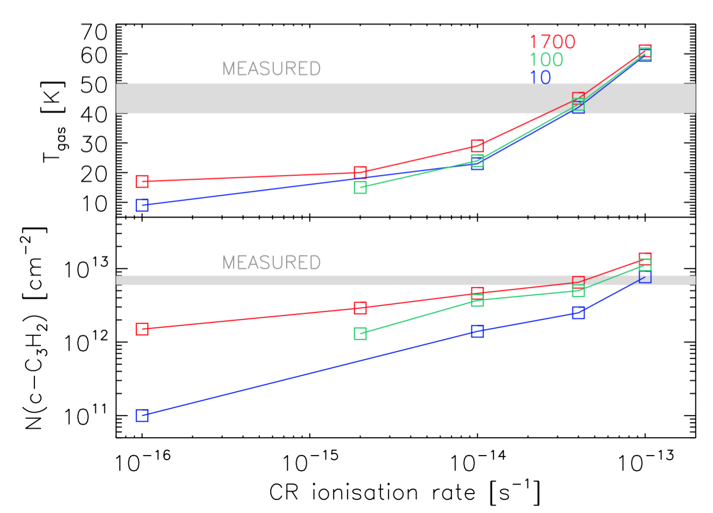
Figure 5: Results of the PDR modeling: predicted c-C₃H₂ column density (lower panel) and gas temperature (upper panel) as a function of the CR ionisation rate $\zeta_{CR}$, for a FUV field $G_{0}$ equal to 1700 (red), 100 (green) and 10 (blue), respectively. Symbols show the actual runs.

The run models and the associated results are listed in Table 4 and shown in Figure 5. Both the predicted c-C₃H₂ column density and gas temperature are strong functions of $\zeta_{CR}$: the larger $\zeta_{CR}$ the larger the column density and the temperature. On the contrary, the value of $G_{0}$ has a small influence on the predicted values, in particular for the temperature.

The comparison of the PDR modeling results (Table 4 and Figure 5) with the measured c-C₃H₂ column density and gas temperature very clearly indicates that the gas is permeated by a large flux of CR and is irradiated by an intense FUV field. Specifically, model 12 ($\zeta_{CR}=4\times 10^{-14}$ s^-1 and $G_{0}=1700$) reproduces fairly well the measured c-C₃H₂ column density ($\sim 7\times 10^{12}$ cm^-2) and gas temperature ($\sim 40$ K).

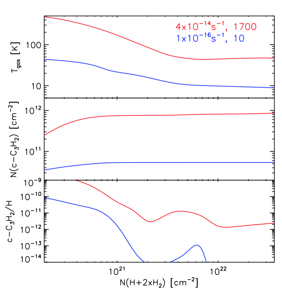
Figure 6: Thermal and chemical structure of two models: predicted gas temperature (upper panel), c-C₃H₂ column density in the PDR (middle panel) and abundance (bottom panel) as a function of the H nuclei column density. Two models are reported: model 12 ($\zeta_{CR}=4\times 10^{-14}$ s^-1 and $G_{0}=1700$; red), and model 2 ($\zeta_{CR}=1\times 10^{-16}$ s^-1 and $G_{0}=10$; blue).

Figure 6 shows the gas temperature, the c-C₃H₂ abundance and column density as a function of N(H+2$\times$H₂) for the model 12, which best reproduces the observations, and model 2, for comparison.

In general, the c-C₃H₂ abundance has a first peak in the PDR region, in a tiny layer at N(H+2$\times$H₂) $\leq\times 10^{21}$ cm^-2. This first peak depends on the FUV radiation field and increases with increasing $G_{0}$. In the interior of the cloud, at N(H+2$\times$H₂) $\geq\times 10^{22}$ cm^-2, namely in the region that contributes most to the total c-C₃H₂ column density, the c-C₃H₂ abundance is governed by the CR ionisation rate and increases with $\zeta_{CR}$. As expected, the gas temperature at the PDR border is governed by the FUV field, whereas it is governed by CR ionisation rate in the interior.

6 Discussion

6.1 OMC–2 FIR 4: a highly irradiated region

In the previous section, we showed that in order to reproduce the temperature of the gas probed by the c-C₃H₂ lines and its abundance the gas has to be irradiated by a strong flux of CR-like particles. Amazingly, the best agreement between observations and model predictions is given by a CR ionisation rate, $\zeta_{CR}=4\times 10^{-14}$ s^-1, that is the same as the one derived by the following observations: (1) the HCO⁺ and N₂H⁺ high J lines observed by Herschel HIFI CHESS project (Ceccarelli et al., 2014), and (2) the HC₃N and HC₅N lines observed by NOEMA SOLIS project (Fontani et al., 2017). In addition, the c-C₃H₂ emitting region roughly coincides with the largest $\zeta_{CR}$ region which is probed by the HC₅N emission area. We emphasise that, in addition to being different data sets and different species, the three estimates of $\zeta_{CR}$ have been obtained also with three different astrochemical codes: ASTROCHEM, Nahoon (Wakelam et al., 2012) and Meudon PDR (version 1.5.2, Le Petit et al., 2006; Bron et al., 2016) codes.

The emerging picture is shown in the cartoon of Figure 7. Previous Herschel HIFI CHESS observations showed that between OMC–2 and us there is a tenuous ($100$ cm^-3) cloud extending about 6 pc along the line of sight, and illuminated by a FUV field about 1000 times brighter than the interstellar standard radiation field (López-Sepulcre et al., 2013a). OMC–2 itself hosts three FIR sources (FIR 3, 4 and 5), which are likely very different in nature and evolutionary status, even though not much is known especially about FIR3 and FIR5, except that a large-scale ($\sim 30^{\prime\prime}$) outflow emanates from FIR3 (Takahashi et al., 2008; Shimajiri et al., 2008, 2015). FIR4 is actually a dense clump ($\sim 10^{5}-10^{6}$ cm^-3: Crimier et al., 2009; Ceccarelli et al., 2014) with an embedded cluster of young sources, whose number is still unclear (Shimajiri et al., 2008; López-Sepulcre et al., 2013b; Kainulainen et al., 2017). What is clear now is that FIR4 is permeated by a flux of CR-like ionising particles about 1000 times larger than the CR flux of the Galaxy. The source(s) of these particles is(are) likely situated in the East part of FIR4 (Fontani et al., 2017), but still remains unidentified. Incidentally, it is important to note that the high CR ionization rate could result in a temperature gradient in the vicinity of the CR emitting source(s). Nonetheless, the c-C₃H₂ excitation temperature mainly covers the west region (see Figure 4), where the irradiation is likely lower, based on the HC₅N/HC₃N abundance ratio by Fontani et al. (2017). The new IRAM 30m and SOLIS observations presented in this work confirm this geometry and indicate that abundant hydrocarbons (c-C₃H₂) are present not only at the skin of the FIR4 clump but also in the interior, because of the strong CR-like irradiation.

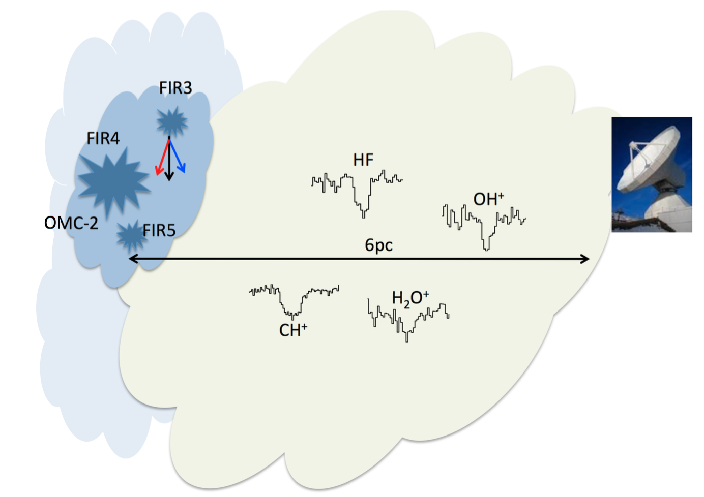
Figure 7: Cartoon of OMC–2. A tenuous cloud between OMC–2 and the Sun is probed by the absorption of HF, OH⁺, CH⁺ and H₂O⁺ observed by the Herschel HIFI instrument (López-Sepulcre et al., 2013a). The OMC–2 complex is associated with three FIR sources: FIR3, FIR4 and FIR5, respectively. An outflow is emitted by FIR3 which, based on the present observations, is unlikely impacting the FIR4 envelope.

6.2 No evidence of the FIR3 outflow impact on FIR4

It has been suggested that the chemical composition of OMC–2 FIR4 is affected by the interaction of the northeast–southwest outflow driven by the nearby source FIR3 (see Shimajiri et al., 2008, 2015), which is located at about 23$\arcsec$ northeast from FIR4 (i.e. $\sim$9660 AU at a distance of 420 pc, Menten et al., 2007; Hirota et al., 2007). Specifically, Shimajiri et al. (2008, 2015) have suggested that gas associated with OMC–2 FIR4 might be impacted by this NE-SW outflow. If this is the case, the gas associated with the envelope of the OMC–2 FIR4 region should show some physically induced effect. In this instance, the c-C₃H₂ molecular emission map would likely present a temperature gradient within the region. This is not the case in our observations (see Figure 4) which, contrary to Shimajiri et al. (2015), probe the envelope of OMC–2 FIR4 and not the ambient gas thanks to the interferometer spatial filtering. These findings lead one to ask whether the apparent spatial coincidence of the southern outflow lobe driven by FIR3 and the northern edge of FIR4 is simply a projection effect. More sensitive, higher angular resolution observations may help us confirm our current conclusion.

7 Conclusions

We have imaged, for the first time, the distribution of cyclopropenylidene, c–C₃H₂, towards OMC–2 FIR 4 with an angular resolution of 9.5″$\times$6.1″at 82 GHz and 4.7″$\times$2.2″at 85 GHz, using NOEMA. The observations were performed as part of the SOLIS program. In addition, we have performed a study of the physical properties of this source through the use of IRAM-30m observations.

Our main results and conclusions are the following:

1. From a non-LTE analysis of the IRAM-30m data, we find that c–C₃H₂ gas emits at the average temperature of about 40 K with a $\chi$(c–C₃H₂) abundance of ($7\pm 1$)$\times 10^{-12}$.

2. Our NOEMA observations show that there is no sign of excitation temperature gradients within the observed region (which corresponds to $\sim$3-4 beams), with a T_ex(c–C₃H₂) in the range 8$\pm$3 – 16$\pm$7 K. Our findings suggest that the OMC–2 FIR 4 envelope is not in direct physical interaction with the outflow originating from OMC–2 FIR 3.

3. In addition, the c–C₃H₂ gas probed by NOEMA arises from the same region as that of HC₅N which is a probe of high CR-particles ionization (Fontani et al., 2017).

4. Finally, a notable result, derived from chemical modelling with the Meudon PDR code is that OMC–2 FIR 4 appears to be a strongly irradiated region: FUV field dominates the outer shells (with a radiation field scaling factor $G_{0}$ of about 1700) while the interior of the envelope is governed by CR ionization (with a CR ionization rate $\zeta_{CR}$ = $4\times 10^{-14}$ s^-1, namely more than a thousand times the canonical value).

These results are consistent with previous studies claiming that OMC–2 FIR 4 bathes in an intense radiation field of energetic particles ($\geq 10$ MeV).

8 Acknowledgements

We warmly thank Franck Le Petit for his assistance in the use of the PDR code. CF acknowledge the financial support for this work provided by the French space agency CNES along with the support from the Italian Ministry of Education, Universities and Research, project SIR (RBSI14ZRHR). We acknowledge the funding from the European Research Council (ERC), projects PALs (contract 320620) and DOC (contract 741002). This work was supported by the French program “Physique et Chimie du Milieu Interstellaire” (PCMI) funded by the Conseil National de la Recherche Scientifique (CNRS) and Centre National d’ Etudes Spatiales (CNES) and by the Italian Ministero dell’Istruzione, Universitá e Ricerca through the grant Progetti Premiali 2012 - iALMA (CUP C52I13000140001).

Appendix A c-C₃H₂ towards OMC–2 FIR 4 as observed with IRAM-30m telescope

Figures 8 to 10 display the spectra of the c-C₃H₂ transitions observed with the IRAM 30-m telescope towards OMC–2 FIR 4 at 1, 2 and 3 mm, respectively.

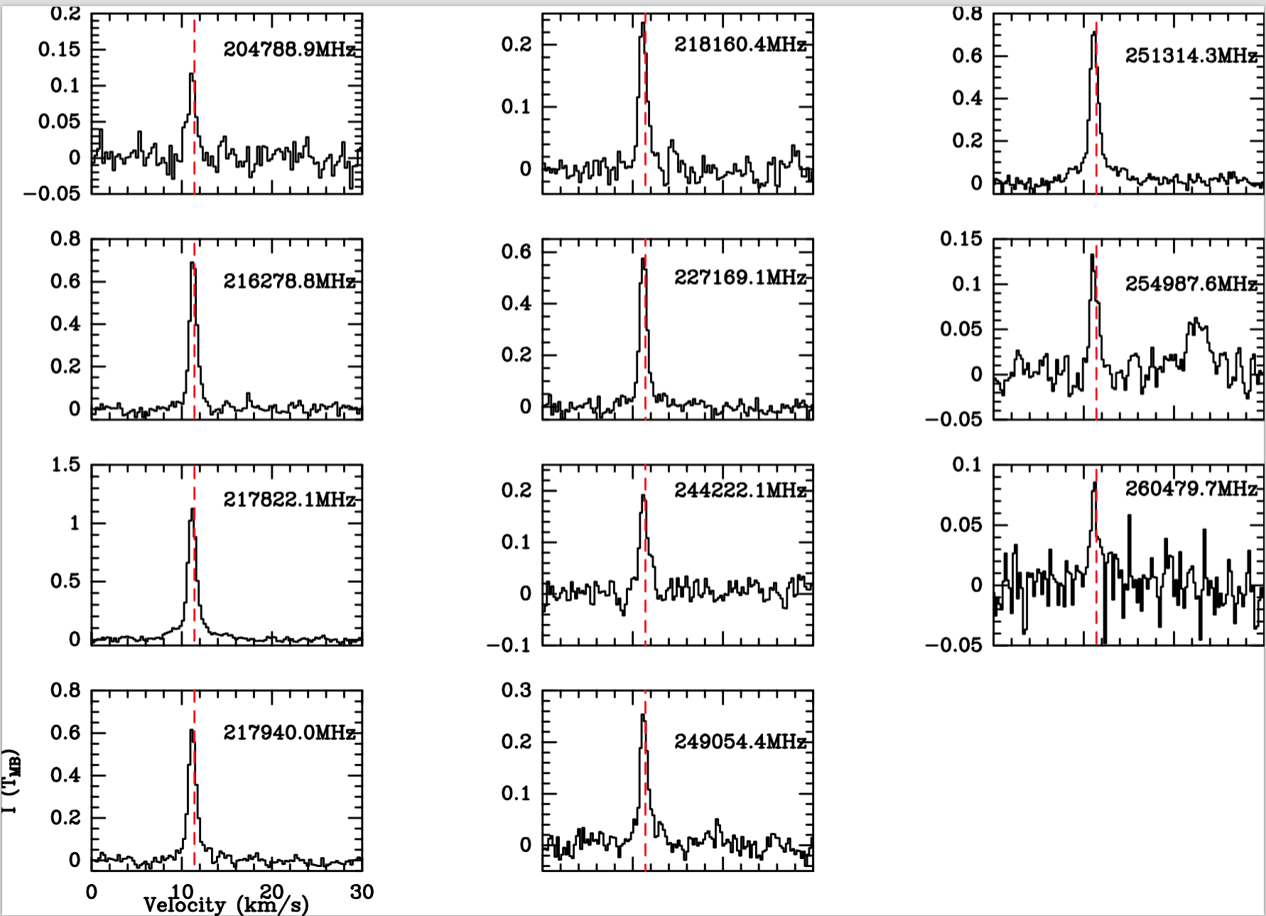
Figure 8: c-C₃H₂ spectra observed towards OMC–2 FIR 4 at 1 mm with the IRAM 30-m telescope. Dashed red lines indicate a $V_{LSR}=11.4$ km s^-1. The frequency the observed transition is indicated on each plot.

References

- Adams (2010) Adams, F. C. 2010, ARA&A, 48, 47
- Bogey et al. (1986) Bogey, M., Demuynck, C., & Destombes, J. L. 1986, Chemical Physics Letters, 125, 383
- Bron et al. (2016) Bron, E., Le Petit, F., & Le Bourlot, J. 2016, A&A, 588, A27
- Caselli & Ceccarelli (2012) Caselli, P., & Ceccarelli, C. 2012, A&A Rev., 20, 56
- Ceccarelli et al. (2014) Ceccarelli, C., Dominik, C., López-Sepulcre, A., et al. 2014, ApJ, 790, L1
- Ceccarelli et al. (2002) Ceccarelli, C., Baluteau, J.-P., Walmsley, M., et al. 2002, A&A, 383, 603
- Ceccarelli et al. (2017) Ceccarelli, C., Caselli, P., Fontani, F., et al. 2017, ApJ, 850, 176
- Chandra & Kegel (2000) Chandra, S., & Kegel, W. H. 2000, A&AS, 142, 113
- Chini et al. (1997) Chini, R., Reipurth, B., Ward-Thompson, D., et al. 1997, ApJ, 474, L135
- Crimier et al. (2009) Crimier, N., Ceccarelli, C., Lefloch, B., & Faure, A. 2009, A&A, 506, 1229
- Dubernet et al. (2013) Dubernet, M.-L., Alexander, M. H., Ba, Y. A., et al. 2013, A&A, 553, A50
- Fontani et al. (2017) Fontani, F., Ceccarelli, C., Favre, C., et al. 2017, A&A, 605, A57
- Gounelle et al. (2013) Gounelle, M., Chaussidon, M., & Rollion-Bard, C. 2013, ApJ, 763, L33
- Hirota et al. (2007) Hirota, T., Bushimata, T., Choi, Y. K., et al. 2007, PASJ, 59, 897
- Högbom (1974) Högbom, J. A. 1974, A&AS, 15, 417
- Kainulainen et al. (2017) Kainulainen, J., Stutz, A. M., Stanke, T., et al. 2017, A&A, 600, A141
- Le Petit et al. (2006) Le Petit, F., Nehmé, C., Le Bourlot, J., & Roueff, E. 2006, ApJS, 164, 506
- López-Sepulcre et al. (2013a) López-Sepulcre, A., Kama, M., Ceccarelli, C., et al. 2013a, A&A, 549, A114
- López-Sepulcre et al. (2013b) López-Sepulcre, A., Taquet, V., Sánchez-Monge, Á., et al. 2013b, A&A, 556, A62
- López-Sepulcre et al. (2015) López-Sepulcre, A., Jaber, A. A., Mendoza, E., et al. 2015, MNRAS, 449, 2438
- Lovas et al. (1992) Lovas, F. J., Suenram, R. D., Ogata, T., & Yamamoto, S. 1992, ApJ, 399, 325
- Menten et al. (2007) Menten, K. M., Reid, M. J., Forbrich, J., & Brunthaler, A. 2007, A&A, 474, 515
- Müller et al. (2005) Müller, H. S. P., Schlöder, F., Stutzki, J., & Winnewisser, G. 2005, Journal of Molecular Structure, 742, 215
- Shimajiri et al. (2008) Shimajiri, Y., Takahashi, S., Takakuwa, S., Saito, M., & Kawabe, R. 2008, ApJ, 683, 255
- Shimajiri et al. (2011) Shimajiri, Y., Kawabe, R., Takakuwa, S., et al. 2011, PASJ, 63, 105
- Shimajiri et al. (2015) Shimajiri, Y., Sakai, T., Kitamura, Y., et al. 2015, ApJS, 221, 31
- Spezzano et al. (2012) Spezzano, S., Tamassia, F., Thorwirth, S., et al. 2012, ApJS, 200, 1
- Takahashi et al. (2008) Takahashi, S., Saito, M., Ohashi, N., et al. 2008, ApJ, 688, 344
- Vrtilek et al. (1987) Vrtilek, J. M., Gottlieb, C. A., & Thaddeus, P. 1987, ApJ, 314, 716
- Wakelam et al. (2012) Wakelam, V., Herbst, E., Loison, J.-C., et al. 2012, ApJS, 199, 21