Spectral gap in random bipartite biregular graphs and applications

Abstract.

We prove an analogue of Alon’s spectral gap conjecture for random bipartite, biregular graphs. We use the Ihara-Bass formula to connect the non-backtracking spectrum to that of the adjacency matrix, employing the moment method to show there exists a spectral gap for the non-backtracking matrix. A byproduct of our main theorem is that random rectangular zero-one matrices with fixed row and column sums are full-rank with high probability. Finally, we illustrate applications to community detection, coding theory, and deterministic matrix completion.

1. Introduction

Random regular graphs, where each vertex has the same degree $d$, are among the most well-known examples of expanders: graphs with high connectivity and which exhibit rapid mixing. Expanders are of particular interest in computer science, from sampling and complexity theory to design of error-correcting codes. For an extensive review of their applications, see Hoory, Linial, and Wigderson (2006). What makes random regular graphs particularly interesting expanders is the fact that they exhibit all three existing types of expansion properties: edge, vertex, and spectral.

The study of regular random graphs took off with the work of Bender (1974), Bender and Canfield (1978), Bollobás (1980), and slightly later McKay (1984) and Wormald (1981). Most often, their expanding properties are described in terms of the existence of the spectral gap, which we define below.

Let $A$ be the adjacency matrix of a simple graph, where $A_{ij}=1$ if $i$ and $j$ are connected and zero otherwise. Denote $\sigma(A)=\{\lambda_{1}\geq\lambda_{2}\geq\ldots\}$ as its spectrum. For a random $d$-regular graph, $\lambda_{1}=\max_{i}|\lambda_{i}|=d$, but the second largest eigenvalue $\eta=\max(|\lambda_{2}|,|\lambda_{n}|)$ is asymptoticly almost surely of much smaller order, leading to a spectral gap. Note that we will always use $\eta$ to be the second largest eigenvalue of the adjacency matrix $A$. For a list of important symbols see Appendix A.

Spectral expansion properties of a graph are, strictly speaking, defined with respect to the smallest nonzero eigenvalue of the normalized Laplacian, $\mathcal{L}=I-D^{-1/2}AD^{-1/2}$, where $I$ is the identity and $D$ is the diagonal matrix of vertex degrees. In the case of a $d$-regular graph, $\sigma(\mathcal{L})$ is a scaled and shifted version of $\sigma(A)$. Thus, a spectral gap for $A$ translates directly into one for $\mathcal{L}$.

The study of the second largest eigenvalue in regular graphs had a first breakthrough in the Alon-Boppana bound Alon (1986), which states that the second largest eigenvalue satisfies

$$\eta\geq 2\sqrt{d-1}-\frac{c_{d}}{\log n}.$$

Graphs for which the Alon-Boppana bound is attained are called Ramanujan. Friedman (2003) proved the conjecture of Alon (1986) that almost all $d$-regular graphs have $\eta\leq 2\sqrt{d-1}+\epsilon$ for any $\epsilon>0$ with high probability as the number of vertices goes to infinity. This result was simultaneous simplified and deepened in Friedman and Kohler (2014). More recently, Bordenave (2015) gave a different proof that $\eta\leq 2\sqrt{d-1}+\epsilon_{n}$ for a sequence $\epsilon_{n}\rightarrow 0$ as $n$, the number of vertices, tends to infinity; the new proof is based on the non-backtracking operator and the Ihara-Bass identity.

1.1. Bipartite biregular model

In this paper we prove the analog of Friedman and Bordenave’s result for bipartite, biregular random graphs. These are graphs for which the vertex set partitions into two independent sets $V_{1}$ and $V_{2}$, such that all edges occur between the sets. In addition, all vertices in set $V_{i}$ have the same degree $d_{i}$. See Figure 1 for a schematic of such a graph. Along the way, we also bound the smallest positive eigenvalue and the rank of the adjacency matrix.

Let $\mathcal{G}(n,m,d_{1},d_{2})$ be the uniform distribution of simple, bipartite, biregular random graphs. Any $G\sim\mathcal{G}(n,m,d_{1},d_{2})$ is sampled uniformly from the set of simple bipartite graphs with vertex set $V=V_{1}\bigcup V_{2}$, with $|V_{1}|=n$, $|V_{2}|=m$ and where every vertex in $V_{i}$ has degree $d_{i}$. Note that we must have $nd_{1}=md_{2}=|E|$. Without any loss of generality, we will assume $n\leq m$ and thus $d_{1}\geq d_{2}$ when necessary. Sometimes we will write that $G$ is a $(d_{1},d_{2})$-regular graph, when we want to explicitly state the degrees. Let $X$ be the $n\times m$ matrix with entries $X_{ij}=1$ if and only if there is an edge between vertices $i\in V_{1}$ and $j\in V_{2}$. Using the block form of the adjacency matrix

(1) $$A=\left(\begin{array}[]{cc}0&X\\ X^{*}&0\end{array}\right),$$

It is well known that $\mathcal{G}(n,m,d_{1},d_{2})$ is connected with high probability, as long as $d_{i}\geq 3$. From (1), it can be verified that all eigenvalues of $A$ occur in pairs $\lambda$ and $-\lambda$, where $|\lambda|$ is a singular value of $X$, along with at least $|n-m|$ zero eigenvalues. For these reasons, the second largest eigenvalue is $\eta=\lambda_{2}(A)=-\lambda_{n+m-1}(A)$. Furthermore, the leading or Perron eigenvalue of $A$ is always $\sqrt{d_{1}d_{2}}$, matched to the left by $-\sqrt{d_{1}d_{2}}$, which reduces to the result for $d$-regular when $d_{1}=d_{2}$.

We will focus on the spectrum of the adjacency matrix. Similar to the case of the $d$-regular graph, in the bipartite, biregular graph, the spectrum of the normalized Laplacian is a scaled and shifted version of the adjacency matrix: Because of the structure of the graph, $D^{-1/2}AD^{-1/2}=\frac{1}{\sqrt{d_{1}d_{2}}}A$. Therefore, a spectral gap for $A$ again implies that one exists for $\mathcal{L}$.

Figure 1. The structure of a bipartite, biregular graph. There are $n=|V_{1}|$ left vertices, $m=|V_{2}|$ right vertices, each of degree $d_{1}$ and $d_{2}$, with the constraint that $nd_{1}=md_{2}$. The distribution $\mathcal{G}(n,m,d_{1},d_{2})$ is taken uniformly over all such graphs.

Previous work on bipartite, biregular graphs includes the work of Feng and Li (1996) and Li and Solé (1996), who proved the analog of the Alon-Boppana bound. For every $\epsilon>0$,

(2) $$\eta\geq\sqrt{d_{1}-1}+\sqrt{d_{2}-1}-\epsilon$$

as the number of vertices goes to infinity. This bound also follows immediately from the fact that the second largest eigenvalue cannot be asymptotically smaller than the right limit of the asymptotic support for the eigenvalue distribution, which is $\sqrt{d_{1}-1}+\sqrt{d_{2}-1}$ and was first computed by Godsil and Mohar (1988). They found the spectral measure $\mu(\lambda)$ has a point mass at $\lambda=0$ of size $\frac{1}{2}|d_{1}-d_{2}|/(d_{1}+d_{2})$ and a continuous part given by the density

(3) $$\mathrm{d}\mu(\lambda)=\frac{d_{1}d_{2}\sqrt{(-\lambda^{2}+d_{1}d_{2}-(z-1)^{2})(\lambda^{2}-d_{1}d_{2}+(z+1)^{2})}}{\pi(d_{1}+d_{2})(d_{1}d_{2}-\lambda^{2})|\lambda|}~{},$$

supported on

$$|\sqrt{d_{1}-1}-\sqrt{d_{2}-1}|\leq|\lambda|\leq\sqrt{d_{1}-1}+\sqrt{d_{2}-1}~{},~{}~{}\mbox{ where}~{}~{}z=\sqrt{(d_{1}-1)(d_{2}-1)}~{}.$$

Graphs where $\eta$ attains the Alon-Boppana bound, Eqn. (2), are also called Ramanujan. Complete graphs are always Ramanujan but not sparse, whereas $d$-regular or bipartite $(d_{1},d_{2})$-regular graphs are sparse. Our results show that almost every $(d_{1},d_{2})$-regular graph is “almost” Ramanujan.

Beyond the first two eigenvalues, we should mention that Bordenave and Lelarge (2010) studied the limiting spectral distribution of large sparse graphs. They obtained a set of two coupled equations that can be solved for the eigenvalue distribution of any $(d_{1},d_{2})$-regular random graph. The solution of the coupled equations for fixed $d_{1}$ and $d_{2}$ shows convergence of the spectral distribution of a random regular bipartite graph to the Marčenko-Pastur law. This was first observed by Godsil and Mohar (1988). For $d_{1},d_{2}\to\infty$ with $d_{1}/d_{2}$ converging to a constant, Dumitriu and Johnson (2016) showed that the limiting spectral distribution converges to a transformed version of the Marčenko-Pastur law. When $d_{1}=d_{2}=d$, this is equal to the Kesten-McKay distribution (McKay (1981)), which becomes the semicircular law as $d\to\infty$ (Godsil and Mohar (1988); Dumitriu and Johnson (2016)). Notably, Mizuno and Sato (2003) obtained the same results when they calculated the asymptotic distribution of eigenvalues for bipartite, biregular graphs of high girth. However, their results are not applicable to random bipartite biregular graphs as these asymptotically almost surely have low girth (Dumitriu and Johnson (2016)).

Our techniques borrow heavily from the results of Bordenave, Lelarge, and Massoulié (2015) and Bordenave (2015), who simplified the trace method of Friedman (2003) by counting non-backtracking walks built up of segments with at most one cycle, and by relating the eigenvalues of the adjacency matrix to the eigenvalues of the non-backtracking one via the Ihara-Bass identity. The combinatorial methods we use to bound the number of such walks are similar to how Brito, Dumitriu, Ganguly, Hoffman, and Tran (2015) counted self-avoiding walks in the context of community recovery in a regular stochastic block model.

Finally, we should mention that similar techniques have been employed by Coste (2017) to study the spectral gap of the Markov matrix of a random directed multigraph. The non-backtracking operator of a bipartite biregular graph could be seen as the adjacency matrix of a directed multigraph, whose eigenvalues are a simple scaling away from the eigenvalues of the Markov matrix of the same. However, the block structure of our non-backtracking matrix means that the corresponding multigraph is bipartite, and this makes it different from the model used in Coste (2017).

1.2. Configuration versus random lift model

Random lifts are a model that allows the construction of large, random graphs by repeatedly lifting the vertices of a base graph and permuting the endpoints of copied edges. See Bordenave (2015) for a recent overview. A number of spectral gap results have been obtained for random lift models, e.g. Friedman (2003); Angel, Friedman, and Hoory (2007); Friedman and Kohler (2014), and Bordenave (2015).

Random lift models are contiguous with the configuration model in very particular cases. See Section 4.1 for a definition of the configuration model; this is a useful substitute for the uniform model and is practically equivalent. For even $d$, random $n$-lifts of a single vertex with $d/2$ self-loops are equivalent to the $d$-regular configuration model. For odd $d$, no equivalent lift construction is known or even believed to exist.

For $(d_{1},d_{2})$-biregular, bipartite graphs the situation is more complicated. A celebrated result due to Marcus, Spielman, and Srivastava (2013a) showed the existence of infinite families of $(d_{1},d_{2})$-regular bipartite graphs that are Ramanujan. That is, with $\eta=\sqrt{d_{1}-1}+\sqrt{d_{2}-1}$ by taking repeated lifts of the complete bipartite graph on $d_{1}$ left and $d_{2}$ right vertices $K_{d_{1},d_{2}}$. If $d_{1}=d_{2}=d$, then the configuration model is contiguous to the random lift of the multigraph with two vertices and $d$ edges connecting then. Certainly, for a biregular bipartite graph with $n/d_{2}=m/d_{1}=k$ not an integer, we cannot construct it by lifting $K_{d_{1},d_{2}}$ as considered by Marcus, Spielman, and Srivastava (2013a). But even for $k$ integer, it seems likely the two models are not contiguous, for the reasons we now explain.

Suppose there were a base graph $G$ that could be lifted to produce any $(3,2)$-biregular, bipartite graph. Consider another graph $H$ which is a union of 2 complete bipartite graphs $K_{2,3}$. Then $H$ is a $(3,2)$-biregular, bipartite graph and occurs in the configuration model with nonzero probability. The only $G$ that $H$ could be a lift of is $K_{2,3}$, because it is a disconnected union and $K_{2,3}$ itself is not a lift of any graph or multigraph (note that $2+3=5$ is prime). Therefore, $G$ would have to be $K_{2,3}$. Figure 2 shows an example of another graph $H^{\prime}$ with the same number of vertices as $H$ which is $(3,2)$-biregular, bipartite but is not a lift of $K_{2,3}$. Now, $H$ and $H^{\prime}$ both occur in the configuration model with equal, nonzero probability. Therefore, we cannot construct every example of a $(3,2)$-biregular, bipartite graph by repeatedly lifting a single base graph $G$.

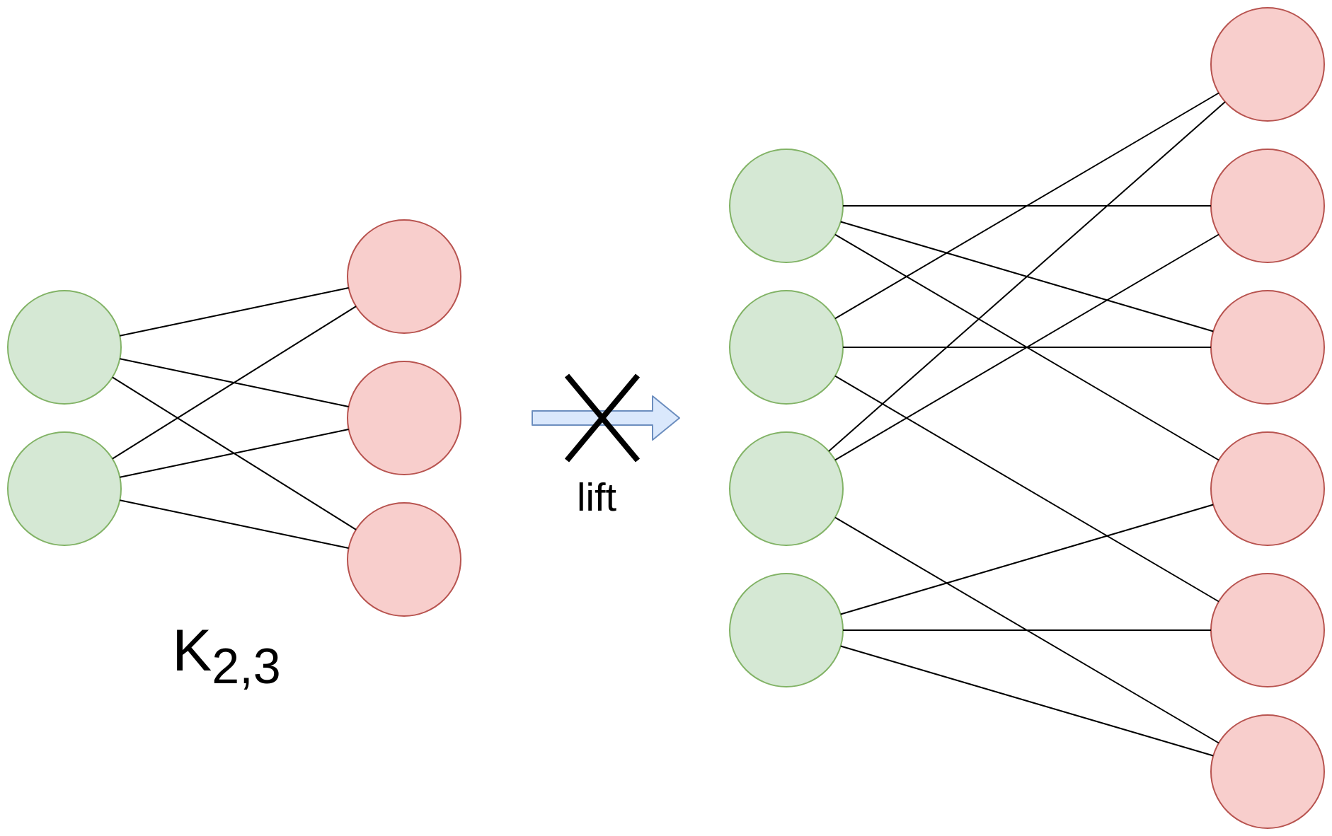
Figure 2. The $(3,2)$-bipartite, biregular graph on the right is not a 2-lift of $K_{2,3}$. Every pair of left vertices shares a neighbor on the right.

Since the eventual goal of any argument based on lifts that also applies to the configuration model would have to show that almost all bipartite, biregular graphs can be obtained by lifting and are sampled asymptotically uniformly from the lift model, the above considerations suggest this argument would be highly non-trivial. We in fact doubt such an argument can be made. Intuitively, in the configuration model edges occur “nearly independently,” whereas for random lifts there are strong dependencies due to the fact that many edges are not allowed; see Bordenave (2015).

1.3. Structure of the paper

Briefly, we now lay out the method of proof that the bipartite, biregular random graph is Ramanujan. The proof outline is given in detail in Section 5.1, after some important preliminary terms and definitions given in Section 4. The bulk of our work builds to Theorem 3, which is actually a bound on the second eigenvalue of the non-backtracking matrix $B$, as explained in Section 2. The Ramanujan bound on the second eigenvalue of $A$ then follows as Theorem 4. As a side result, we find that row- and column-regular, rectangular matrices (the off-diagonal block $X$ of the adjacency matrix in Eqn. (1)) with aspect ratio smaller than one ($d_{1}\neq d_{2}$) have full rank with high probability.

To find the second eigenvalue of $B$, we subtract from it a matrix $S$ that is formed from the leading eigenvectors, and examine the spectral norm of the “almost-centered” matrix $\bar{B}=B-S$. We then proceed to use the trace method to bound the spectral norm of the matrix $\bar{B}^{\ell}$ by its trace. However, since $\bar{B}$ is not positive definite, this leads us to consider

$$\mathbb{E}\left(\|\bar{B}^{\ell}\|^{2k}\right)\leq\mathbb{E}\left(\mathrm{Tr}\left((\bar{B}^{\ell})(\bar{B}^{\ell})^{*}\right)^{k}\right)~{}.$$

On the right hand side, the terms in $\bar{B}^{\ell}$ refer to circuits built up of $2k$ segments, each of length $\ell+1$, since an entry $B_{ef}$ is a walk on two edges. Because the degrees are bounded, it turns out that, for $\ell=O(\log(n))$, the depth $\ell$ neighborhoods of every vertex contain at most one cycle—they are “tangle-free.” Thus, we can bound the trace by computing the expectation of the circuits that contribute, along with an upper bound on their multiplicity, taking each segment to be $\ell$-tangle-free.

Finally, to demonstrate the usefulness of the spectral gap, we highlight three applications of our bound. In Section 6, we show a community detection application. Finding communities in networks is important for the areas of social network, bioinformatics, neuroscience, among others. Random graphs offer tractable models to study when detection and recovery are possible.

We show here how our results lead to community detection in regular stochastic block models with arbitrary numbers of groups, using a very general theorem by Wan and Meilă (2015). Previously, Newman and Martin (2014) studied the spectral density of such models, and the community detection problem of the special case of two groups was previously studied by Brito, Dumitriu, Ganguly, Hoffman, and Tran (2015) and Barucca (2017).

In Section 7, we examine the application to linear error correcting codes built from sparse expander graphs. This concept was first introduced by Gallager (1962) who explicitly used random bipartite biregular graphs. These “low density parity check” codes enjoyed a renaissance in the 1990s, when people realized they were well-suited to modern computers. For an overview, see Richardson and Urbanke (2003, 2008). Our result yields an explicit lower bound on the minimum distance of such codes, i.e. the number of errors that can be corrected.

The final application, in Section 8, leads to generalized error bounds for matrix completion. Matrix completion is the problem of reconstructing a matrix from observations of a subset of entries. Heiman, Schechtman, and Shraibman (2014) gave an algorithm for reconstruction of a square matrix with low complexity as measured by a norm $\gamma_{2}$, which is similar to the trace norm (sum of the singular values, also called the nuclear norm or Ky Fan $n$-norm). The entries which are observed are at the nonzero entries of the adjacency matrix of a bipartite, biregular graph. The error of the reconstruction is bounded above by a factor which is proportional to the ratio of the leading two eigenvalues, so that a graph with larger spectral gap has a smaller generalization error. We extend their results to rectangular graphs, along the way strengthening them by a constant factor of two. The main result of the paper gives an explicit bound in terms of $d_{1}$ and $d_{2}$.

As this paper was being prepared for submission, we became aware of the work of Deshpande, Montanari, O’Donnell, Schramm, and Sen (2018). In their interesting paper, they use the smallest positive eigenvalue of a random bipartite lift to study convex relaxation techniques for random not-all-equal-3SAT problems. It seems that our main result addresses the configuration model version of this constraint satisfaction problem, the first open question listed at the end of Deshpande, Montanari, O’Donnell, Schramm, and Sen (2018).

2. Non-backtracking matrix $B$

Given $G\sim\mathcal{G}(n,m,d_{1},d_{2})$, we define the non-backtracking operator $B$. This operator is a linear endomorphism of $\operatorname{\mathbb{R}}^{|\vec{E}|}$, where $\vec{E}$ is the set of oriented edges of $G$ and $|\vec{E}|=2|E|$. Throughout this paper, we will use $V(H)$, $E(H)$, and $\vec{E}(H)$ to denote the vertices, edges, and oriented or directed edges of a graph, subgraph, or path $H$. For oriented edges $e=(u,v)$, where $u$ and $v$ are the starting and ending vertices of $e$, and $f=(s,t)$, define:

$$B_{ef}=\begin{cases}1,&\textrm{if $v=s$ and $u\neq t$};\\ 0,&\textrm{otherwise}.\end{cases}$$

We order the elements of $\vec{E}$ as $\{e_{1},e_{2},\cdots,e_{2|E|}\}$, so that the first $|E|$ have end point in the set $V_{2}$. In this way, we can write

$$B=\left(\begin{array}[]{cc}0&B^{(12)}\\ B^{(21)}&0\end{array}\right).$$

for $|E|\times|E|$ matrices $B^{(12)}$ and $B^{(21)}$ with entries equal to $0$ or $1$.

We are interested in the spectrum of $B$. Denote by $\mathbf{1}_{\alpha}$ the vector with first $|E|$ coordinates equal to $1$ and the last $|E|$ equal to $\alpha=\sqrt{d_{1}-1}/\sqrt{d_{2}-1}$. We can check that

$$B\mathbf{1}_{\alpha}=B^{*}\mathbf{1}_{\alpha}=\lambda\mathbf{1}_{\alpha}$$

for $\lambda=\sqrt{(d_{1}-1)(d_{2}-1)}$. By the Perron-Frobenius Theorem, we conclude that $\lambda_{1}=\lambda$ and the associated eigenspace has dimension one. Also, one can check that if $\lambda$ is an eigenvalue of $B$ with eigenvector $v=(v_{1},v_{2})$, $v_{i}\in\mathbb{R}^{|E|}$ then $-\lambda$ is also an eigenvalue with eigenvector $v^{\prime}=(-v_{1},v_{2})$. Thus, $\sigma(B)=-\sigma(B)$ and $\lambda_{2|E|}=-\lambda_{1}$.

2.1. Connecting the spectra of $A$ and $B$

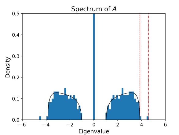
Figure 3. Example spectra for a sample graph $G\sim\mathcal{G}(120,280,7,3)$. Left, we depict the spectrum of the adjacency matrix $A$. The dash-dotted line marks the leading eigenvalue, while the dashed line marks our bound for the second eigenvalue, Theorem (4). The Marc̆enko-Pastur limiting spectral density, Eqn. (3), is shown in black. Right, we depict the spectrum of the non-backtracking matrix $B$ for the same graph. Each eigenvalue is shown as a transparent orange circle, the leading eigenvalues are marked with blue crosses, and the eigenvalues arising from zero eigenvalues of $A$ are marked with blue stars. Our main result, Theorem 3, proves that with high probability the non-leading eigenvalues are inside, on, or very close to the black dashed circle. In this case there are 8 outliers of the circle, which arise from 2 pairs of eigenvalues below and above the Marc̆enko-Pastur bulk.

Understanding the spectrum of $B$ turns out to be a challenging question. A useful result in this direction is the following theorem proved by Bass (1992), and subsequently in Watanabe and Fukumizu (2009) and Kotani and Sunada (2000); see also Theorem 3.3 in Angel, Friedman, and Hoory (2015).

Theorem 1 (Ihara-Bass formula).

Let $G=(V,E)$ be any finite graph and $B$ be its non-backtracking matrix. Then

$$\mathrm{det}(B-\lambda I)=(\lambda^{2}-1)^{|E|-|V|}\mathrm{det}(D-\lambda A+\lambda^{2}I),$$

where $D$ is the diagonal matrix with $D_{vv}=d_{v}-1$ and $A$ is the adjacency matrix of $G$.

We use the Ihara-Bass formula to analyze the relationship of the spectrum of $B$ to the spectrum of $A$ in the case of a bipartite biregular graph. It will turn out that this relationship can be completely unpacked. From Theorem 1, we get that

$$\sigma(B)=\{\pm 1\}\bigcup\{\lambda:~{}D-\lambda A+\lambda^{2}I~{}\textrm{is not invertible}\}.$$

Note that there are precisely $2(m+n)$ eigenvalues of $B$ that are determined by $A$, and that $\lambda=0$ is not in the spectrum of $B$, since the graph has no isolated vertices ($\det(D)\neq 0$).

We use the special structure of $G$ to get a more precise description of $\sigma(B)$. The matrices $A$ and $D$ are equal to:

$$A=\left(\begin{array}[]{cc}0&X\\ X^{*}&0\end{array}\right),\ \ D=\left(\begin{array}[]{cc}(d_{1}-1)I_{n}&0\\ 0&(d_{2}-1)I_{m}\end{array}\right),$$

where $I_{k}$ is the $k\times k$ identity matrix. Let $\lambda\in\sigma(B)\backslash\{-1,1\}$. Then there exists a nonzero vector $v$ such that

$$(D-\lambda A+\lambda^{2}I)v=0.$$

Writing $v=(v_{1},v_{2})$ with $v_{1}\in\mathbb{C}^{n}$, $v_{2}\in\mathbb{C}^{m}$, we obtain:

(4) $$Xv_{2} = \frac{d_{1}-1+\lambda^{2}}{\lambda}v_{1},$$

(5) $$X^{*}v_{1} = \frac{d_{2}-1+\lambda^{2}}{\lambda}v_{2}~{}.$$

The above imply that, provided that the right hand side is non-zero,

(6) $$\xi^{2}=\frac{(d_{1}-1+\lambda^{2})(d_{2}-1+\lambda^{2})}{\lambda^{2}}$$

is a nonzero eigenvalue of both $XX^{*}$ with eigenvector $v_{1}$ and $X^{*}X$, with eigenvector $v_{2}$. We can rewrite Eqn. (6) as

(7) $$\lambda^{4}-(\xi^{2}-d_{1}-d_{2}+2)\lambda^{2}+(d_{1}-1)(d_{2}-1)=0~{}.$$

We will now detail how the eigenvalues of $A$ (denoted $\xi$ here) map to eigenvalues of $B$ and vice-versa. Let us examine the special case $\xi=0$. Assume $n\leq m$ for simplicity. Assume that the rank of $X$ is $r$. Then $X$ has $m-r$ independent vectors in its nullspace. Let $u$ be one such vector. Now, if we pick $v_{2}=u$, $v_{1}=0$, and $\lambda=\pm i\sqrt{d_{2}-1}$, Eqns. (4) and (5) are satisfied. Hence, $\pm i\sqrt{d_{2}-1}$ are eigenvalues of $B$, both with multiplicity $m-r$.

Since the rank of $X$ is $r$, it follows that the nullity of $X^{*}$ is $n-r$, so there are $n-r$ independent vectors $w$ for which $X^{*}w=0$. Now, note that picking $v_{1}=w$, $v_{2}=0$, and $\lambda=\pm i\sqrt{d_{1}-1}$, we satisfy Eqns. (4) and (5). Thus, $\pm i\sqrt{d_{1}-1}$ are eigenvalues of $B$, both with multiplicity $n-r$.

The remaining $4r$ eigenvalues of $B$ determined by $A$ come from nonzero eigenvalues of $A$. For each $\xi^{2}$ with $\xi$ a nonzero eigenvalue of $A$, we will have precisely $4$ complex solutions to Eqn. (6). Since there are $2r$ such eigenvalues, coming in pairs $\pm\xi$, they determine a total of $4r$ eigenvalues of $B$, and the count is complete. To summarize the discussion above, we have the following Lemma:

Lemma 2.

Any eigenvalue of $B$ belongs to one of the following categories:

1. $\pm 1$ are both eigenvalues with multiplicities $|E|-|V|=nd_{1}-m-n$,

2. $\pm i\sqrt{d_{1}-1}$ are eigenvalues with multiplicities $m-r$, where $r$ is the rank of the matrix $X$,

3. $\pm i\sqrt{d_{2}-1}$ are eigenvalues with multiplicities $r$, and

4. every pair of non-zero eigenvalues $(-\xi,\xi)$ of $A$ generates exactly $4$ eigenvalues of $B$.

3. Main result

We spend the bulk of this paper in the proof of the following:

Theorem 3.

If $B$ is the non-backtracking matrix of a bipartite, biregular random graph $G\sim\mathcal{G}(n,m,d_{1},d_{2})$, then its second largest eigenvalue

$$|\lambda_{2}(B)|\leq((d_{1}-1)(d_{2}-1))^{1/4}+\epsilon_{n}$$

asymptotically almost surely, with $\epsilon_{n}\to 0$ as $n\to\infty$. Equivalently, there exists a sequence $\epsilon_{n}\rightarrow 0$ as $n\rightarrow\infty$ so that

$$\mathbb{P}\left[|\lambda_{2}(B)|-((d_{1}-1)(d_{2}-1))^{1/4}>\epsilon_{n}\right]\rightarrow 0~{}~{}\mbox{as}~{}~{}n\rightarrow\infty~{}.$$

Remark.

For the random lift model, Theorem 3 was proved by Bordenave (2015), which applies to random bipartite graphs only when $d_{1}=d_{2}=d$ as discussed in section 1.2.

We combine Theorems 1 and 3 to prove our main result concerning the spectrum of $A$.

Theorem 4 (Spectral gap).

Let $A=\left(\begin{array}[]{cc}0&X\\ X^{*}&0\end{array}\right)$ be the adjacency matrix of a bipartite, biregular random graph $G\sim\mathcal{G}(n,m,d_{1},d_{2})$. Without loss of generality, assume $d_{1}\geq d_{2}$ or, equivalently, $n\leq m$. Then:

1. Its second largest eigenvalue $\eta=\lambda_{2}(A)$ satisfies

   $$\eta\leq\sqrt{d_{1}-1}+\sqrt{d_{2}-1}+\epsilon_{n}^{\prime}$$

   asymptotically almost surely, with $\epsilon_{n}^{\prime}\to 0$ as $n\to\infty$.

2. Its smallest positive eigenvalue $\eta^{+}_{\rm min}=\min(\{\lambda\in\sigma(A):\lambda>0\})$ satisfies

   $$\eta_{\rm min}^{+}\geq\sqrt{d_{1}-1}-\sqrt{d_{2}-1}-\epsilon_{n}^{\prime\prime}$$

   asymptotically almost surely, with $\epsilon_{n}^{\prime\prime}\to 0$ as $n\to\infty$. (Note that this will be almost surely positive if $d_{1}>d_{2}$; no further information is gained if $d_{1}=d_{2}$.)

3. If $d_{1}\neq d_{2}$, the rank of $X$ is $n$ with high probability.

Remark.

Since the first draft of this work came out, considerable advances haven been made regarding the question of singularity of random regular graphs. It was conjectured in Costello and Vu (2008) that, for $3\leq d\leq n-3$, the adjacency matrix of uniform $d$-regular graphs is not singular with high probability as $n$ grows to infinity. For directed $d$-regular graphs and growing $d$, this is now known to be true, following the results of Cook (2017) and Litvak, Lytova, Tikhomirov, Tomczak-Jaegermann, and Youssef (2016, 2017). For constant degree $d$, Huang (2018a, b) proved the asymptotic non-singularity of the adjacency matrix for both undirected and directed $d-$regular graphs. The last case can be interpreted as singularity of the adjacency matrix of random $d-$regular bipartite graph. To the best of our knowledge, Theorem 4(iii) is the first result concerning the rank of rectangular random matrices with $d_{1}$ nonzero entries in each row and $d_{2}$ in each column.

Remark.

The analysis of the Ihara-Bass formula for Markov matrices of bipartite biregular graph appeared before in Kempton (2016). We have independently proven Lemma 2 and extracted from it more information than is given in Kempton (2016), including Theorem 4(iii).

Proof.

Eqn. (7), describing those eigenvalues of $B$ which are neither $\pm 1$ and do not correspond to $0$ eigenvalues of $A$, is equivalent to

(8) $$0=x^{2}+\alpha\beta-(y-\alpha-\beta)x,$$

where $x=\lambda^{2}$, $y=\xi^{2}$, $\alpha=d_{1}-1$, and $\beta=d_{2}-1$. A simple discriminant calculation and analysis of Eqn. (8), keeping in mind that $y\neq 0$, leads to a number of cases in terms of $y$:

1. $y\in((\sqrt{\alpha}-\sqrt{\beta})^{2},(\sqrt{\alpha}+\sqrt{\beta})^{2})$, i.e. roughly speaking, $\eta$ is in the bulk, means that $x$ is on the circle of radius $\sqrt{\alpha\beta}$ and the corresponding pair of eigenvalues $\lambda$ are on a circle of radius $(\alpha\beta)^{1/4}$.

2. $y\in(0,(\sqrt{\alpha}-\sqrt{\beta})^{2}]$ means that $x$ is real and negative, so $\lambda$ is purely imaginary.

   In this case, one may also show that the smaller of the two possible values for $x$ is increasing as a function of $y$ and $x_{-}\in(-\alpha,-\sqrt{\alpha\beta}]$. The larger of the two values of $x$ is decreasing and $x_{+}\in[-\sqrt{\alpha\beta},-\beta)$. Correspondingly, the largest in absolute value that $\lambda$ could be in this case is $\pm i\alpha^{1/4}=\pm i(d_{1}-1)^{1/4}$.

3. $y\geq(\sqrt{\alpha}+\sqrt{\beta})^{2}$ means that both solutions $x_{\pm}$ are real, and the larger of the two is larger than $\sqrt{\alpha\beta}$.

Note that Eqn. 8 shows there is a continuous dependence between $x$ and $y$, and consequently between $\xi$ and $\lambda$. Putting these cases together with Lemma 2, a few things become apparent:

1. $\xi>\sqrt{d_{1}-1}+\sqrt{d_{2}-1}$ means that $\lambda>((d_{1}-1)(d_{2}-1))^{1/4}$.

2. $|\lambda_{2}|\leq((d_{1}-1)(d_{2}-1))^{1/4}+\epsilon$ implies that all eigenvalues except for the largest two will be either $0$, or in a small neighborhood $[\sqrt{\alpha}-\sqrt{\beta}-\delta,\sqrt{\alpha}+\sqrt{\beta}+\delta]$ of the bulk, with $\delta$ small if $\epsilon$ is small since the dependence of $\delta$ on $\epsilon$ can be deduced from Eqn. 8.

3. $|\lambda_{2}|\leq((d_{1}-1)(d_{2}-1))^{1/4}+\epsilon$ with high probability implies that if $d_{1}\neq d_{2}$, $r=n$ with high probability. Otherwise, we would have eigenvalues of $B$ with absolute value $\sqrt{d_{1}-1}$ and this is larger than $((d_{1}-1)(d_{2}-1))^{1/4}$.

This completes the proof, with results (i) and (ii) following from the point 2 and (iii) following from point 3. ∎

In Fig. 3, we depict the spectra of $A$ and $B$ for a sample graph $G\sim\mathcal{G}(120,280,7,3)$. Looking at the non-backtracking spectrum, we observe the two leading eigenvalues $\pm\sqrt{(d_{1}-1)(d_{2}-1)}$ (blue crosses) outside the circle of radius $((d_{1}-1)(d_{2}-1))^{1/4}$ along with a number of zero eigenvalues (black dots). There are also multiple purely imaginary eigenvalues which can arise from $|\xi|\in(0,\sqrt{d_{1}-1}-\sqrt{d_{2}-1}]$ as well as $\xi=0$. However, due to Theorem 4, only the smaller of $i\sqrt{d_{1}-1}$ and $i\sqrt{d_{2}-1}$ is observed with non-negligible probability, implying that $X$ has rank $r=n$ with high probability (shown as blue stars). Furthermore, we observe two pairs of real eigenvalues of $B$ which are connected to a pair of eigenvalues of $A$ from “above” the bulk, as well as two pairs of imaginary eigenvalues of $B$ which are connected to a pair of eigenvalues of $A$ from “below” the bulk.

4. Preliminaries

We describe the standard configuration model for constructing such graphs. We then define the “tangle-free” property of random graphs. Since small enough neighborhoods are tangle-free with high probability, we only need to count tangle-free paths when we eventually employ the trace method.

4.1. The configuration model

The configuration or permutation model is a practical procedure to sample random graphs with a given degree distribution. Let us recall its definition for bipartite biregular graphs. Let $V_{1}=\{v_{1},v_{2},\dots,v_{n}\}$ and $V_{2}=\{w_{1},w_{2},\dots,w_{m}\}$ be the vertices of the graph. We define the set of half edges out of $V_{1}$ to be the collection of ordered pairs

$$\vec{E}_{1}=\{(v_{i},j)~{}\mbox{for $1\leq i\leq n$ and $1\leq j\leq d_{1}$}\}$$

and analogously the set of half edges out of $V_{2}$:

$$\vec{E}_{2}=\{(w_{i},j)~{}\mbox{for $1\leq i\leq m$ and $1\leq j\leq d_{2}$}\},$$

see Figure 1. Note that $|\vec{E}_{1}|=|\vec{E}_{2}|=nd_{1}=md_{2}=|E|$. To sample a graph, we choose a random permutation $\pi$ of $[nd_{1}]$. We put an edge between $v_{i}$ and $w_{j}$ in the $G$ whenever

$$\pi((i-1)d_{1}+s)=(j-1)d_{2}+t$$

for any pair of values $1\leq s\leq d_{1}$, $1\leq t\leq d_{2}$. For specific half edges $e=(v_{i},j)$ and $f=(w_{s},t)$, we use the notation $\pi(e)=f$ as shorthand for $\pi((i-1)d_{1}+j)=(s-1)d_{2}+t$ and say that “$e$ matches to $f$.”

The graph obtained may not be simple, since multiple half edges may be matched between any pair of vertices. However, conditioning on a simple graph outcome, the distribution is uniform in the set of all simple bipartite biregular graphs. Furthermore, for fixed $d_{1},d_{2}$ and $n,m\to\infty$, the probability of getting a simple graph is bounded away from zero (Bollobás, 2001).

Consider the random $B\in\operatorname{\mathbb{R}}^{2|E|\times 2|E|}$ whose first $|E|$ rows are indexed by the elements of $\vec{E}_{1}$ and the last $|E|$ rows are indexed by those of $\vec{E}_{2}$, in lexicographic order. Columns are indexed in the same way. Entry $B_{ef}$ with $e=(v_{i},j)\in\vec{E}_{1}$ and $f=(w_{s},t)\in\vec{E}_{2}$ is defined as

$$B_{ef}=\begin{cases}1,&\mbox{if $\pi(e)=f^{\prime}=(w_{s},t^{\prime})$ and $t^{\prime}\neq t$};\\ 0,&\textrm{otherwise}.\end{cases}$$

This defines the upper half of $B$. We define the lower half similarly, by putting

$$B_{fe}=\begin{cases}1,&\textrm{if $\pi^{-1}(f)=e^{\prime}=(v_{i},j^{\prime})$ and $j^{\prime}\neq j$};\\ 0,&\textrm{otherwise}.\end{cases}$$

This is the same definition used in Bordenave (2015). In words, it says that the directed edge given by $e$ followed by the directed edge given by $f$ are connected by some half edge $f^{\prime}=(w_{s},t^{\prime})$, and the path they form does not backtrack. This is therefore the same matrix introduced in Section 2, ordered according to the half edges. Notice that the randomness comes from the matching only.

We consider two symmetric matrices $M=M(\pi)$ and $N$, indexed the same as $B$, and defined by:

$$M_{ef}=1_{\{\pi(e)=f\}}\mbox{ and }M_{fe}=1_{\{\pi^{-1}(f)=e\}}~{}\mbox{ for $e\in\vec{E}_{1}$ and $f\in\vec{E}_{2}$}$$

and

$$N_{gh}=1_{\{u=v\mbox{ and }i\neq j\}}~{}\mbox{ for $g=(u,i),h=(v,j)\in\vec{E}_{1}\cup\vec{E}_{2}$}.$$

We see that a term like $M_{eg}N_{gf}$ corresponds to $M$ matching the directed edge $e$ to $g$ by $\pi$, and $N$ taking us out of the vertex of $g$ along the directed edge $f$, which is different from $g$. Thus the rule of matrix multiplication means that

(9) $$B=MN.$$

This equality will be useful in Section 5.2 when working with products of the matrix $B$.

4.2. Tangle-free paths

Sparse random graphs, including bipartite graphs, have the important property of being “tree-like” in the neighborhood of a typical vertex. Formally, consider a vertex $v\in V_{1}\cup V_{2}$. For a natural number $\ell$, we define the ball of radius $\ell$ centered at $v$ to be:

$$B_{\ell}(v)=\{w\in V_{1}\cup V_{2}:~{}d_{G}(v,w)\leq\ell\}$$

where $d_{G}(\cdot,\cdot)$ is the graph distance.

Definition 1.

A graph $G$ is $\ell$-tangle-free if $B_{\ell}(v)$ contains at most one cycle for any vertex $v$.

The next lemma says that most bipartite biregular graphs are $\ell$-tangle-free up to logarithmic sized neighborhoods.

Lemma 5.

Let $G\sim\mathcal{G}(n,m,d_{1},d_{2})$ be a bipartite, biregular random graph. Let $\ell<\frac{1}{8}\log_{d}(n)$, for $d=\max\{d_{1},d_{2}\}$. Then $G$ is $\ell$-tangle-free with probability at least $1-n^{-1/2}$.

Proof.

This is essentially the proof given in Lubetzky and Sly (2010), Lemma 2.1. Fix a vertex $v$. We will use the so called exploration process to discover the ball $B_{\ell}(v)$. More precisely, we order the set $\vec{E}_{1}$ lexicographically: $(v_{i},j)<(v_{i^{\prime}},j^{\prime})$ if $i\leq i^{\prime}$ and $j\leq j^{\prime}$. The exploration process reveals $\pi$ one edge at the time, by doing the following:

• A uniform element is chosen from $\vec{E}_{2}$ and it is declared equal to $\pi(1)$.

• A second element is chosen uniformly, now from the set $\vec{E}_{2}\backslash\{\pi(1)\}$ and set equal to $\pi(2)$.

• Once we have determined $\pi(i)$ for $i\leq k$, we set $\pi(k+1)$ equal to a uniform element sampled from the set $\vec{E}_{2}\backslash\{\pi(1),\pi(2),\dots,\pi(k)\}$.

We use the final $\pi$ to output a graph as we did in the configuration model. The law of these graphs is the same. With the exploration process, we expose first the neighbors of $v$, then the neighbors of these vertices, and so on. This breadth-first search reveals all vertices in $B_{k}(v)$ before any vertices in $B_{j>k}(v)$. Note that, although our bound is for the family $\mathcal{G}(n,m,d_{1},d_{2})$, the neighborhood sizes are bounded above by those of the $d$-regular graph with $d=\max(d_{1},d_{2})$.

Consider the matching of half edges attached to vertices in the ball $B_{i}(v)$ at depth $i$ (thus revealing vertices at depth $i+1$). In this process, we match a maximum $m_{i}\leq d^{i+1}$ pairs of half edges total. Let $\mathcal{F}_{i,k}$ be the filtration generated by matching up to the $k$th half edge in $B_{i}(v)$, for $1\leq k\leq m_{i}$. Denote by $A_{i,k}$ the event that the $k$th matching creates a cycle at the current depth. For this to happen, the matched vertex must have appeared among the $k-1$ vertices already revealed at depth $i+1$. The number of unmatched half edges is at least $nd-2d^{i+1}$. We then have that:

$$\mathbb{P}(A_{i,k})\leq\frac{(k-1)(d-1)}{nd-2d^{i+1}}\leq\frac{(d-1)m_{i}}{(1-2d^{i+1}n^{-1})nd}\leq\frac{m_{i}}{n}.$$

So, we can stochastically dominate the sum

$$\sum_{i=1}^{\ell-1}\sum_{k=1}^{m_{i}}A_{i,k}$$

by $Z\sim\mathrm{Bin}\left(d^{\ell+1},\ n^{-1}d^{\ell}\right)$. So the probability that $B_{\ell}(v)$ is $\ell$-tangle-free has the bound:

$$\mathbb{P}(\mbox{$B_{\ell}(v)$ is not $\ell$-tangle-free})=\mathbb{P}\left(\sum_{i=1}^{\ell-1}\sum_{k=1}^{m_{i}}A_{i,k}>1\right)\leq\mathbb{P}(Z>1)=O\left(\frac{d^{4\ell+1}}{n^{2}}\right)=O\left(n^{-3/2}\right),$$

which follows using that $\ell=c\log_{d}n$ with $c<1/8$. The Lemma follows by taking a union bound over all vertices. ∎

5. Proof of Theorem 3

5.1. Outline

We are now prepared to explain the main result. To study the second largest eigenvalue of the non-backtracking matrix, we examine the spectral radius of the matrix obtained by subtracting off the dominant eigenspace. We use for this:

Lemma 6 (Bordenave, Lelarge, and Massoulié (2015), Lemma 3).

Let $T$ and $R$ be matrices such that $\mathrm{Im}(T)\subset\mathrm{Ker}(R)$, $\mathrm{Im}(T^{*})\subset\mathrm{Ker}(R)$. Then all eigenvalues $\lambda$ of $T+R$ that are not eigenvalues of $T$ satisfy:

$$|\lambda|\leq\max_{x\in\mathrm{Ker}(T)}\frac{\|(T+R)x\|}{\|x\|}.$$

Throughout the text, $\|\cdot\|$ is the spectral norm for matrices and $\ell^{2}$-norm for vectors. Recall that the leading eigenvalues of $B$, in magnitude, are $\lambda_{1}=\sqrt{(d_{1}-1)(d_{2}-1)}$ and $\lambda_{2|E|}=-\lambda_{1}$ with corresponding eigenvectors $\mathbf{1}_{\alpha}$ and $\mathbf{1}_{-\alpha}$. Applying Lemma 6 with $T=\frac{\lambda_{1}^{\ell}}{\mathbf{1}_{\alpha}^{*}\mathbf{1}_{\alpha}}(\mathbf{1}_{\alpha}\mathbf{1}_{\alpha}^{*}+(-1)^{\ell}\mathbf{1}_{-\alpha}\mathbf{1}_{-\alpha}^{*})$ and $R=B^{\ell}-T$, we get that

(12) $$\lambda_{2}(B)\leq\max_{\footnotesize\begin{array}[]{c}x\in\mathrm{Ker}(T)\\ \|x\|=1\end{array}}\left(\|B^{\ell}x\|\right)^{1/\ell}.$$

It will be important later to have a more precise description of the set $\mathrm{Ker}(T)$. It is not hard to check that

$$\mathrm{Ker}(T) =\{x:~{}\langle x,\mathbf{1}_{\alpha}\rangle=\langle x,\mathbf{1}_{-\alpha}\rangle=0\}$$

$$=\{(v,w)\in\mathbb{R}^{2|E|}:~{}\langle v,\mathbf{1}\rangle=\langle w,\mathbf{1}\rangle=0\}.$$

In the last line, the vectors $v$, $w$ and $\mathbf{1}$ are $|E|-$dimensional, and $\mathbf{1}$ is the vector of all ones.

In order to use Eqn. 12, we must bound $\|B^{\ell}x\|$ for large powers $\ell$ and $x\in\mathrm{Ker}(T)$. This amounts to counting the contributions of certain non-backtracking walks. We will use the tangle free property in order to only count $\ell$-tangle-free walks. We break up $B^{\ell}$ into two parts in Section 5.2, an “almost” centered matrix $\bar{B}^{\ell}$ and the remainder $\sum_{j}R^{\ell,j}$, and we bound each term independently.

To compute these bounds, we need to count the contributions of many different non-backtracking walks. We will use the trace technique, so only circuits which return to the starting vertex will contribute. In Section 5.3, we compute the expected contribution of products of $B$ along such circuits, employing a result from Bordenave (2015).

Section 5.4 covers the combinatorial component of the proof. The total contributions $\|B^{\ell}x\|$ come from many non-backtracking circuits of different flavors, depending on their number of vertices, edges, cycles, etc. Each circuit is broken up into $2k$ segments of tangle-free walks of length $\ell$. We need to compute not only the expectation along the circuit, but also upper-bound the number of circuits of each flavor. We introduce an injective encoding of such circuits that depends on the number of vertices, length of the circuit, and, crucially, the tree excess of the circuit. An important part of these calculations is to keep track of the imbalance between left and right vertices visited in the circuit, since this controls the powers of $d_{1}$ and $d_{2}$ in the result.

Finally, in Section 5.8 we put all of these ingredients together and use Markov’s inequality to bound each matrix norm with high probability. We find that $\|\bar{B}^{\ell}\|$ contributes a factor that goes as $((d_{1}-1)(d_{2}-1))^{\ell/4}$, whereas $\|R^{\ell,j}\|$ contributes only a factor of $(d-1)^{\ell}/n$, up to polylogarithmic factors in $n$. Thus, the main contribution to the circuit counts comes from the mean and, in fact, comes from circuits which are exactly trees traversed forwards and backwards. Interestingly, this is analogous to what happens when using the trace method on random matrices of independent entries.

In the proof, we are forced to consider tangled paths but which are built up of tangle-free components. This delicate issue was first made clear by Friedman (2004) who introduced the idea of tangles and a “selective trace.” Bordenave, Lelarge, and Massoulié (2015), who we follow closely in this part of our analysis, also has a good discussion of these issues and their history. We use the fact that

(13) $$\mathbb{E}\left(\|\bar{B}^{\ell}\|^{2k}\right)\leq\mathbb{E}\left(\mathrm{Tr}\left[\left((\bar{B}^{\ell})(\bar{B}^{\ell})^{*}\right)^{k}\right]\right),$$

and so deal with circuits built up of $2k$ segments which are $\ell$-tangle-free. Notice that the first segment comes from $\bar{B}^{\ell}$, the second from $(\bar{B}^{\ell})^{*}$, etc. Because of this, the directionality of the edges along each segment alternates. See Figure 4 for an illustration of a path which contributes for $k=2$ and $\ell=2$. Also, while each segment is $\ell$-tangle-free, the overall circuit may be tangled.

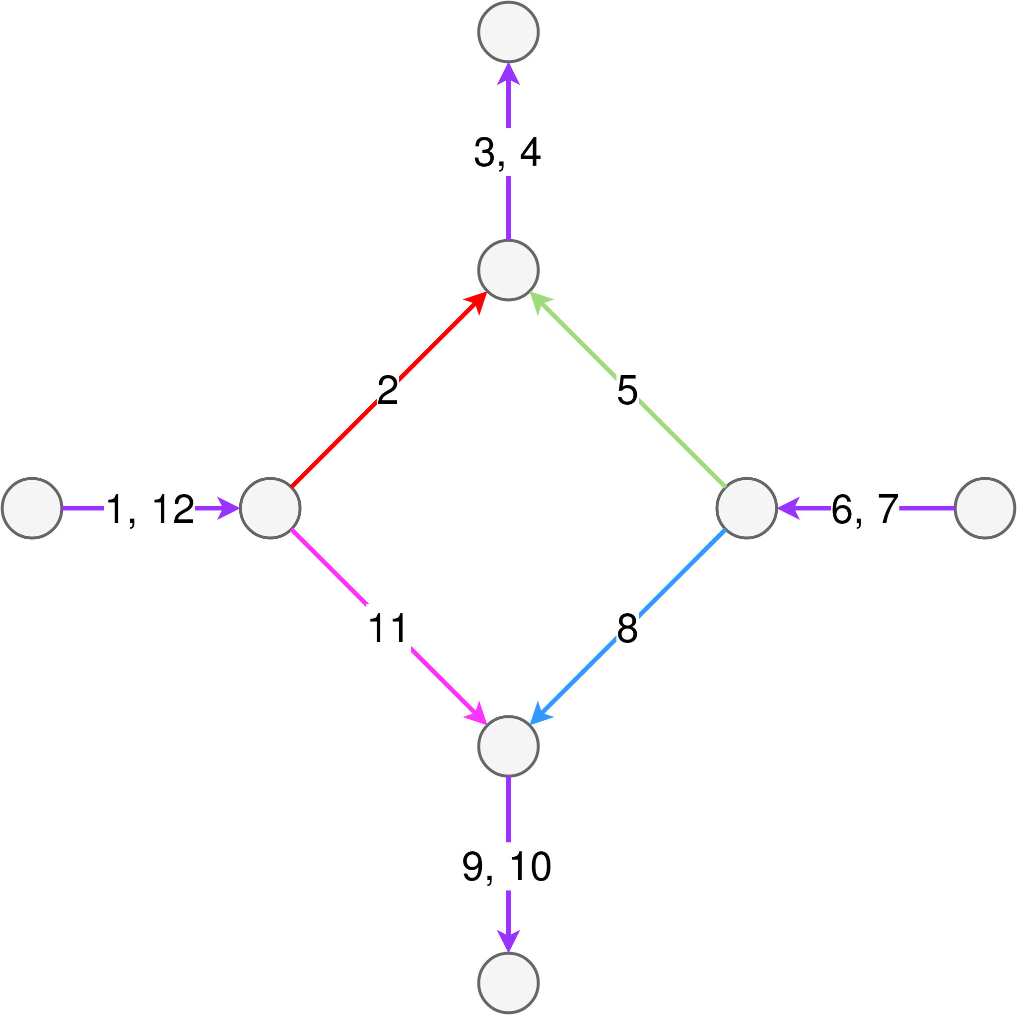
Figure 4. An example circuit that contributes to the trace in Eqn. (13), for $k=2$ and $\ell=2$. Edges are numbered as they occur in the circuit. Each segment $\{\gamma_{i}\}_{i=1}^{4}$ is of length $\ell+1=3$ and made up of edges $3(i-1)+1$ through $3i$. The last edge of each $\gamma_{i}$ is the first edge of $\gamma_{i+1}$, and these are shown in purple. Every path $\gamma_{i}$ with $i$ even follows the edges backwards due to the matrix transpose. However, this detail turns out not to make any difference since the underlying graph is undirected. Our example has no cycles in each segment for clarity, but, in general, each segment can have up to one cycle, and the overall circuit may be tangled.

5.2. Matrix decomposition

We start this section by defining the set of paths that will be relevant to bound the norm of $\|\bar{B}^{\ell}\|$. We closely follow Bordenave (2015).

Definition 2.

Define $\Gamma^{\ell}_{ef}$ to be the set of all non-backtracking paths of $2\ell+1$ half edges, starting at $e$ and ending at $f$. A path in this set will be denoted by $\gamma=(e_{1},e_{2},\dots,e_{2\ell},e_{2\ell+1})$, where $e_{1}=e$ and $e_{2\ell+1}=f$. The non-backtracking property means that, for all $1\leq i\leq\ell$, $e_{2i}$ and $e_{2i+1}$ share the same vertex but $e_{2i}\neq e_{2i+1}$. Similarly, let $\Gamma^{\ell}=\bigcup_{e,f}\Gamma^{\ell}_{ef}$.

Each path in $\Gamma^{\ell}_{ef}$ uses $2\ell+1$ half edges, corresponding to $\ell+1$ edges in the graph. To be clear, the above definition counts all possible non-backtracking sequences of half edges. These are different than the usual non-backtracking paths and do not necessarily exist in the graph. Some of these paths might backtrack along a duplicate edge which utilizes a different half edge.

We now have

(14) $$(B^{\ell})_{ef}=\sum_{\gamma\in\Gamma^{\ell}_{ef}}\prod_{t=1}^{\ell}B_{e_{2t-1}e_{2t+1}}=\sum_{\gamma\in\Gamma^{\ell}_{ef}}\prod_{t=1}^{\ell}M_{e_{2t-1}e_{2t}}N_{e_{2t}e_{2t+1}}=\sum_{\gamma\in\Gamma^{\ell}_{ef}}\prod_{t=1}^{\ell}M_{e_{2t-1}e_{2t}}$$

where we used Eqn. 9 and the fact that $\Gamma^{\ell}_{ef}$ is non-backtracking, so $N_{e_{2t}e_{2t+1}}=1$.

Recall that we will use Eqn. (12) and Lemma 6 to bound $\lambda_{2}$. Denote by $\bar{B}$ the matrix with entries equal to $\bar{B}=B-S$, where

$$S=\frac{1}{|E|}\left(\begin{array}[]{cc}0&(d_{2}-1)\mathbf{1}\mathbf{1}^{*}\\ (d_{1}-1)\mathbf{1}\mathbf{1}^{*}&0\end{array}\right).$$

Note that $\bar{B}$ is an almost centered version of $B$, and $\mathrm{Ker}(S)=\mathrm{Ker}(T)=\mathrm{span}(\mathbf{1}_{\alpha},\mathbf{1}_{-\alpha})$, where $T$ is the matrix from Lemma 6. To apply the lemma, we wish to get an expression like Eqn. (14) for $\bar{B}^{\ell}$. To do so, we write:

$$\bar{B}=B-S=MN-S=(M-S^{\prime})N$$

the above matrix equation in the unknown $S^{\prime}$ can be solved by simple manipulations. We get

$$S^{\prime}=\frac{1}{|E|}\left(\begin{array}[]{cc}0&\mathbf{1}\mathbf{1}^{*}\\ \mathbf{1}\mathbf{1}^{*}&0\end{array}\right).$$

Using again that $N$ is identically one over the elements of the set $\Gamma^{\ell}_{ef}$, we find a similar formula to Eqn. (14):

(15) $$(\bar{B}^{\ell})_{ef}=\sum_{\gamma\in\Gamma^{\ell}_{ef}}\prod_{t=1}^{\ell}\left(B-S\right)_{e_{2t-1}e_{2t+1}}=\sum_{\gamma\in\Gamma^{\ell}_{ef}}\prod_{t=1}^{\ell}\bar{M}_{e_{2t-1}e_{2t}},$$

where $\bar{M}=M-S^{\prime}$.

The following telescoping sum formula is a simple algebraic manipulation and appears in Massoulie (2013) and Bordenave, Lelarge, and Massoulié (2015):

$$\prod_{s=1}^{\ell}x_{s}=\prod_{s=1}^{\ell}y_{s}+\sum_{j=1}^{\ell}\prod_{s=1}^{j-1}y_{s}(x_{j}-y_{j})\prod_{t=j+1}^{\ell}x_{t}.$$

Using this, with $x_{s}=B_{e_{2s-1}e_{2s+1}}$ and $y_{s}=\bar{B}_{e_{2s-1}e_{2s+1}}$, we obtain the following relation:

(16) $$(B^{\ell})_{ef}=(\bar{B}^{\ell})_{ef}+\sum_{\gamma\in\Gamma^{\ell}_{ef}}\sum_{j=1}^{\ell}\prod_{s=1}^{j-1}\ \bar{B}_{e_{2s-1}e_{2s+1}}S_{e_{2j-1}e_{2j+1}}\prod_{t=j+1}^{\ell}B_{e_{2t-1}e_{2t+1}}.$$

This decomposition breaks the elements in $\Gamma^{\ell}_{ef}$ into two subpaths, also non-backtracking, of length $j$ and $\ell-j$, respectively.

Definition 3.

Let $F_{ef}^{\ell}\subset\Gamma^{\ell}_{ef}$ denote the subset of paths which are tangle-free, with $F^{\ell}=\bigcup_{e,f}F^{\ell}_{ef}$.

We will take the parameter $\ell$ to be small enough so that the path $\gamma$ is tangle-free with high probability. Thus the sums in Eqns. (14) or (15) need only be over the paths $\gamma\in F_{ef}^{\ell}$. However, to recover the matrices $B$ and $\bar{B}$ by rearranging Eqn. (16), we need to also count those tangle-free subpaths that arise from splitting tangled paths. While breaking a tangle-free path will necessarily give us two new tangle-free subpaths, the converse is not always true. This extra term generates a remainder that we define now.

Definition 4.

Let $T^{\ell,j}_{ef}$ be the set of non-backtracking paths containing $2\ell+1$ half edges, starting at $e$ and ending at $f$, such that overall the path is tangled but the first $2j-1$, middle three, and last $2(\ell-j)+1$ half edges form tangle-free subpaths: $\gamma=(e_{1},\ldots,e_{2\ell+1})\in T^{\ell,j}$ if and only if $\gamma^{\prime}=(e_{1},\ldots,e_{2j-1})\in F^{j-1}$, $\gamma^{\prime\prime}=(e_{2j-1},e_{2j},e_{2j+1})\in F^{1}$, and $\gamma^{\prime\prime\prime}=(e_{2j+1},\ldots,e_{2\ell+1})\in F^{\ell-j}$. Set $T^{\ell,j}=\bigcup_{e,f}T^{\ell,j}_{ef}$.

Set the remainder

$$R^{\ell,j}_{ef} =\sum_{\gamma\in T^{\ell,j}_{ef}}\sum_{j=1}^{\ell}\prod_{s=1}^{j-1}\bar{B}_{e_{2s-1}e_{2s+1}}S_{e_{2j-1}e_{2j+1}}\prod_{t=j+1}^{\ell}B_{e_{2t-1}e_{2t+1}}$$

(17) $$=\sum_{\gamma\in T^{\ell,j}_{ef}}\sum_{j=1}^{\ell}\prod_{s=1}^{j-1}\ \bar{M}_{e_{2s-1}e_{2s}}S_{e_{2j-1}e_{2j+1}}\prod_{t=j+1}^{\ell}M_{e_{2t-1}e_{2t}}.$$

Since the paths are non-backtracking, the $N$ terms are all unity.

Adding and subtracting $\sum_{j=1}^{\ell}R^{\ell,j}_{ef}$ to Eqn. (16) and rearranging the sums, we obtain

(18) $$B^{(\ell)}=\bar{B}^{(\ell)}+\sum_{j=1}^{\ell}\bar{B}^{(j)}SB^{(\ell-j)}-\sum_{j=1}^{\ell}R^{\ell,j},$$

where the matrices $B^{(\ell)}$ and $\bar{B}^{(\ell)}$ are tangle-free versions of $B^{\ell}$ and $\bar{B}^{\ell}$, i.e. element $ef$ in both matrices only counts paths $\gamma\in F_{ef}^{\ell}$. Multiplying Eqn. (18) on the right by $x\in\mathrm{Ker}(T)$ and using that $B^{(\ell-j)}x$ is also within $\mathrm{Ker}(S)$, since it is just the space spanned by the leading eigenvectors, we find that the middle term is identically zero. Thus for $x\in\mathrm{Ker}(T)$,

(19) $$\|B^{(\ell)}x\|\leq\|\bar{B}^{(\ell)}x\|+\left\|\sum_{j=1}^{\ell}R^{\ell,j}x\right\|\leq\|\bar{B}^{(\ell)}\|+\sum_{j=1}^{\ell}\|R^{\ell,j}\|.$$

5.3. Expectation bounds

Our goal is to find a bound on the expectation of certain random variables which are products of $\bar{B}_{ef}$ along a circuit. To do this, we will need to bound the probabilities of different subgraphs when exploring $G$. This requires us to introduce the concept of consistent edges and their multiplicity.

Definition 5.

Let $\gamma=(e_{1},\ldots,e_{2k})$ be a sequence of half edges of even length, with $\vec{E}(\gamma)$ its set of half edges, and $E(\gamma)=\{\{e_{2i-1},e_{2i}\}\mbox{ for $i\in[k]$}\}$ its set of edges (unordered pairs, thus undirected).

• The multiplicity of a half edge $e\in\vec{E}(\gamma)$ is $m_{\gamma}(e)=\sum_{t=1}^{2k}1_{\{e_{t}=e\}}$.

• The multiplicity of an edge $\{h_{1},h_{2}\}\in E(\gamma)$, is $m_{\gamma}(\{h_{1},h_{2}\})=\sum_{t=1}^{k}1_{\{\{e_{2t-1},e_{2t}\}=\{h_{1},h_{2}\}\}}$.

• An edge $\{h_{1},h_{2}\}$ is consistent if $m_{\gamma}(h_{1})=m_{\gamma}(h_{2})=m_{\gamma}(\{h_{1},h_{2}\})$.

Lemma 7.

Let $\gamma=(e_{1},\ldots,e_{2k})$ be a sequence of half edges of even length, with $M$ and $\bar{M}$ the matching matrix and its centered version generated by a uniform matching in the configuration model. Then for $1\leq k\leq\sqrt{|E|}$ and $0\leq t_{0}\leq k$ we have that

$$\left|\mathbb{E}\prod_{t=1}^{t_{0}}\bar{M}_{e_{2t-1}e_{2t}}\prod_{t=t_{0}+1}^{k}M_{e_{2t-1}e_{2t}}\right|\leq C\cdot 2^{b}\cdot\left(\frac{1}{|E|}\right)^{\mathscr{E}}\left(\frac{3k}{\sqrt{|E|}}\right)^{\mathscr{E}_{1}}$$

where $b=$ number of inconsistent edges of multiplicity one occuring before $t_{0}$, $\mathscr{E}_{1}=$ number of consistent edges with multiplicity one occuring before $t_{0}$, $\mathscr{E}=|E(\gamma)|$, and $C$ is a universal constant.

Proof.

Recall the form of the matrices

$$M=\left(\begin{array}[]{cc}0&M_{1}\\ M_{1}^{*}&0\end{array}\right)\quad\mbox{and}\quad\bar{M}=M-\frac{1}{|E|}\left(\begin{array}[]{cc}0&\mathbf{1}\mathbf{1}^{*}\\ \mathbf{1}\mathbf{1}^{*}&0\end{array}\right).$$

Matrix $M_{1}\in\operatorname{\mathbb{R}}^{|E|\times|E|}$ is a random permutation matrix between $nd_{1}=|E|$ and $md_{2}=|E|$ half edges. Therefore, $M_{1}$ is distributed exactly the same as a matching matrix of a random $|E|$-lift of a single edge, and the same holds for its centered version $M_{1}-\frac{1}{|E|}\mathbf{1}\mathbf{1}^{*}$. The only paths $\gamma$ that contribute in this bipartite setting must alternate between the bipartite sets and avoid the 0 blocks, otherwise the bound holds trivially. For one of these paths $\gamma$ assume, without loss of generality, that the path starts in set $V_{1}$. Then define the transformed path $\gamma^{\prime}=(e_{1}^{\prime},\ldots,e_{2k}^{\prime})=(e_{1},e_{2},e_{4},e_{3},e_{5},\ldots)$, i.e. with every other pair in $\gamma$ in reverse order. Note that

(20) $$\prod_{t=1}^{t_{0}}\bar{M}_{e_{2t-1}e_{2t}}\prod_{t=t_{0}+1}^{k}M_{e_{2t-1}e_{2t}}=\prod_{t=1}^{t_{0}}(\bar{M}_{1})_{e^{\prime}_{2t-1}e^{\prime}_{2t}}\prod_{t=t_{0}+1}^{k}(M_{1})_{e^{\prime}_{2t-1}e^{\prime}_{2t}}.$$

Then the Lemma holds by Bordenave (2015), Proposition 28. ∎

5.4. Path counting

This section is devoted to counting the number of ways non-backtracking walks can be concatenated to obtain a circuit as in Section 5.2. We will follow closely the combinatorial analysis used in Brito, Dumitriu, Ganguly, Hoffman, and Tran (2016). In that paper, the authors needed a similar count for self-avoiding walks. We make the necessary adjustments to our current scenario.

Our goal is to find a reasonable bound for the number of circuits which contribute to the trace bound, Eqn. (13) and shown graphically in Figure 4. Define $\mathcal{C}_{\mathscr{V},\mathscr{E}}^{\mathscr{R}}$ as those circuits which visit exactly $\mathscr{V}=|V(\gamma)|$ different vertices, $\mathscr{R}=|V(\gamma)\cap V_{2}|$ of them in the right set, and $\mathscr{E}=|E(\gamma)|$ different edges. Note, these are undirected edges in $E(G)$. This is a set of circuits of length $2k\ell$ obtained as the concatenation of $2k$ non-backtracking, tangle-free walks of length $\ell$. We denote such a circuit as $\gamma=(\gamma_{1},\gamma_{2},\cdots,\gamma_{2k})$, where each $\gamma_{j}$ is a length $\ell$ walk.

To bound $C_{\mathscr{V},\mathscr{E}}^{\mathscr{R}}=|\mathcal{C}_{\mathscr{V},\mathscr{E}}^{\mathscr{R}}|$, we will first choose the set of vertices and order them. The circuits which contribute are indeed directed non-backtracking walks. However, by considering undirected walks along a fixed ordering of vertices, that ordering sets the orientation of the first and thus the rest of the directed edges in $\gamma$. Thus, we are counting the directed walks which contribute to Eqn. (13). We relabel the vertices as $1,2,\ldots,\mathscr{V}$ as they appear in $\gamma$. Denote by $\mathcal{T}_{\gamma}$ the spanning tree of those edges leading to new vertices as induced by the path $\gamma$. The enumeration of the vertices tells us how we traverse the circuit and thus defines $\mathcal{T}_{\gamma}$ uniquely.

We encode each walk $\gamma_{j}$ by dividing it into sequences of subpaths of three types, which in our convention must always occur as type 1 $\to$ type 2 $\to$ type 3, although some may be empty subpaths. Each type of subpath is encoded with a number, and we use the encoding to upper bound the number of such paths that can occur. Given our current position on the circuit, i.e. the label of the current vertex, and the subtree of $\mathcal{T}_{\gamma}$ already discovered (over the whole circuit $\gamma$ not just the current walk $\gamma_{j}$), we define the types and their encodings:

1. These are paths with the property that all of their edges are edges of $\mathcal{T}_{\gamma}$ and have been traversed already in the circuit. These paths can be encoded by their end vertex. Because this is a path contained in a tree, there is a unique path connecting its initial and final vertex. We use 0 if the path is empty.

2. These are paths with all of their edges in $\mathcal{T}_{\gamma}$ but which are traversed for the first time in the circuit. We can encode these paths by their length, since they are traversing new edges, and we know in what order the vertices are discovered. We use 0 if the path is empty.

3. These paths are simply a single edge, not belonging to $\mathcal{T}_{\gamma}$, that connects the end of a path of type 1 or 2 to a vertex that has been already discovered. Given our position on the circuit, we can encode an edge by its final vertex. Again, we use 0 if the path is empty.

Now, we decompose $\gamma_{j}$ into an ordered sequence of triples to encode its subpaths:

$$(p_{1},q_{1},r_{1})(p_{2},q_{2},r_{2})\cdots(p_{t},q_{t},r_{t}),$$

where each $p_{i}$ characterizes subpaths of type 1, $q_{i}$ characterizes subpaths of type 2, and $r_{i}$ characterizes subpaths of type 3. These subpaths occur in the order given by the triples. We perform this decomposition using the minimal possible number of triples.

Now, $p_{i}$ and $r_{i}$ are both numbers in $\{0,1,...,\mathscr{V}\}$, since our cycle has $\mathscr{V}$ vertices. On the other hand, $q_{i}\in\{0,1,...,\ell\}$ since it represents the length of a subpath of a non-backtracking walk of length $\ell$. Hence, there are $(\mathscr{V}+1)^{2}(\ell+1)$ possible triples. Next, we want to bound how many of these triples occur in $\gamma_{j}$. We will use the following lemma.

Lemma 8.

Let $(p_{1},q_{1},r_{1})(p_{2},q_{2},r_{2})\cdots(p_{t},q_{t},r_{t})$ be a minimal encoding of a non backtracking walk $\gamma_{j}$, as described above. Then $r_{i}=0$ can only occur in the last triple $i=t$.

Proof.

We can check this case by case. Assume that for some $i<t$ we have $(p_{i},q_{i},0)$, and consider the concatenation with $(p_{i+1},q_{i+1},r_{i+1})$. First, notice that both $p_{i+1}$ and $q_{i+1}$ cannot be zero since then we will have $(p_{i},q_{i},0)(0,0,v^{*})$ which can be written as $(p_{i},q_{i},v^{*})$. If $q_{i}\neq 0$, then we must have $p_{i+1}\neq 0$. Otherwise, we split a path of new edges (type 2), and the decomposition is not minimal. This implies that we visit new edges and move to edges already visited, hence we need to go through a type 3 edge, implying that $r_{i}\neq 0$. Finally, if $p_{i}\neq 0$ and $q_{i}=0$, then we must have $p_{i+1}=0$; otherwise, we split a path of old edges (type 1). We also require $q_{i+1}\neq 0$, but $(p_{i},0,0)(0,q_{i+1},r_{i+1})$ is the same as $(p_{i},q_{i+1},r_{i+1})$, which contradicts the minimality condition. This covers all possibilities and finishes the proof. ∎

Figure 5. Encoding an $\ell$-tangle-free walk, in this case the first walk in the circuit $\gamma_{1}$, when it contains a cycle. The vertices and edges are labeled in the order of their traversal. The segments $\gamma^{a}$, $\gamma^{b}$, and $\gamma^{c}$ occur on edges numbered $(1,2,3)$; $(4+6i,5+6i,6+6i,7+6i,8+6i,9+6i)$ for $i=0,1,\ldots c$; and $(10+6c)$, respectively. The encoding is $(0,3,0)|(0,4,3)(4,0,0)\|(0,1,0)$. Suppose $c=1$. Then $\ell=22$ and the encoding is of length $3+(4+1+1)(c+1)+1$, we can back out $c$ to find that the cycle is repeated twice. The encodings become more complicated later in the circuit as vertices see repeat visits.

Using the lemma, any encoding of a non-backtracking walk $\gamma_{j}$ has at most one triple with $r_{i}=0$. All other triples indicate the traversing of a type 3 edge. We now give a very rough upper bound for how many of such encodings there can be. To do so, we will use the tangle-free property and slightly modify the encoding of the paths with cycles. Consider the two cases:

1. Path $\gamma_{j}$ contains no cycle. This implies that we traverse each edge within $\gamma_{j}$ once. Thus, we can have at most $\chi=\mathscr{E}-\mathscr{V}+1$ many triples with $r_{i}\neq 0$. This gives a total of at most

   $$\left((\mathscr{V}+1)^{2}(\ell+1)\right)^{\chi+1}$$

   many ways to encode one of these paths.

2. Path $\gamma_{j}$ contains a cycle. Since we are dealing with non-backtracking, tangle-free walks, we enter the cycle once, loop around some number of times, and never come back. We change the encoding of such paths slightly. Let $\gamma_{j}^{a}$, $\gamma_{j}^{b}$, and $\gamma_{j}^{c}$ be the segments of the path before, during, and after the cycle. We mark the start of the cycle with $|$ and its end with $\|$. The new encoding of the path is:

   $$(p^{a}_{1},q^{a}_{1},r^{a}_{1})\cdots(p^{a}_{t^{a}},q^{a}_{t^{a}},r^{a}_{t^{a}})\,|\,(p^{b}_{1},q^{b}_{1},r^{b}_{1})\cdots(p^{b}_{t^{b}},q^{b}_{t^{b}},r^{b}_{t^{b}})\,\|\,(p^{c}_{1},q^{c}_{1},r^{c}_{1})\cdots(p^{c}_{t^{c}},q^{c}_{t^{c}},r^{c}_{t^{c}}),$$

   where we encode the segments separately. Observe that each a subpath is connected and self-avoiding. The above encoding tells us all we need to traverse $\gamma_{j}$, including how many times to loop around the cycle: since the total length is $\ell$, we can back out the number of circuits around the cycle from the lengths of $\gamma_{j}^{a}$, $\gamma_{j}^{b}$, and $\gamma_{j}^{c}$. See Figure 5. Following the analysis made for Case 1, the subpaths $\gamma_{j}^{a}$, $\gamma_{j}^{b}$, $\gamma_{j}^{c}$ are encoded by at most $\chi+1$ triples, but we also have at most $\ell$ choices each for our marks $|$ and $\|$. We are left with at most

   $$\ell^{2}\left((\mathscr{V}+1)^{2}(\ell+1)\right)^{\chi+1}$$

   ways to encode any path of this kind.

Together, these two cases mean there are less than $2\ell^{2}\left((\mathscr{V}+1)^{2}(\ell+1)\right)^{\chi+1}$ such paths.

Now we conclude by encoding the entire circuit $\gamma=(\gamma_{1},\ldots,\gamma_{2k})$. We first choose $\mathscr{V}$ vertices, $\mathscr{R}$ in the set $V_{2}$, and order them, which can occur in $(m)_{\mathscr{R}}(n)_{\mathscr{V}-\mathscr{R}}\leq m^{\mathscr{R}}n^{\mathscr{V}-\mathscr{R}}$ different ways. Finally, in the whole path $\gamma$ we are counting concatenations of $2k$ paths which are $\ell$-tangle-free. Therefore, we conclude with the following Lemma:

Lemma 9.

Let $\mathcal{C}_{\mathscr{V},\mathscr{E}}^{\mathscr{R}}$ be the set of circuits $\gamma=(\gamma_{1},\ldots,\gamma_{2k})$ of length $2k\ell$ obtained as the concatenation of $2k$ non-backtracking, tangle-free walks of length $\ell$, i.e. $\gamma_{s}\in F^{\ell}$ for all $s\in[2k]$, which visit exactly $\mathscr{V}=|V(\gamma)|$ different vertices, $\mathscr{R}=|V(\gamma)\cap V_{2}|$ of them in the right set, and $\mathscr{E}=|E(\gamma)|$ different edges. If $C_{\mathscr{V},\mathscr{E}}^{\mathscr{R}}=|\mathcal{C}_{\mathscr{V},\mathscr{E}}^{\mathscr{R}}|$, then

(21) $$C_{\mathscr{V},\mathscr{E}}^{\mathscr{R}}\leq m^{\mathscr{R}}n^{\mathscr{V}-\mathscr{R}}(2\ell)^{4k}\left((\mathscr{V}+1)^{2}(\ell+1)\right)^{2k(\chi+1)},$$

where $\chi=\mathscr{E}-\mathscr{V}+1$.

The circuits that contribute to the remainder term $R^{\ell,j}$ are slightly different. In this case, each length $\ell$ segment is an element of $T^{\ell,j}$ rather than $F^{\ell}$. We have to slightly modify the previous argument for this case.

Lemma 10.

Let $\mathcal{D}_{\mathscr{V},\mathscr{E}}^{\mathscr{R}}$ be the set of circuits $\gamma=(\gamma_{1},\ldots,\gamma_{2k})$ of length $2k\ell$ obtained as the concatenation of $2k$ elements $\gamma_{s}\in T^{\ell,j}$ for $s=1,\ldots,2k$, that visit exactly $\mathscr{V}$ vertices, $\mathscr{R}$ of which are in $V_{2}$, and $\mathscr{E}$ different edges. Then for $D_{\mathscr{V},\mathscr{E}}^{\mathscr{R}}=|\mathcal{D}_{\mathscr{V},\mathscr{E}}^{\mathscr{R}}|$, we have

(22) $$D_{\mathscr{V},\mathscr{E}}^{\mathscr{R}}\leq m^{\mathscr{R}}n^{\mathscr{V}-\mathscr{R}}(2\ell)^{6k}((\mathscr{V}+1)^{2}(\ell+1))^{6k(\chi+1)}.$$

Proof.

Since each $\gamma^{s}=(e_{1},\ldots,e_{2\ell+1})\in T^{\ell,j}$, we have that $\gamma^{\prime}=(e_{1},\ldots,e_{2j-1})\in F^{j-1}$, $\gamma^{\prime\prime}=(e_{2j-1},e_{2j},e_{2j+1})\in F^{1}$, and $\gamma^{\prime\prime\prime}=(e_{2j+1},\ldots,e_{2\ell+1})\in F^{\ell-j}$. Encoding $\gamma^{\prime}$, $\gamma^{\prime\prime}$, and $\gamma^{\prime\prime\prime}$ as before, we have the generous upper bound of at most

$$\left[(2\ell)((\mathscr{V}+1)^{2}(\ell+1))^{\chi+1}\right]^{3}$$

many encodings for each $\gamma_{s}$. Choosing and ordering the vertices, then concatenating $2k$ of these paths gives the final result. ∎

5.5. Half edge isomorphism counting

We have constructed the circuits in $\mathcal{C}_{\mathscr{V},\mathscr{E}}^{\mathscr{R}}$ and $\mathcal{D}_{\mathscr{V},\mathscr{E}}^{\mathscr{R}}$ by choosing the vertices and edges that participate in them. However, the expectation bound applies to matchings of half-edges in the configuration model. Since there are multiple ways to configure the half edges into such a circuit, this must be taken into account in the combinatorics.

Lemma 11.

Let $I_{\mathscr{V},\mathscr{E}}^{\mathscr{R}}$ be the number of half edge choices for the graph induced by $\gamma\in\mathcal{C}_{\mathscr{V},\mathscr{E}}^{\mathscr{R}}\cup\mathcal{D}_{\mathscr{V},\mathscr{E}}^{\mathscr{R}}$. Then,

(23) $$I_{\mathscr{V},\mathscr{E}}^{\mathscr{R}}\leq d_{1}^{\mathscr{V}-\mathscr{R}}(d_{1}-1)^{\mathscr{E}-\mathscr{V}+\mathscr{R}}d_{2}^{\mathscr{R}}(d_{2}-1)^{\mathscr{E}-\mathscr{R}}.$$

Proof.

For every left vertex $v$, with degree $g_{v}$ on the graph induced by $\gamma$, the number of choices of half edges is $d_{1}(d_{1}-1)\dots(d_{1}-g_{v}+1)\leq d_{1}(d_{1}-1)^{g_{v}-1}$. Note that the choice of half edges are independent for the left vertices. We then get that there are $d_{1}^{\mathscr{V}-\mathscr{R}}(d_{1}-1)^{\mathscr{E}-\mathscr{V}+\mathscr{R}}$ many choices, where we used that the sum of all the degrees on one component of a bipartite graph equals the number of edges: $\mathscr{E}=\sum_{v}g_{v}$. Similarly, for right vertices we get $d_{2}^{\mathscr{R}}(d_{2}-1)^{(\mathscr{E}-\mathscr{R})}$. ∎

Corollary 12.

We have that

(24) $$I_{\mathscr{V},\mathscr{E}}^{\mathscr{R}}\leq(d_{1}(d_{1}-1))^{\mathscr{V}-\mathscr{R}}(d_{2}(d_{2}-1))^{\mathscr{R}}(d-1)^{2(\chi-1)}.$$

5.6. Bounding the imbalance $\psi$

We focus now on the quantity defined as $\psi=\mathscr{R}-\mathscr{E}/2$. Informally, $\psi$ captures the imbalance between the number of vertices on each partition of the bipartite graph visited by the circuit $\gamma$. We show that this imbalance is not too large.

Lemma 13.

Let $\ell<\frac{1}{32}\log_{d}(n)$, then $\psi\leq 16k^{2}$ with high probability.

Proof.

For any subgraph $H$ define $\psi(H)=\mathscr{R}(H)-\mathscr{E}(H)/2$. We set $\psi=\psi(\gamma)$. To bound this quantity, we analyse the subgraph $\gamma_{\leq i}$, obtained by the concatenation of the first $i$ walks in $\gamma$, i.e. the union of the graphs induced by $\gamma_{1},\ldots,\gamma_{i}$. Our choice of $\ell$ implies that every neighborhood of radius $4\ell$ is tangle-free with high probability. Hence, every non-backtracking walk $\gamma_{j}$ is either a path or a path with exactly one loop. It is not hard to conclude that $\psi(\gamma_{j})\leq 2$ for all $j$ and $\psi(\gamma_{\leq 1})=\psi(\gamma_{1})\leq 2$. We now proceed inductively to add walks to our graph, one by one, as they appear on the circuit. We will upper bound the increment $\psi(\gamma_{\leq i+1})-\psi(\gamma_{\leq i})$ by looking at how the addition of $\gamma_{i+1}$ changes the imbalance.

To analyse this, consider the intersection of $\gamma_{i+1}$ and each $\gamma_{j}$, $1\leq j\leq i$. Notice that $\psi$ may increase only if there are vertices at which the two walks split apart. We claim that there are at most two such vertices. Assume that at $v_{1},v_{2}$ and $v_{3}$ the two walks split. Then there are two disjoint cycles in the union of $\gamma_{i+1}$ and $\gamma_{j}$, obtained by following each first from $v_{1}$ to $v_{2}$ and then from $v_{2}$ to $v_{3}$. But this is a contradiction, since the diameter of this union is less than $2\ell<\frac{1}{8}\log(n)$, which implies that their union is tangle-free. We conclude that $\psi(\gamma_{i+1}\cup\gamma_{j})\leq 8$ since there are at most two splits and each split contributes at most four to the imbalance. Then $\psi(\gamma_{\leq i+1})\leq\psi(\gamma_{\leq i})+8i+2$, which implies that $\psi(\gamma)\leq 16k^{2}$, as desired. ∎

5.7. Bounding the inconsistent edges

We will need a bound on the number of inconsistent edges of multiplicity one, which we get in the following lemma. Recall Definition 5, which introduced inconsistent edges.

Lemma 14.

Let $b_{\mathcal{C}}$ denote the number of inconsistent edges of multiplicity one on a circuit $\gamma=(\gamma_{1},\ldots,\gamma_{2k})$ consisting of $2k$ non-backtracking walks of length $\ell$ each. It holds that $b_{\mathcal{C}}\leq 4(k+\chi)$, where $\chi=\mathscr{E}-\mathscr{V}+1$.

Proof.

Let $\{e,f\}$ be an inconsistent edge of multiplicity one, where $e$ and $f$ are its half edges. For inconsistency and without loss of generality, there must exist another edge $\{e,f^{\prime}\}$ in $\gamma$, so that $m_{\gamma}(e)\neq 1$. We may assume that $\{e,f\}$ is traversed before $\{e,f^{\prime}\}$. Let $v$ be the vertex of $e$ and consider the two possible scenarios:

1. There is no cycle containing $v$ in $\gamma$. Then the edge $\{e,f\}$ may only be inconsistent if $v$ is visited at the end of one of the $2k$ non-backtracking walks $\gamma_{i}$ and $\{e,f^{\prime}\}$ is at the beginning of $\gamma_{i+1}$. Hence, in this case we have at most two inconsistent edges of multiplicity one. This yields at most $4k$ such edges.

2. There is a cycle passing through $v$. For each such cycle there is an edge that does not belong to the tree $T_{\gamma}$ (defined in Section 5.4). Furthermore, each cycle creates at most four inconsistent edges. Combining these two facts we get at most $4\chi$ and the proof follows.

∎

Lemma 15.

Consider a circuit $\gamma=(\gamma_{1},\ldots,\gamma_{2k})$ with $\gamma_{s}\in T^{\ell,j}$ for $j\in[2k]$, with $\gamma_{s}$ decomposed as $\gamma_{s}^{\prime},\gamma_{s}^{\prime\prime},\gamma_{s}^{\prime\prime\prime}$ as in the Definition 4. Let $b_{\mathcal{D}}$ denote the number of inconsistent edges of multiplicity one in the union of segments $\bigcup_{s=1}^{2k}(\gamma_{s}^{\prime}\cup\gamma_{s}^{\prime\prime})$. Then $b_{\mathcal{D}}\leq 16k+4\chi$, where $\chi=\mathscr{E}-\mathscr{V}+1$.

Proof.

The argument is similar to the above; however, now there are $4k$ segments in $\bar{\gamma}=\bigcup_{s=1}^{2k}(\gamma_{s}^{\prime}\cup\gamma_{s}^{\prime\prime})$, counting $\gamma_{s}^{\prime}$ and $\gamma_{s}^{\prime\prime}$ separately. As above, each of these $4k$ segments may yield at most 2 inconsistent edges. Furthermore, the graph induced by $\bar{\gamma}$ may not be connected; let $C$ be the number of connected components. Each edge that creates a cycle may yield at most 4 inconsistent edges, and there are at most $\mathscr{E}-\mathscr{V}+C$ non-tree edges. Then, we have that

$$b_{\mathcal{D}}\leq 8k+4(\mathscr{E}-\mathscr{V}+C)\leq 8k+4(\mathscr{E}-\mathscr{V}+2k)\leq 16k+4\chi,$$

as claimed. ∎

5.8. Bounds on the norm of $\bar{B}^{\ell}$ and $R^{\ell,j}$.

All of the ingredients are gathered to bound the matrix norms.

Theorem 16.

Let $\ell=\lfloor c\log(n)\rfloor$ where $c<\frac{1}{32}$ is a universal constant. It holds that

$$\|\bar{B}^{(\ell)}\|\leq\left((d_{1}-1)(d_{2}-1)\right)^{\ell/4}\exp(\log^{3/4}n)$$

asymptotically almost surely.

Proof.

The following holds for any natural number $k$, but for our proof, we will take

(25) $$k=\lfloor\log(n)^{1/3}\rfloor\quad\mbox{ and }\quad\ell=\lfloor c\log n\rfloor\mbox{ for some }c<\frac{1}{32}.$$

We have

(26) $$\mathbb{E}\left(\|\bar{B}^{(\ell)}\|^{2k}\right)\leq\mathbb{E}\left(\mathrm{Tr}\left[\left(\bar{B}^{(\ell)}\bar{B}^{(\ell)^{*}}\right)^{k}\right]\right)=\mathbb{E}\left(\sum_{\gamma\in\mathcal{C}}\prod_{t=1}^{2k\ell}\bar{B}_{e_{2t-1}e_{2t+1}}\right).$$

The sum is taken over the set $\mathcal{C}$ of all circuits $\gamma$ of length $2k\ell$, where $\gamma=(\gamma_{1},\gamma_{2},\ldots,\gamma_{2k})$ is formed by concatenation of $2k$ tangle-free segments $\gamma_{s}\in F^{\ell}$, with the convention $e^{s+1}_{1}=e^{s}_{\ell+1}$. Again, refer to Figure 4 for clarification.

As in Section 5.4, we will break these into circuits which visit exactly $\mathscr{V}=|V(\gamma)|$ different vertices, $\mathscr{R}=|V(\gamma)\cap V_{2}|$ of them in the right set, and $\mathscr{E}=|E(\gamma)|$ different edges. We define three disjoint sets of circuits:

$$\mathcal{C}_{1} =\{\gamma\in\mathcal{C}:~{}\mbox{all edges in $\gamma$ are traversed at least twice}\},$$

$$\mathcal{C}_{2} =\{\gamma\in\mathcal{C}:~{}\mbox{at least one edge in $\gamma$ is traversed exactly once and $\mathscr{V}\leq kl+1$}\},~{}\mbox{and}$$

$$\mathcal{C}_{3} =\{\gamma\in\mathcal{C}:~{}\mbox{at least one edge in $\gamma$ is traversed exactly once and $\mathscr{V}>kl+1$}\}.$$

Define the quantities

$$I_{j}=\left|\mathbb{E}\sum_{\gamma\in\mathcal{C}_{j}}\prod_{t=1}^{2k\ell}\bar{B}_{e_{2t-1}e_{2t+1}}\right|\leq\sum_{\gamma\in\mathcal{C}_{j}}\left|\mathbb{E}\prod_{t=1}^{2k\ell}\bar{M}_{e_{2t-1}e_{2t}}\right|$$

for $j=1,2$ and 3, so that (26) can be bounded as

(27) $$\mathbb{E}\left(\|\bar{B}^{(\ell)}\|^{2k}\right)\leq I_{1}+I_{2}+I_{3}.$$

We will bound each term on the right hand side above. The reason for this division is that, by Theorem 7, when we have any two-path traversed exactly once, the expectation of the corresponding circuit is smaller, because the matrix $\bar{B}$ is nearly centered. We will see that the leading order terms in Eqn. (26) will come from circuits in $\mathcal{C}_{1}$. From Lemmas 7 and 9 and Corollary 12, we get that

$$I_{j} \leq\sum_{\mathscr{V},\mathscr{E},\mathscr{R}}\sum_{\gamma\in\mathcal{C}_{j}\cap\mathcal{C}_{\mathscr{V},\mathscr{E}}^{\mathscr{R}}}\left|\mathbb{E}\prod_{t=1}^{2k\ell}\bar{M}_{e_{2t-1}e_{2t}}\right|$$

$$\leq\sum_{\mathscr{V},\mathscr{E},\mathscr{R}}C_{\mathscr{V},\mathscr{E}}^{\mathscr{R}}\,I_{\mathscr{V},\mathscr{E}}^{\mathscr{R}}\,\left|\mathbb{E}\prod_{t=1}^{2k\ell}\bar{M}_{e_{2t-1}e_{2t}}\right|$$

$$\leq\sum_{\mathscr{V},\mathscr{E},\mathscr{R}}n^{\mathscr{V}-\mathscr{R}}m^{\mathscr{R}}(2\ell)^{4k}((\mathscr{V}+1)^{2}(\ell+1))^{2k(\chi+1)}$$

$$\qquad\qquad\cdot(d_{1}(d_{1}-1))^{\mathscr{V}-\mathscr{R}}(d_{2}(d_{2}-1))^{\mathscr{R}}(d-1)^{2(\chi-1)}$$

$$\qquad\qquad\cdot C2^{b_{\mathcal{C}}}\left(\frac{1}{|E|}\right)^{\mathscr{E}}\left(\frac{6k\ell}{\sqrt{|E|}}\right)^{\mathscr{E}_{1}}$$

$$\leq C\sum_{\mathscr{V},\mathscr{E},\mathscr{R}}(2\ell)^{4k}((\mathscr{V}+1)^{2}(\ell+1))^{2k(\chi+1)}(d_{1}-1)^{\mathscr{V}-\mathscr{R}}(d_{2}-1)^{\mathscr{R}}(d-1)^{2(\chi-1)}$$

$$\qquad\qquad\cdot 2^{b_{\mathcal{C}}}\left(\frac{1}{|E|}\right)^{\mathscr{E}-\mathscr{V}}\left(\frac{6k\ell}{\sqrt{|E|}}\right)^{\mathscr{E}_{1}}$$

$$\leq C\sum_{\mathscr{V},\mathscr{E},\mathscr{R}}(2\ell)^{4k}((\mathscr{V}+1)^{2}(\ell+1))^{2k(\chi+1)}\left((d_{1}-1)(d_{2}-1)\right)^{\mathscr{E}/2}$$

$$\qquad\qquad\cdot\left(\frac{d_{2}-1}{d_{1}-1}\right)^{\psi}(d_{1}-1)^{1-\chi}(d-1)^{2(\chi-1)}2^{b_{\mathcal{C}}}\left(\frac{1}{|E|}\right)^{\mathscr{E}-\mathscr{V}}\left(\frac{6k\ell}{\sqrt{|E|}}\right)^{\mathscr{E}_{1}}$$

(28) $$\leq c_{0}n\ell^{4k}c_{1}^{k^{2}}c_{2}^{k}\sum_{\mathscr{V},\mathscr{E}}\alpha^{2\mathscr{E}}\mathscr{V}((\mathscr{V}+1)^{2}(\ell+1))^{2k(\chi+1)}\left(\frac{c_{3}}{n}\right)^{\chi}\left(\frac{c_{4}k\ell}{\sqrt{n}}\right)^{\mathscr{E}_{1}}$$

We use $C,c_{0},c_{1},c_{2},c_{3},c_{4}$ to denote constant terms and set $\alpha=((d_{1}-1)(d_{2}-1))^{1/4}$. In the last line we used Lemma 13 and Lemma 14 to bound $\psi$ and $b_{\mathcal{C}}$ in terms of $k$ and $\chi$ and remove the sum over $\mathscr{R}$, which contains at most $\mathscr{V}$ terms. We will use Eqn. 28 to bound each $I_{j}$.

5.8.1. Bounding $I_{1}$

Here, $\mathscr{E}_{1}=0$ since every edge is traversed twice. We then have that $\mathscr{V}-1\leq\mathscr{E}\leq k\ell$. Since $\gamma$ is connected, we have $1\leq\mathscr{V}\leq k\ell+1$. Thus, on the right hand side of Eqn. (28) we get

$$I_{1} \leq c_{0}n\ell^{4k}c_{1}^{k^{2}}c_{2}^{k}\sum_{\mathscr{V}=1}^{k\ell+1}\sum_{\mathscr{E}=\mathscr{V}-1}^{k\ell}\alpha^{2\mathscr{E}}\mathscr{V}((\mathscr{V}+1)^{2}(\ell+1))^{2k(\chi+1)}\left(\frac{c_{3}}{n}\right)^{\chi}$$

$$=c_{0}n\ell^{4k}c_{1}^{k^{2}}c_{2}^{k}\sum_{\mathscr{V}=1}^{k\ell+1}\alpha^{2(\mathscr{V}-1)}\mathscr{V}((\mathscr{V}+1)^{2}(\ell+1))^{2k}\sum_{\chi=0}^{k\ell-\mathscr{V}+1}\left(\alpha^{2}((\mathscr{V}+1)^{2}(\ell+1))^{2k}\frac{c_{3}}{n}\right)^{\chi}$$

The second sum is upper-bounded by $\sum_{\chi=0}^{\infty}\left(C\frac{((\mathscr{V}+1)^{2}(\ell+1))^{2k}}{n}\right)^{\chi}$, where $C$ is some constant, which we show next is bounded by a common constant for our choices of $k$ and $\ell$ and all $\mathscr{V}\in[k\ell+1]$. To see this, it will suffice to show that $((\mathscr{V}+1)^{2}(\ell+1))^{2k}=o(n)$. But $((\mathscr{V}+1)^{2}(\ell+1))=O(k^{2}\ell^{3})$ which, for our choices of $k$ and $\ell$, yields

$$2k\log((\mathscr{V}+1)^{2}(\ell+1))=O({\log(n)^{1/3}}\log(\log(n)))=o(\log(n))$$

as desired.

Finally, the first summand is maximized for $\mathscr{V}=k\ell+1$ and there are at $k\ell+1$ many terms in that sum. Therefore, modifying the constant $c_{0}$ yields

(29) $$I_{1}\leq c_{0}^{\prime}n\ell^{4k}c_{1}^{k^{2}}c_{2}^{k}(k\ell+1)^{2}\left((k\ell+2)^{2}(\ell+1)\right)^{2k}\alpha^{2k\ell}.$$

5.8.2. Bounding $I_{2}$

Here there is at least one edge traversed exactly once, so we have $\mathscr{E}\geq\mathscr{V}$ for $\gamma\in\mathcal{C}_{2}$. Taking $\mathscr{E}_{1}=0$ only increases the right hand side on Eqn. (28); it becomes

$$I_{2} \leq c_{0}n\ell^{4k}c_{1}^{k^{2}}c_{2}^{k}\sum_{\mathscr{V}=1}^{k\ell+1}\sum_{\mathscr{E}=\mathscr{V}}^{2k\ell}\alpha^{2\mathscr{E}}\mathscr{V}((\mathscr{V}+1)^{2}(\ell+1))^{2k(\chi+1)}\left(\frac{c_{3}}{n}\right)^{\chi}$$

$$=c_{0}n\ell^{4k}c_{1}^{k^{2}}c_{2}^{k}\sum_{\mathscr{V}=1}^{k\ell+1}\alpha^{2(\mathscr{V}-1)}\mathscr{V}((\mathscr{V}+1)^{2}(\ell+1))^{2k}\sum_{\chi=1}^{2k\ell-\mathscr{V}+1}\left(\alpha^{2}((\mathscr{V}+1)^{2}(\ell+1))^{2k}\frac{c_{3}}{n}\right)^{\chi}$$

Notice that this last term is almost identical to the one in the bound of $I_{1}$, except that now we start the second sum at $\chi=1$, which leads to an extra factor of $O(((\mathscr{V}+1)^{2}(\ell+1))^{2k}/n)$. This allow us to factor out another geometric series and proceed as we did for $I_{1}$. This yields

(30) $$I_{2}\leq c_{0}^{\prime}\ell^{4k}c_{1}^{k^{2}}c_{2}^{k}(k\ell+1)^{2}\left((k\ell+2)^{2}(\ell+1)\right)^{4k}\alpha^{2k\ell},$$

since there are $k\ell+1$ terms in the first sum.

5.8.3. Bounding $I_{3}$

This set will require more delicate treatment, since circuits in $\mathcal{C}_{3}$ visit potentially many vertices and edges, yet we need to keep the power of $\alpha$ at most $2k\ell$.

We first show that, in this case, $\mathscr{E}_{1}$ is also large. We have $\mathscr{E}\geq\mathscr{V}$, and let $\mathscr{V}=k\ell+t$. Define $\mathscr{E}_{1}^{\prime}$ as the number of edges traversed once in $\gamma$, so that $\mathscr{E}_{1}^{\prime}=b+\mathscr{E}_{1}$. Since $\gamma$ has length $2k\ell$, we deduce that $2(\mathscr{E}-\mathscr{E}^{\prime}_{1})+\mathscr{E}^{\prime}_{1}\leq 2k\ell$, which implies that $\mathscr{E}^{\prime}_{1}\geq 2t$. Finally, Lemma 14 yields $\mathscr{E}_{1}\geq(2t-4(\chi+k))_{+}$. Eqn. (28) then gives,

$$I_{3} \leq c_{0}n\ell^{4k}c_{1}^{k^{2}}c_{2}^{k}\sum_{\mathscr{V}=k\ell+1}^{2k\ell}\sum_{\mathscr{E}=\mathscr{V}}^{2k\ell}\alpha^{2\mathscr{E}}\mathscr{V}((\mathscr{V}+1)^{2}(\ell+1))^{2k(\chi+1)}\left(\frac{c_{3}}{n}\right)^{\chi}\left(\frac{(c_{4}k\ell)^{2}}{n}\right)^{(\mathscr{V}-k\ell-2(\chi+k))_{+}}$$

$$=c_{0}n\ell^{4k}c_{1}^{k^{2}}c_{2}^{k}\sum_{t=1}^{k\ell}\sum_{\chi=1}^{k\ell-t+1}\alpha^{2(k\ell+\chi+t-1)}(k\ell+t)((k\ell+t+1)^{2}(\ell+1))^{2k(\chi+1)}$$

$$\qquad\qquad\qquad\qquad\qquad\qquad\qquad\qquad\qquad\qquad\cdot\left(\frac{c_{3}}{n}\right)^{\chi}\left(\frac{(c_{4}k\ell)^{2}}{n}\right)^{(t-2(\chi+k))_{+}}$$

$$=c_{0}n\ell^{4k}c_{1}^{k^{2}}c_{2}^{k}\alpha^{2(k\ell-1)}\sum_{t=1}^{k\ell}(k\ell+t)((k\ell+t+1)^{2}(\ell+1))^{2k}\alpha^{2t}$$

$$\qquad\qquad\qquad\qquad\qquad\qquad\cdot\sum_{\chi=1}^{k\ell-t+1}\left(\alpha^{2}((k\ell+t+1)^{2}(\ell+1))^{2k}\frac{c_{3}}{n}\right)^{\chi}\left(\frac{(c_{4}k\ell)^{2}}{n}\right)^{(t-2(\chi+k))_{+}}.$$

To simplify our notation, we will write

$$F(k,\ell)=c_{0}n\ell^{4k}c_{1}^{k^{2}}c_{2}^{k}\alpha^{2(k\ell-1)}(2k\ell)((2k\ell+1)^{2}(\ell+1))^{2k}.$$

Observe now that we can write:

$$I_{3}\leq F(k,\ell)\sum_{t=1}^{k\ell}\alpha^{2t}\sum_{\chi=1}^{k\ell-t+1}\left(\frac{c(k,\ell)}{n}\right)^{\chi}\left(\frac{(c_{4}k\ell)^{2}}{n}\right)^{(t-2k-2\chi)_{+}}$$

where $c(k,\ell)=c_{3}\alpha^{2}((2k\ell+1)^{2}(\ell+1))^{2k}$. To bound the double sum on the right hand side above, we start by removing a factor of $\frac{c(k,\ell)}{n}$, whichs leaves

(31) $$I_{3}\leq F(k,\ell)\frac{c(k,\ell)}{n}\sum_{t=1}^{k\ell}\alpha^{2t}\sum_{\chi=0}^{k\ell-t}\left(\frac{c(k,\ell)}{n}\right)^{\chi}\left(\frac{(c_{4}k\ell)^{2}}{n}\right)^{(t-2k-2-2\chi)_{+}}$$

The $n$ in the denominator is crucial to cancel the linear term in $F(k,\ell)$, keeping the upper bound for $I_{3}$ small. We focus on bounding the double sum. We split the sum in $t$ in two parts.
Case 1: $t<2k+2$. For these values of $t$, we have $(t-2k-2-2\chi)_{+}=0$, hence

(32) $$\sum_{t=1}^{2k+1}\alpha^{2t}\sum_{\chi=0}^{k\ell-t}\left(\frac{c(k,\ell)}{n}\right)^{\chi}\left(\frac{(c_{4}k\ell)^{2}}{n}\right)^{(t-2k-2-2\chi)_{+}}=\sum_{t=1}^{2k+1}\alpha^{2t}\sum_{\chi=0}^{k\ell-t}\left(\frac{c(k,\ell)}{n}\right)^{\chi}=O(\alpha^{4k})$$

where the last equality uses again the same geometric upper bound for the sum over $\chi$.
Case 2: $t\geq 2k+2$. We split the second sum, from $\chi=0$ to $N=\lfloor t/2-k-1\rfloor$ and the terms with $\chi>N$ and analyse the two separately. The first can be upper bounded by

$$\sum_{t=2k+2}^{k\ell}\alpha^{2t}\sum_{\chi=0}^{N}\left(\frac{c(k,\ell)}{n}\right)^{\chi}\left(\frac{c_{4}k\ell}{\sqrt{n}}\right)^{(t/2-k-1-\chi)}\leq\alpha^{4k+4}\sum_{t=0}^{k\ell-2k-2}\alpha^{2t}(N+1)\left(\frac{c_{4}k\ell}{\sqrt{n}}\right)^{\frac{t}{2}}.$$

The last inequality can be checked in two steps: We first factor out the power of $\alpha^{4k+4}$, and then use that $\frac{c(k,\ell)}{n}\leq\frac{c_{4}k\ell}{\sqrt{n}}$, which holds for large enough $n$, to simplify the second sum to the addition of $N+1$ equal terms. To bound the right hand side, we one more time upper bound by a geometric series of ratio less than one to get

(33) $$\sum_{t=2k+2}^{k\ell}\alpha^{2t}\sum_{\chi=0}^{N}\left(\frac{c(k,\ell)}{n}\right)^{\chi}\left(\frac{c_{4}k\ell}{\sqrt{n}}\right)^{(t/2-k-1-\chi)}\leq O(k\ell\alpha^{4k}).$$

We are left with the terms $\chi>N$. In this case we get $(t-2k-2-2\chi)_{+}=0$, so

$$\sum_{t=2k+2}^{k\ell}\alpha^{2t}\sum_{\chi=N+1}^{k\ell-t}\left(\frac{c(k,\ell)}{n}\right)^{\chi}\left(\frac{c_{4}k\ell}{\sqrt{n}}\right)^{(t/2-k-1-\chi)_{+}}=\sum_{t=2k+2}^{k\ell}\alpha^{2t}\sum_{\chi=N+1}^{k\ell-t}\left(\frac{c(k,\ell)}{n}\right)^{\chi}.$$

The sum over $\chi$ is of the order of $\left(\frac{c(k,\ell)}{n}\right)^{N+1}\leq\left(\frac{c(k,\ell)}{n}\right)^{t/2-k-1}$. Substituting this into the above, we are left with

$$\sum_{t=2k+2}^{k\ell}\alpha^{2t}\sum_{\chi=N+1}^{k\ell-t}\left(\frac{c(k,\ell)}{n}\right)^{\chi}=C\sum_{t=2k+2}^{k\ell}\alpha^{2t}\left(\frac{c(k,\ell)}{n}\right)^{t/2-k-1}$$

for some universal constant $C$. After factoring $\alpha^{4k+4}$ and changing variables in the summation, we conclude that

(34) $$\sum_{t=2k+2}^{k\ell}\alpha^{2t}\sum_{\chi=N+1}^{k\ell-t}\left(\frac{c(k,\ell)}{n}\right)^{\chi}=C\alpha^{4k+4}\sum_{t=0}^{k\ell-2k-2}\alpha^{2t}\left(\frac{c(k,\ell)}{n}\right)^{t/2}=O(\alpha^{4k}).$$

Using (31) and the results for case 1 (32) and case 2 (33 and 34), we conclude that

(35) $$I_{3}\leq F(k,\ell)\frac{c(k,\ell)}{n}O(k\ell\alpha^{4k})=c_{0}^{\prime}\ell^{4k}c_{1}^{k^{2}}(c_{2}^{\prime})^{k}(k\ell)^{2}((2k\ell+1)^{2}(\ell+1))^{4k}\alpha^{2k\ell}$$

5.8.4. Finishing the proof of Theorem 16

We have bounded the three pieces we need to prove the theorem. From (29), (30), and (35), with $n$ sufficiently large, we get

$$\mathbb{E}\left(\|\bar{B}^{(\ell)}\|^{2k}\right) \leq I_{1}+I_{2}+I_{3}$$

$$\leq\alpha^{2k\ell}n\cdot Cc_{1}^{k^{2}}c_{5}^{k}\ell^{4k}(k\ell)^{4}\left(k^{2}\ell^{3}\right)^{4k}$$

$$\leq\alpha^{2k\ell}n\cdot C^{\prime}c_{1}^{(\log n)^{2/3}}c_{6}^{(\log n)^{1/3}}(\log n)^{4(\log n)^{1/3}}(\log n)^{16/3}\,((\log n)^{11/3})^{4(\log n)^{1/3}}$$

$$\leq\alpha^{2k\ell}n\cdot C^{\prime\prime}c_{1}^{(\log n)^{2/3}}c_{6}^{(\log n)^{1/3}}(\log n)^{20(\log n)^{1/3}+6}$$

$$:=\alpha^{2k\ell}n\cdot f(n),$$

where $c_{5},c_{6},C,C^{\prime},C^{\prime\prime}$ are universal constants.

Take any $\epsilon>0$. It can be checked that $(\log n)^{20(\log n)^{1/3}+6}=o(n^{\epsilon})$, and $f(n)=o(n^{\epsilon})$ as well. Let $g(n)=\exp((\log n)^{3/4})$; then $g(n)=o(n^{\epsilon})$ but $g(n)^{2k}\gg n^{\epsilon}$. We apply Markov’s inequality, so that

(36) $$\mathbb{P}\left[\|B^{(\ell)}\|\geq\alpha^{\ell}g(n)\right] \leq\frac{\mathbb{E}\left(\|\bar{B}^{(\ell)}\|^{2k}\right)}{\alpha^{2k\ell}g(n)^{2k}}\leq\frac{nf(n)}{g(n)^{2k}}=o(1),$$

which is the statement of the theorem. ∎

Theorem 17.

Let $1\leq j\leq\ell=\lfloor c\log(n)\rfloor$ where $c<\frac{1}{32}$ is a universal constant. Then

$$\|R^{\ell,j}\|\leq\frac{(d-1)^{\ell}}{n}\exp((\log n)^{3/4})$$

asymptotically almost surely.

Proof.

The proof is analogous to the proof of Theorem 16. Recall the definition of $R^{\ell,j}$ in Eqn. 5.2. For any integer $k$, we have that

$$\mathbb{E}\left(\|R^{\ell,j}\|^{2k}\right) \leq\mathbb{E}\left(\mathrm{Tr}\left[\left((R^{\ell,j})(R^{\ell,j})^{*}\right)^{k}\right]\right)$$

$$\leq\sum_{\gamma\in\mathcal{D}}\prod_{s=1}^{2k}\left|\mathbb{E}\prod_{i=1}^{j-1}\bar{B}_{e^{s}_{2i-1}e^{s}_{2i+1}}S_{e^{s}_{2j-1}e^{s}_{2j+1}}\prod_{i=j+1}^{\ell}B_{e^{s}_{2i-1}e^{s}_{2i+1}}\right|$$

(37) $$=\sum_{\gamma\in\mathcal{D}}\prod_{s=1}^{2k}\left|\mathbb{E}\prod_{i=1}^{j-1}\bar{M}_{e^{s}_{2i-1}e^{s}_{2i}}S_{e^{s}_{2j-1}e^{s}_{2j+1}}\prod_{i=j+1}^{\ell}M_{e^{s}_{2i-1}e^{s}_{2i}}\right|$$

Now, the sum is over the set $\mathcal{D}$ of circuits $\gamma=(\gamma_{1},\gamma_{2},\dots,\gamma_{2k})$ of length $2k\ell$ formed from $2k$ elements of $T^{\ell,j}$, $\gamma_{s}=(e^{s}_{1},e^{s}_{2},\ldots,e^{s}_{2\ell+1})$ for $s\in[2k]$, with the convention $e^{s+1}_{1}=e^{s}_{2\ell+1}$ (see definition  4).

Proceeding as before, using Lemma 10 and Corollary 12 we get that

$$\mathbb{E}\left(\|R^{\ell,j}\|^{2k}\right) \leq\sum_{\mathscr{V},\mathscr{E},\mathscr{R}}\sum_{\gamma\in\mathcal{D}_{\mathscr{V},\mathscr{E}}^{\mathscr{R}}}\prod_{s=1}^{2k}\left|\mathbb{E}\prod_{i=1}^{j-1}\bar{M}_{e^{s}_{2i-1}e^{s}_{2i}}S_{e^{s}_{2j-1}e^{s}_{2j+1}}\prod_{i=j+1}^{\ell}M_{e^{s}_{2i-1}e^{s}_{2i}}\right|$$

$$\leq\sum_{\mathscr{V},\mathscr{E},\mathscr{R}}D_{\mathscr{V},\mathscr{E}}^{\mathscr{R}}I_{\mathscr{V},\mathscr{E}}^{\mathscr{R}}\prod_{s=1}^{2k}\left|\mathbb{E}\prod_{i=1}^{j-1}\bar{M}_{e^{s}_{2i-1}e^{s}_{2i}}S_{e^{s}_{2j-1}e^{s}_{2j+1}}\prod_{i=j+1}^{\ell}M_{e^{s}_{2i-1}e^{s}_{2i}}\right|$$

$$\leq\sum_{\mathscr{V},\mathscr{E},\mathscr{R}}m^{\mathscr{R}}n^{\mathscr{V}-\mathscr{R}}(2\ell)^{6k}((\mathscr{V}+1)^{2}(\ell+1))^{6k(\chi+1)}$$

$$\qquad\qquad\cdot(d_{1}(d_{1}-1))^{\mathscr{V}-\mathscr{R}}(d_{2}(d_{2}-1))^{\mathscr{R}}(d-1)^{2(\chi-1)}$$

$$\qquad\qquad\cdot\prod_{s=1}^{2k}\left(\frac{d-1}{|E|}\right)C2^{b_{s}}\left(\frac{1}{|E|}\right)^{\mathscr{E}_{s}}\left(\frac{6\ell}{\sqrt{|E|}}\right)^{\mathscr{E}_{1,s}}.$$

The last inequality uses Lemma 7 on each path $\gamma_{s}$, with $\mathscr{E}_{s}$, $b_{s}$, and $\mathscr{E}_{1,s}$ defined analogous to the quantities $\mathscr{E}$, $b$ and $\mathscr{E}_{1}$ in the same lemma. Note that $S_{ef}\leq\frac{d-1}{|E|}$ for any $e,f$ and $\sum_{s=1}^{2k}b_{s}\leq b_{\mathcal{D}}\leq 16(k+\chi)$ by Lemma 15. Setting $\mathscr{E}=\sum_{s=1}^{2k}\mathscr{E}_{s}$, taking $\mathscr{E}_{1}=\sum_{s=1}^{2k}\mathscr{E}_{1,s}\geq 0$, using $d_{1},d_{2}\leq d$, and combining terms, we find that

$$\mathbb{E}\left(\|R^{\ell,j}\|^{2k}\right) \leq\sum_{\mathscr{V},\mathscr{E},\mathscr{R}}(2\ell)^{6k}((\mathscr{V}+1)^{2}(\ell+1))^{6k(\chi+1)}$$

$$\qquad\qquad\cdot(d_{1}-1)^{\mathscr{V}-\mathscr{R}}(d_{2}-1)^{\mathscr{R}}(d-1)^{2(\chi-1)}$$

$$\qquad\qquad\cdot\left(\frac{C^{\prime}}{|E|}\right)^{2k}2^{b_{\mathcal{D}}}\left(\frac{1}{|E|}\right)^{\mathscr{E}-\mathscr{V}}$$

$$\leq c_{0}\ell^{6k}c_{1}^{k}n^{1-2k}\sum_{\mathscr{V},\mathscr{E}}\mathscr{V}((\mathscr{V}+1)^{2}(\ell+1))^{6k(\chi+1)}(d-1)^{\mathscr{V}}\left(\frac{c_{2}}{n}\right)^{\chi}$$

$$\leq c_{0}\ell^{6k}c_{1}^{k}n^{1-2k}\sum_{\mathscr{V}=1}^{2k\ell}\sum_{\mathscr{E}=\mathscr{V}-1}^{2k\ell}\mathscr{V}((\mathscr{V}+1)^{2}(\ell+1))^{6k(\chi+1)}(d-1)^{\mathscr{V}}\left(\frac{c_{2}}{n}\right)^{\chi}$$

$$\leq c_{0}\ell^{6k}c_{1}^{k}n^{1-2k}\sum_{\mathscr{V}=1}^{2k\ell}\mathscr{V}((\mathscr{V}+1)^{2}(\ell+1))^{6k}(d-1)^{\mathscr{V}}\sum_{\chi=0}^{2k\ell}\left(((\mathscr{V}+1)^{2}(\ell+1))^{6k}\frac{c_{2}}{n}\right)^{\chi},$$

for some constants $c_{0},c_{1},c_{2}$. Note that the important $n^{-2k}$ comes from the $|E|^{-2k}$ deterministic term. Now, like before we have that $((\mathscr{V}+1)^{2}(\ell+1))^{6k}=o(n)$, so for sufficiently large $n$ we can bound the sum over $\chi$ by a constant. The sum over $\mathscr{V}$ is easily bounded as before, leading to

$$\mathbb{E}\left(\|R^{\ell,j}\|^{2k}\right) \leq(d-1)^{2k\ell}n^{1-2k}\cdot c_{0}^{\prime}\ell^{6k}c_{1}^{k}(2k\ell)^{2}((2k\ell+1)^{2}(\ell+1))^{6k}$$

$$\leq(d-1)^{2k\ell}n^{1-2k}\cdot c_{0}^{\prime\prime}c_{1}^{\prime(\log n)^{1/3}}(\log n)^{6(\log n)^{1/3}}(\log n)^{8/3}((\log n)^{11/3})^{6(\log n)^{1/3}}$$

$$:=(d-1)^{2k\ell}n^{1-2k}\cdot f(n).$$

To finish the proof, we note that $f(n)=o(n^{\epsilon})$ for any $\epsilon>0$. Take $g(n)=\exp((\log n)^{3/4})$. Then, applying Markov’s inequality,

(38) $$\mathbb{P}\left[\|R^{\ell,j}\|\geq\frac{(d-1)^{\ell}}{n}g(n)\right]\leq\frac{\mathbb{E}\left(\|R^{\ell,j}\|^{2k}\right)n^{2k}}{(d-1)^{2k\ell}g(n)^{2k}}\leq\frac{nf(n)}{g(n)^{2k}}=o(1).$$

5.9. Proof of the main result, Theorem 3

We will again take $\ell=\lfloor c\log n\rfloor$, with $c$ chosen so that the graph is $\ell$-tangle-free with high probability. By Eqns. (12) and (19),

$$|\lambda_{2}|^{\ell}\leq\|\bar{B}^{(\ell)}\|+\sum_{k=1}^{\ell}\|R^{\ell,j}\|.$$

Notice that $(d-1)^{\ell}\leq(d-1)^{c\log n}\leq n^{c\log d}$, so take $c<\min\left(\frac{1}{32},\frac{1}{\log d}\right)$. Then $(d-1)^{\ell}=O(n^{\epsilon})$ for some $0<\epsilon<1$, and recall that $\exp((\log n)^{3/4})=o(n^{\epsilon^{\prime}})$ for any $\epsilon^{\prime}>0$. We apply Theorems 16 and 17 to get

$$|\lambda_{2}| \leq \left(\exp((\log n)^{3/4})\left((d_{1}-1)(d_{2}-1)\right)^{\ell/4}+\ell\exp((\log n)^{3/4})\frac{(d-1)^{\ell}}{n}\right)^{1/\ell}$$

$$= \left((d_{1}-1)(d_{2}-1)\right)^{1/4}+\epsilon_{n},$$

where $\epsilon_{n}\to 0$ as $n\to\infty$. ∎

6. Application: Community detection

In many cases, such as online networks, we would like to be able to recover specific communities in those graphs. In the typical setup, a community is a set of vertices that are more densely connected together than to the rest of the graph.

The model we present here is inspired by the planted partition or stochastic blockmodel (SBM, Holland, Laskey, and Leinhardt (1983)). In the SBM, each vertex belongs to a class or community, and the probability that two vertices are connected is a function of the classes of the vertices. It is a generalization of the Erdős-Rényi random graph. The classes or blocks in the SBM make it a good model for graphs with community structure, where nodes preferentially connect to other nodes depending on their communities (Newman (2010)).

There are many methods for detecting a community given a graph. For an overview of the topic, see Fortunato (2010). Spectral clustering is a common method which can be applied to any set of data $\{\zeta_{i}\}_{i=1}^{n}$. Given a symmetric and non-negative similarity function $S$, the similarity is computed for every pair of data points, forming a matrix $A_{ij}=S(\zeta_{i},\zeta_{j})=S(\zeta_{j},\zeta_{i})\geq 0$. The spectral clustering technique is to compute the leading eigenvectors of $A$, or matrices related to it, and use the eigenvectors to cluster the data. In our case, the matrix in question is just the Markov matrix of a graph, defined soon. We will show that we can guarantee the success of the technique if the degrees are large enough.

Our graph model is a regular version of the SBM. We build it on a “frame,” which is a small, weighted graph that defines the community structure present in the larger, random graph. Each class is represented by a vertex in the frame. The edge weights in the frame define the number of edges between classes. What makes our model differ from the SBM is that the connections between classes are described by a regular random graph rather than an Erdős-Rényi random graph. However, the graph itself is not necessarily regular.

A number of authors have studied similar models. Our model is a generalization of a random lift of the frame, which is said to cover the random graph (e.g. Marcus, Spielman, and Srivastava (2013b); Angel, Friedman, and Hoory (2015); Bordenave, Lelarge, and Massoulié (2015)). This type of random graph was also studied by Newman and Martin (2014), who called it an equitable random graph, since the community structure is equivalent to an equitable partition. This partition induces a number of symmetries across vertices in each community which are useful when studying the eigenvalues of the graph. Barrett, Francis, and Webb (2017) studied the effect of these symmetries from a group theory standpoint. The work of Barucca (2017) is closest to ours: they consider spectral properties of such graphs and their implications for spectral community clustering. In particular, they show that the spectrum of what we call the “frame” (in their words, the discrete spectrum, which is deterministic) is contained in that of the random graph. They use the resolvent method (called the cavity method in the physics community) to analyze the continuous part of the spectrum in the limit of large graph size, and argue that community detection is possible when the deterministic frame eigenvalues all lie outside the bulk. However, this analysis assumes that there are no stochastic eigenvalues outside the bulk, which will only hold with high probability if the graph is Ramanujan. Our analysis shows that, if a set of pairwise spectral gaps hold between all communities, then this will be the case.

6.1. The frame model

We define the random regular frame graph distribution $\mathcal{G}(n,H)$ as a distribution of simple graphs on $n$ vertices parametrized by the “frame” $H$. The frame $H=(V,E,p,D)$ is a weighted, directed graph. Here, $V$ is the vertex set, $E\subseteq\{(i,j):i,j\in V\}$ is the directed edge set, the vertex weights are $p$, and the edge weights are $D$. Note that we drop the arrows on the edge set in this Section, since it will always be directed. The vertex weight vector $p\in\operatorname{\mathbb{R}}^{|V|}$, where $\sum_{i\in V}p_{i}=1$, sets the relative sizes of the classes. The edge weights are a matrix of degrees $D\in\mathbb{N}^{|V|\times|V|}$. These assign the number of edges between each class in the random graph: $D_{ij}$ is the number of edges from each vertex in class $i$ to vertices in class $j$. The degrees must satisfy the balance condition

(39) $$p_{i}D_{ij}=p_{j}D_{ji}$$

for all $i,j\in V$ where $(i,j)$ or $(j,i)$ are in $E$. This requires that, for every edge $e\in E$, its reverse orientation also exists in $H$. We also require that $n_{i}=np_{i}\in\mathbb{N}$ for every $i\in V$, so that the number of vertices in each type is integer.

Given the frame $H$, a random regular frame graph $G\sim\mathcal{G}(n,H)$ is a simple graph on $n$ vertices with $n_{i}$ vertices in class $i$. It is chosen uniformly among graphs with the constraint that each vertex in class $i$ makes $D_{ij}$ connections among the vertices in class $j$. In other words, if $i=j$, we sample that block of the adjacency matrix as the adjacency matrix of a $D_{ii}$-regular random graph on $n_{i}$ vertices. For off-diagonal blocks $i\neq j$, these are sampled as bipartite, biregular random graphs $\mathcal{G}(n_{i},n_{j},D_{ij},D_{ji})$.

A  Frame                                               B  Random regular frame graph

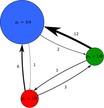
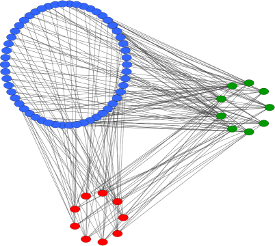
Figure 6. Schematic and realization of a random regular frame graph. A, the frame graph. The vertices of the frame (red = A, green = B, blue = C) are weighted according to their proportions $p$ in the random regular frame graph. The edge weights $D_{ij}$ set the between-class vertex degrees in the random regular frame graph. This frame will yield a random tripartite graph. B, realization of the graph on 72 vertices. In this instance, there are $1/8\times 72=9$ green and red vertices and $3/4\times 72=54$ blue vertices. Each blue vertex connects to $k_{CA}=1$ red vertex and $k_{CB}=2$ green vertices. This is actually a multigraph; with so few vertices, the probability that the configuration model algorithm yields parallel edges is high.

Sampling from $\mathcal{G}(n,H)$ can be performed similar to the configuration model, where each node is assigned as many half-edges as its degree, and these are wired together with a random matching (Newman (2010)). The detailed balance condition Eqn. (39) ensures that this matching is possible. Practically, we often have to generate many candidate matchings before the resulting graph is simple, but the probability of a simple graph is bounded away from zero for fixed $D$.

An example of a random regular frame graph is the bipartite, biregular random graph. The family $\mathcal{G}(n,m,d_{1},d_{2})$ is a random regular frame graph $\mathcal{G}(n+m,H)$, where the frame $H$ is the directed path on two vertices: $V=\{1,2\}$ and $E=\{(1,2),(2,1)\}$. The weights are taken as $p_{1}=n/(n+m)$, $p_{2}=m/(n+m)$, $D_{12}=d_{1}$, and $D_{21}=d_{2}$.

Another example random regular frame graph is shown in Figure 6. In this case, the frame $H$ has $V=\{A,B,C\}$ and $E=\{(A,B),(A,C),(B,A),(B,C),(C,A),(C,B)\}$ with weights $p$ and $D$ as shown in Figure 6A. We see that this generates a random tripartite graph with regular degrees between vertices in different independent sets, shown in Figure 6B.

6.2. Markov and related matrices of frame graphs

Now, we define a number of matrices associated with the frame and the sample of the random regular frame graph.

Let $G$ be a simple graph. Define $D_{G}=\mathrm{diag}(d_{G})$, the diagonal matrix of degrees in $G$. The Markov matrix $P=P(G)$ is defined as

$$P=D_{G}^{-1}A,$$

where $A=A(G)$ is the adjacency matrix. The Markov matrix is the row-normalized adjacency matrix, and it contains the transition probabilities of a random walker on the graph $G$. Let $L=I-\mathcal{L}=D_{G}^{-1/2}A\,D_{G}^{-1/2}$ be a matrix simply related to the normalized Laplacian. We call this the symmetrized Markov matrix. Then $P$ and $L$ have the same eigenvalues, but $L$ is symmetric, since $L_{ij}=\frac{A_{ij}}{\sqrt{d_{i}d_{j}}}$.

Suppose $G\sim\mathcal{G}(n,H)$, where the frame $H=(V,E,p,D)$. Another matrix that will be useful is what we call the Markov matrix of the frame $R$, where $R_{ij}=\frac{D_{ij}}{\sum_{j}D_{ij}}$. Thus, $R$ is a row-normalized $D$, in the same way that the Markov matrix $P$ is the row-normalized adjacency matrix $A$. Furthermore, $R$ is invariant under any uniform scaling of the degrees. Because of this equitable partition property of random regular frame graphs, eigenvectors of the frame matrices $D=D(H)$ or $R=R(H)$ lift to eigenvectors of $A=A(G)$ or $P=P(G)$, respectively. Suppose $Dx=\lambda x$, then it is a straightforward exercise to check that $A\tilde{x}=\lambda\tilde{x}$ for the piecewise constant vector

$$\tilde{x}=\left[\begin{array}[]{c}\mathbf{1}_{n_{1}}x_{1}\\ \mathbf{1}_{n_{2}}x_{2}\\ \vdots\end{array}\right].$$

Using the same procedure, we can lift any eigenpair of $R$ to an eigenpair of $P$ with the same eigenvalue.

6.2.1. Bounds on the eigenvalues of frame graphs in terms of blocks

The following result is due to Wan and Meilă (2015):

Proposition 18.

Let $G$ be a random regular frame graph $G(n,H)$, $P$ its Markov matrix, and $L$ the Laplacian with vertices ordered by class in both cases. Let $R$ be the Markov matrix of the frame $H=(V,E,p,D)$, with $|V(H)|=K$ classes. Define the matrices $L^{(kl)}$ as the $(k,l)$ block of $L$ with respect to the clustering of vertices by class. For $l\neq k$, let

$$M^{(kl)}=\left(\begin{array}[]{cc}0&L^{(kl)}\\ L^{(kl)}&0\end{array}\right)=\left(\begin{array}[]{cc}0&L^{(kl)}\\ L^{(lk)*}&0\end{array}\right).$$

For $l=k$, let $M^{(kk)}=L^{(kk)}$. Assume that all eigenvalues of $D$ are nonzero and pick a constant $C$ such that

$$\frac{|\lambda_{2}^{(kl)}|}{\lambda_{1}^{(kl)}}\leq C<1$$

for every $k,l=1,\ldots K$, where $\lambda_{1}^{(kl)}$ and $\lambda_{2}^{(kl)}$ are the leading and second eigenvalues of $M^{(kl)}$. Under these conditions, the eigenvalues of $P$ which are not eigenvalues of $R$ are bounded by

$$C\max_{k=1,\ldots,K}\left(R_{kk}+\sum_{l\neq k}\sqrt{R_{kl}R_{lk}}\right)\leq\frac{C}{2}\left(1+\max_{k=1,\ldots,K}\sum_{l=1}^{K}R_{lk}\right).$$

The spectrum of the Markov matrix $\sigma(P)$ enjoys a simple connection to $\sigma(A)$ when $A$ is the adjacency matrix of a graph drawn from $G(n,m,d_{1},d_{2})$. In this case, $L=\frac{A}{\sqrt{d_{1}d_{2}}}$, so the eigenvalues of $P$ are just the scaled eigenvalues of $A$. This and the spectral gap for bipartite, biregular random graphs, Theorem 4, lead to the following remark:

Remark.

For a random regular frame graph, $M^{(kl)}$ corresponds to the symmetrized Markov matrix $L$ of a bipartite biregular graph $G(n_{k},n_{l},D_{kl},D_{lk})$. Thus,

$$\frac{|\lambda_{2}^{(kl)}|}{\lambda_{1}^{(kl)}}\leq\frac{\sqrt{D_{kl}-1}+\sqrt{D_{lk}-1}}{\sqrt{D_{kl}D_{lk}}}+\epsilon.$$

Suppose we are given a frame that fits the conditions of Proposition 18; namely, $D$ cannot have any zero eigenvalues. Then we can uniformly grow the degrees, which leaves $R$ invariant, but allows us to reach an arbitrarily small $C$. This ensures that the leading $K$ eigenvalues of $P$ are equal to the eigenvalues of $R$. Note that this actually means that the entire random regular frame graph satifsfies a weak Ramanujan property. We now show that this guarantees spectral clustering.

6.3. Spectral clustering

Spectral clustering is a popular method of community detection. Because some eigenvectors of $P$, the Markov matrix of a random regular frame graph, are piecewise constant on classes, we can use them to recover the communities so long as those eigenvectors can be identified. Suppose there are $K$ total classes in our random regular frame graph. Then, given the eigenvectors $x^{1},x^{2},\ldots,x^{K}$, which are piecewise constant across classes, we can cluster vertices by class. For each vertex $v\in V(G)$, associate the vector $y^{v}\in\operatorname{\mathbb{R}}^{K}$ where $y^{v}_{j}=x^{j}_{v}$. Then if $y^{v}=y^{u}$ for $u,v\in V(G)$, vertices $u$ and $v$ belong to the same class. It is simple to recover these piecewise constant vectors $x^{1},x^{2},\ldots,x^{K}$ when they are the leading eigenvectors. These facts lead to the following theorem:

Theorem 19 (Spectral clustering guarantee in frame graphs).

Let $G$ be a random regular frame graph $G(n,H)$ and $P$ its Markov matrix. Let $R$ be the Markov matrix of the frame $H=(V,E,p,D)$, with $|V(H)|=K$ classes and $\lambda_{1}\geq\ldots\geq\lambda_{K}$ the eigenvalues of $R$ and $|\lambda_{K}|>0$. Then we can scale the degrees by some $\kappa\in\mathbb{N}$, $D\to\kappa D$, so that the vertex classes are recoverable by spectral clustering of the leading $K$ eigenvectors of $P$.

Remark.

The conditions of Theorem 19, while very general, are also weaker than may be expected using more sophisticated methods tailored to the specific frame model. We illustrate this with the following example.

6.3.1. Example: The regular stochastic block model

Brito, Dumitriu, Ganguly, Hoffman, and Tran (2016) and Barucca (2017) studied a regular stochastic block model, which can be seen as a special case of our frame model. Let the frame $H$ be the complete directed graph on two vertices, including self loops, where

$$D=\left(\begin{array}[]{cc}d_{1}&d_{2}\\ d_{2}&d_{1}\end{array}\right)$$

and $p=(1/2,1/2)$. Define the regular stochastic block model as $\mathcal{G}(2n,H)$. This is a graph with two classes of equal size, representing two communities of vertices, with within-class degree $d_{1}$ and between-class degree $d_{2}$. We assume $d_{1}>d_{2}$, since communities are more strongly connected within. Brito, Dumitriu, Ganguly, Hoffman, and Tran (2016) proved the following theorem:

Theorem 20.

If $(d_{1}-d_{2})^{2}>4(d_{1}+d_{2}-1)$, then there is an efficient algorithm for strong recovery, i.e. recovery of the exact communities with high probability as $n\to\infty$.

Theorem 20 gives a sharp bound on the degrees for recovery, which we can compare to our spectral clustering results. The eigenvalues of $D$ are $d_{1}+d_{2}$ and $d_{1}-d_{2}$, and the Markov matrix of the frame $R$ has eigenvalues $1$ and $(d_{1}-d_{2})/(d_{1}+d_{2})$. The diagonal blocks $L^{(11)}$ and $L^{(22)}$ each correspond to the Laplacian matrix of a $d_{1}$-regular random graph on $n$ vertices, whereas the off-diagonal block term $M^{(12)}$ corresponds to the Laplacian of a $d_{2}$-regular bipartite graph on $2n$ vertices. Using our results and the previously known results for regular random graphs (Friedman (2003, 2004); Bordenave, Lelarge, and Massoulié (2015)), we can pick some $C>2\sqrt{d_{2}-1}/d_{2}$ since $d_{1}>d_{2}$ and we will eventually take the degrees to be large. Using Proposition 18, we find that the spurious eigenvalues of $P$ come after the leading 2 eigenvalues if

$$\frac{2\sqrt{d_{2}-1}}{d_{2}}<\frac{d_{1}-d_{2}}{d_{1}+d_{2}},$$

to leading order in the degrees. Rearranging, we obtain the condition

$$(d_{1}-d_{2})^{2}>4(d_{2}-1)\left(\frac{d_{1}+d_{2}}{d_{2}}\right)^{2}.$$

Assuming $d_{2}/d_{1}=\beta<1$ fixed, and taking the limit $d_{1},d_{2}\to\infty$, we find that the result of Brito, Dumitriu, Ganguly, Hoffman, and Tran (2016) becomes

$$d_{1}>4\frac{1+\beta}{(1-\beta)^{2}}+o(1),$$

whereas our result becomes

$$d_{1}>\frac{4}{\beta}\left(\frac{1+\beta}{1-\beta}\right)^{2}+o(1),$$

illustrating that the spectral threshold is a factor of $(1+\beta)/\beta$ weaker.

7. Application: Low density parity check or expander codes

Another useful application of random graphs is as expanders, loosely defined as graphs where the neighborhood of a small set of nodes is large. Expander codes, also called low density parity check (LDPC) codes, were first introduced by Gallager in his PhD thesis (Gallager (1962)). These are a family of linear error correcting codes whose parity-check matrix is encoded in an expander graph. A linear code is a set $\mathcal{C}\subset\Sigma^{L}$, where a length $L$ codeword $x\in\mathcal{C}$ if and only if $Hx=0$. The alphabet $\Sigma$ is typically a finite field and $H\in\Sigma^{P\times L}$ is the parity check matrix. In the simplest case, $\Sigma=\mathbb{F}_{2}$ and each row of $H$ can be interpreted as a parity constraint on codewords. The performance of such codes depends on how good an expander that graph is, which in turn can be shown to depend on the separation of eigenvalues. For a good introduction and overview of the subject, see Richardson and Urbanke (2008).

Following Tanner (1981), we construct a code $\mathcal{C}$ from a $(d_{1},d_{2})$-regular bipartite graph $G$ on $n+m$ vertices and two smaller linear codes $\mathcal{C}_{1}$ and $\mathcal{C}_{2}$ of length $d_{1}$ and $d_{2}$, respectively. We write $\mathcal{C}_{1}=[d_{1},k_{1},\delta_{1}]$ and $\mathcal{C}_{2}=[d_{2},k_{2},\delta_{2}]$ with the usual convention of length, dimension, and minimum distance. We assume the codes are all binary, using the finite field $\mathbb{F}_{2}$ the codeword is $x\in\mathcal{C}\subset\mathbb{F}_{2}^{|E|}$ where $|E|=nd_{1}=md_{2}$. That is, we associate a bit to each edge in the graph bipartite graph $G$. Let $(e_{i}(v))_{i=1}^{d_{v}}$ represent the set of edges incident to a vertex $v$ in some arbitrary, fixed order. Then the vector $x\in\mathcal{C}$ if and only if the vectors $(x_{e_{1}(u)},x_{e_{2}(u)},\ldots,x_{e_{d_{1}}(u)})^{T}\in\mathcal{C}_{1}$ for all $u\in V_{1}$ and $(x_{e_{1}(v)},x_{e_{2}(v)},\ldots,x_{e_{d_{2}}(v)})^{T}\in\mathcal{C}_{2}$ for all $v\in V_{2}$. The final code $\mathcal{C}$ is also linear. With this construction, the code $\mathcal{C}$ has rate at least $k_{1}/d_{1}+k_{2}/d_{2}-1$ (Tanner (1981)).

Furthermore, Janwa and Lal (2003) proved the following bound on the minimum distance of the resulting code:

Theorem 21.

Suppose $\delta_{1}\geq\delta_{2}>\eta/2$, where $\eta$ is the second largest eigenvalue of the adjacency matrix of $G$. Then the code $\mathcal{C}$ has minimum distance

$$\delta\geq\frac{n}{d_{2}}\left(\delta_{1}\delta_{2}-\frac{\eta}{2}(\delta_{1}+\delta_{2})\right).$$

Corollary 22.

Suppose the code $\mathcal{C}$ is constructed from a biregular, bipartite random graph $G\sim\mathcal{G}(n,m,d_{1},d_{2})$ and the conditions of Theorem 21 hold. Then the minimum distance of $\mathcal{C}$ satisfies

$$\delta\geq\frac{n}{d_{2}}\left(\delta_{1}\delta_{2}-\frac{\sqrt{d_{1}-1}+\sqrt{d_{2}-1}}{2}(\delta_{1}+\delta_{2})-\epsilon_{n}\right).$$

We see that these Tanner codes will have maximal distance for smallest $\eta$, and used our main result, Theorem 4, to obtain the explicit bound in Corollary 22. By growing the graph, the above shows a way to construct arbitrarily large codes whose minimum distance remains proportional to the code size $nd_{1}$. That is, the relative distance $\delta/(nd_{1})$ is bounded away from zero as $n\to\infty$. However, the above bound will only be useful if it yields a positive result, which depends on the codes $\mathcal{C}_{1}$ and $\mathcal{C}_{2}$ as well as the degrees.

Remark.

In general, the performance guarantees on LDPC codes that are obtainable from graph eigenvalues are weaker than those that come from other methods. Although our method does guarantee high distance for some high degree codes, analysis of specific decoding algorithms or a probabilistic expander analyses yield better bounds that work for lower degrees (Richardson and Urbanke (2008)).

7.1. Example: An unbalanced code based on a $(14,9)$-regular bipartite graph

We illustrate the applicability of our distance bound with an example. Let $\mathcal{C}_{1}=[14,8,7]$ and $\mathcal{C}_{2}=[9,4,6]$. These can be achieved by using a Reed-Salomon code on the common field $\mathbb{F}_{q}$ for any $q>14$ (Richardson and Urbanke (2008)). We take $q=2^{4}=16$ for inputs that are actually binary, and this means each edge in the graph actually contains 4 bits of information. Employing Corollary 22, the Tanner code $\mathcal{C}$ will have relative minimum distance $\delta/(nd_{1})\geq 0.0014$ and rate at least $0.016$. Taking $n=216$ and $m=336$ gives the code a minimum distance of at least 4.

8. Application: Matrix completion

Assume we have some matrix $Y\in\operatorname{\mathbb{R}}^{n\times m}$ which has low “complexity.” Perhaps it is low-rank or simple by some other measure. If we observe $Y_{ij}$ for a limited set of entries $(i,j)\in E\subset[n]\times[m]$, then matrix completion is any method which constructs a matrix $\hat{Y}$ so that $\|\hat{Y}-Y\|$ is small, or even zero. Matrix completion has attracted significant attention in recent years as a tractable algorithm for making recommendations to users of online systems based on the tastes of other users (a.k.a. the Netflix problem). We can think of it as the matrix version of compressed sensing (Candès and Tao (2010); Candes and Plan (2010)).

Recently, a number of authors have studied the performance of matrix completion algorithms where the index set $E$ is the edge set of a regular random graph (Heiman, Schechtman, and Shraibman (2014); Bhojanapalli and Jain (2014); Gamarnik, Li, and Zhang (2017)). Heiman, Schechtman, and Shraibman (2014) describe a deterministic method of matrix completion, where they can give performance guarantees for a fixed observation set $E$ over many input matrices $Y$. The error of their reconstruction depends on the spectral gap of the graph. We expand upon the result of Heiman, Schechtman, and Shraibman (2014), extending it to rectangular matrix and improving their bounds in the process.

8.1. Matrix norms as measures of complexity and their relationships

We will employ a number of different matrix and vector norms in this Section. These are all related by the properties of the underlying Banach spaces. The complexity of $Y$ is measured using a factorization norm (also called the max-norm):

$$\gamma_{2}(Y)=\min_{UV^{*}=Y}\|U\|_{\ell_{2}\to\ell_{\infty}^{n}}\|V\|_{\ell_{2}\to\ell_{\infty}^{m}}.$$

The minimum is taken over all possible factorizations of $Y=UV^{*}$, and the norm $\|X\|_{\ell_{2}\to\ell_{\infty}^{n}}=\max_{i}\sqrt{\sum_{j}X^{2}_{ij}}$ returns the largest $\ell_{2}$ norm of a row. So, equivalently,

$$\gamma_{2}(Y)=\min_{UV^{*}=Y}\max_{i,j}\|u_{i}\|_{2}\,\|v_{j}\|_{2},$$

where $u_{i}$ and $v_{i}$ are the rows of $U$ and $V$. See Linial, Mendelson, Schechtman, and Shraibman (2007) for a number of results about the norm $\gamma_{2}$. In particular, note that

(40) $$\gamma_{2}(A\circ B)\leq\gamma_{2}(A)\gamma_{2}(B)$$

(41) $$\frac{1}{\sqrt{nm}}\|Y\|_{\rm Tr}\leq\gamma_{2}(Y)$$

(42) $$\gamma_{2}(Y)\leq\sqrt{\mathrm{rank}(Y)}\|Y\|_{\infty}.$$

Property (40) says that $\gamma_{2}$ is sub-multiplicative under the Hadamard product (Lee, Shraibman, and Špalek, 2008; Heiman, Schechtman, and Shraibman, 2014) and will be used in our proof. Properties (41) and (42) relate $\gamma_{2}$ to two common complexity measures of matrices, the trace norm (sum of singular values, i.e. the $\ell^{m}_{2}\to\ell^{n}_{2}$ nuclear norm) and rank. Note also the well-known fact that

$$\|Y\|_{\rm Tr}=\min_{UV^{*}=Y}\|U\|_{F}\|V\|_{F},$$

where $\|X\|_{F}=\sqrt{\sum_{ij}X_{ij}^{2}}$ is the Frobenius norm. We see that the trace norm constrains factors $U$ and $V$ to be small on average via $\|\cdot\|_{F}$, whereas the norm $\gamma_{2}$ is similar but constrains factors uniformly via $\|\cdot\|_{\ell_{2}\to\ell_{\infty}^{n}}$. However, we should note that computing $\gamma_{2}(Y)$ is more costly than the trace norm, which can be performed with just the singular value decomposition, although still possible in polynomial time with convex programming (Heiman, Schechtman, and Shraibman, 2014).

8.2. Matrix completion generalization bounds

The method of matrix completion that we study is to return the matrix $X$ which is the solution to:

(43) $$\underset{X}{\text{minimize}} \gamma_{2}(X)$$

subject to $$X_{ij}=Y_{ij},\;(i,j)\in E.$$

The $\gamma_{2}$ norm was first proposed by Srebro and Shraibman (2005); Srebro, Rennie, and Jaakkola (2005) as a robust complexity measure, and it was shown to be an effective and practical regularization on real datasets (Lee, Recht, Srebro, Tropp, and Salakhutdinov, 2010; Recht and Ré, 2013).

Heiman, Schechtman, and Shraibman (2014) analyze the performance of the convex program (43) for a square matrix $Y$ using an expander argument, assuming that $E$ is the edge set of a $d$-regular graph with second eigenvalue $\eta$. They obtain the following theorem:

Theorem 23 (Heiman, Schechtman, and Shraibman (2014)).

Let $E$ be the set of edges of a $d$-regular graph with second eigenvalue bound $\eta$. For every $Y\in\operatorname{\mathbb{R}}^{n\times n}$, if $\hat{Y}$ is the output of the optimization problem (43), then

$$\frac{1}{n^{2}}\|\hat{Y}-Y\|_{F}^{2}\leq c\gamma_{2}(Y)^{2}\frac{\eta}{d},$$

where $c=8K_{G}\leq 14.3$ is a universal constant and $\|\cdot\|_{F}$ is the Frobenius norm.

Considering sampling following the biadjacency matrix of a bipartite graph, we find a similar result which also applies to rectangular matrices. If $n=m$ and $d_{1}=d_{2}=d$, our bound is equivalent to that of Theorem 23, but with constants improved by a factor of two due to stronger mixing in bipartite graphs. Intuitively, using a biadjacency matrix is a “more random” way of sampling than using an adjacency matrix, since it is not symmetric.

Theorem 24.

Let $E$ be the set of edges of a $(d_{1},d_{2})$-regular graph with second eigenvalue bound $\eta$. For every $Y\in\operatorname{\mathbb{R}}^{n\times m}$, if $\hat{Y}$ is the output of the optimization problem (43), then

$$\frac{1}{nm}\|\hat{Y}-Y\|_{F}^{2}\leq c\gamma_{2}(Y)^{2}\frac{\eta}{\sqrt{d_{1}d_{2}}},$$

where $c=4K_{G}\leq 7.13$.

Proof.

We start by considering a rank-1 sign matrix $S=uv^{*}$, where $u,v\in\{-1,1\}^{n\times m}$. Let $S^{\prime}=\frac{1}{2}(S+J)$, where $J$ is the all-ones matrix, so that $S^{\prime}$ has the entries of -1 in $S$ replaced by zeros. Then $S^{\prime}=1_{A}1_{B}^{*}+1_{A^{c}}1_{B^{c}}^{*}$ for subsets $A\subset V_{1}=[n]$ and $B\subset V_{2}=[m]$, where $A=\{i:u_{i}=1\}$ and $B=\{j:v_{j}=1\}$. Consider the expression

$$\left|\frac{1}{nm}\sum_{i,j}s_{ij}-\frac{1}{|E|}\sum_{(i,j)\in E}s_{ij}\right| =\left|\frac{1}{nm}\sum_{i,j}(2s^{\prime}_{ij}-1)-\frac{1}{|E|}\sum_{(i,j)\in E}(2s^{\prime}_{ij}-1)\right|$$

$$=2\left|\frac{1}{nm}\sum_{i,j}s^{\prime}_{ij}-\frac{1}{|E|}\sum_{(i,j)\in E}s^{\prime}_{ij}\right|$$

$$=2\left|\frac{|A||B|+|A^{c}||B^{c}|}{nm}-\frac{E(A,B)+E(A^{c},B^{c})}{|E|}\right|$$

$$\leq 2\left|\frac{|A||B|}{nm}-\frac{E(A,B)}{|E|}\right|+2\left|\frac{|A^{c}||B^{c}|}{nm}-\frac{E(A^{c},B^{c})}{|E|}\right|.$$

The following is a bipartite version of the expander mixing lemma (De Winter, Schillewaert, and Verstraete, 2012):

$$\left|\frac{E(A,B)}{|E|}-\frac{|A||B|}{nm}\right|\leq\frac{\eta}{\sqrt{d_{1}d_{2}}}\sqrt{\frac{|A||B|}{nm}\left(1-\frac{|A|}{n}\right)\left(1-\frac{|B|}{m}\right)}\\ =\frac{\eta}{\sqrt{d_{1}d_{2}}}\sqrt{\frac{|A||B||A^{c}||B^{c}|}{(nm)^{2}}}.$$

We find that

$$\left|\frac{1}{nm}\sum_{i,j}s_{ij}-\frac{1}{|E|}\sum_{(i,j)\in E}s_{ij}\right| \leq\frac{4\eta}{\sqrt{d_{1}d_{2}}}\sqrt{\frac{|A||B||A^{c}||B^{c}|}{(nm)^{2}}}$$

$$=\frac{4\eta}{\sqrt{d_{1}d_{2}}}\sqrt{xy(1-x)(1-y)}$$

$$\leq\frac{\eta}{\sqrt{d_{1}d_{2}}},$$

since $xy(1-x)(1-y)$ attains a maximal value of $2^{-4}$ for $0\leq x,y\leq 1$.

The rest of the proof develops identical to the results of Heiman, Schechtman, and Shraibman (2014), which we include for completeness. We apply the result for rank-1 sign matrices to any matrix $R$. Let $R=\sum_{i}\alpha_{i}S^{i}$, where $S^{i}$ is a rank-1 sign matrix and $\alpha_{i}\in\operatorname{\mathbb{R}}$. For a general matrix $R$, this might require many rank-1 sign matrices. Define the sign nuclear norm $\nu(R)=\sum_{i}|\alpha_{i}|$. Then,

$$\left|\frac{1}{nm}\sum_{i,j}r_{ij}-\frac{1}{|E|}\sum_{(i,j)\in E}r_{ij}\right|\leq\nu(R)\frac{\eta}{\sqrt{d_{1}d_{2}}}.$$

It is a consequence of Grothendieck’s inequality, a well-known theorem in functional analysis, that there exists a universal constant $1.5\leq K_{G}\leq 1.8$ so that $\gamma_{2}(X)\leq\nu(X)\leq K_{G}\gamma_{2}(X)$ for any real matrix $X$; see Heiman, Schechtman, and Shraibman (2014).

Now, let the matrix of residuals $R=(\hat{Y}-Y)\circ(\hat{Y}-Y)$, where $\circ$ is the Hadamard entry-wise product of two matrices, so that $R_{ij}=(\hat{Y}_{ij}-Y_{ij})^{2}$. Since

$$\frac{1}{|E|}\sum_{(i,j)\in E}r_{ij}=0,$$

we conclude that

$$\frac{1}{nm}\sum_{i,j}r_{ij}\leq\nu(R)\frac{\eta}{\sqrt{d_{1}d_{2}}}\leq K_{G}\gamma_{2}(R)\frac{\eta}{\sqrt{d_{1}d_{2}}}.$$

Furthermore, $\gamma_{2}(R)\leq\gamma_{2}(\hat{Y}-Y)^{2}\leq(\gamma_{2}(\hat{Y})+\gamma_{2}(Y))^{2}$ by (40) and the triangle inequality. Since $\hat{Y}$ is the output of the algorithm and $Y$ is a feasible solution, $\gamma_{2}(\hat{Y})\leq\gamma_{2}(Y)$. Thus, $\gamma_{2}(R)\leq 4\gamma_{2}(Y)^{2}$ and the proof is finished. ∎

8.3. Noisy matrix completion bounds

Furthermore, our analysis easily extends to the case where the matrix we observe is corrupted with noise. As mentioned in the above remark, similar results will hold for the trace norm. In the noisy case, we solve the problem

(44) $$\underset{X}{\text{minimize}} \gamma_{2}(X)$$

subject to $$\frac{1}{|E|}\sum_{(i,j)\in E}(X_{ij}-Z_{ij})^{2}\leq\delta^{2}$$

and obtain the following theorem:

Theorem 25.

Suppose we observe $Z_{ij}=Y_{ij}+\epsilon_{ij}$ with bounded error

$$\frac{1}{|E|}\sum_{(i,j)\in E}\epsilon_{ij}^{2}\leq\delta^{2}.$$

Then solving the optimization problem (44) will yield a bound of

$$\frac{1}{nm}\|\hat{Y}-Y\|_{F}^{2}\leq c\gamma_{2}(Y)^{2}\frac{\eta}{\sqrt{d_{1}d_{2}}}+4\delta^{2},$$

where $c=4K_{G}\leq 7.13$.

Proof.

Denote $\hat{Y}$ the solution to P44. It will be useful to introduce the sampling operator $\mathcal{P}_{E}:\operatorname{\mathbb{R}}^{n\times m}\to\operatorname{\mathbb{R}}^{n\times m}$, where $(\mathcal{P}_{E}(X))_{ij}=X_{ij}$ if $(i,j)\in E$ and 0 otherwise. Again let $R=(\hat{Y}-Y)\circ(\hat{Y}-Y)$ be the matrix of squared errors, then

$$\left|\frac{1}{nm}\|\hat{Y}-Y\|_{F}^{2}-\frac{1}{|E|}\|\mathcal{P}_{E}(\hat{Y}-Y)\|_{F}^{2}\right| =\left|\frac{1}{nm}\sum_{i,j}(\hat{Y}_{ij}-Y_{ij})^{2}-\frac{1}{|E|}\sum_{(i,j)\in E}(\hat{Y}_{ij}-Y_{ij})^{2}\right|$$

$$\leq K_{G}\gamma_{2}(R)\frac{\eta}{\sqrt{d_{1}d_{2}}}.$$

However, since $Y$ is a feasible solution to P44, we have

$$\gamma_{2}(\hat{Y})\leq\gamma_{2}(Y).$$

Applying (40) and the triangle inequality,

$$\gamma_{2}(R)\leq\left(\gamma_{2}(\hat{Y}-Y)\right)^{2}\leq\left(\gamma_{2}(\hat{Y})+\gamma_{2}(Y)\right)^{2}\leq 4\gamma_{2}(Y)^{2}.$$

Using the triangle inequality again gives

$$\|\mathcal{P}_{E}(\hat{Y}-Y)\|_{F}\leq\|\mathcal{P}_{E}(\hat{Y}-Z)\|_{F}+\|\mathcal{P}_{E}(Z-Y)\|_{F}\leq 2\delta\sqrt{|E|},$$

taking into account the bound on the observation errors. Because

$$\frac{1}{nm}\|\hat{Y}-Y\|_{F}^{2}\leq\left|\frac{1}{nm}\|\hat{Y}-Y\|_{F}^{2}-\frac{1}{|E|}\|\mathcal{P}_{E}(\hat{Y}-Y)\|_{F}^{2}\right|+\frac{1}{|E|}\|\mathcal{P}_{E}(\hat{Y}-Y)\|_{F}^{2}$$

we get the final bound

$$\frac{1}{nm}\|\hat{Y}-Y\|_{F}^{2}\leq 4K_{G}\gamma_{2}(Y)^{2}\frac{\eta}{\sqrt{d_{1}d_{2}}}+4\delta^{2}.$$

∎

8.4. Application of the spectral gap

Theorem 24 provides a bound on the mean squared error of the approximation $X$. Directly applying Theorem 4, we obtain the following bound on the generalization error of the algorithm using a random biregular, bipartite graph:

Corollary 26.

Let $E$ be sampled from a $\mathcal{G}(n,m,d_{1},d_{2})$ random graph. For every $Y\in\operatorname{\mathbb{R}}^{n\times m}$, if $\hat{Y}$ is the output of the optimization problem (43), then

$$\frac{1}{nm}\|\hat{Y}-Y\|_{F}^{2}\leq c\gamma_{2}(Y)^{2}\frac{\sqrt{d_{1}-1}+\sqrt{d_{2}-1}+\epsilon_{n}}{\sqrt{d_{1}d_{2}}},$$

where $c=4K_{G}\leq 7.13$ is a universal constant.

Appendix A List of symbols

$A$	adjacency matrix
$B$	non-backtracking matrix
$X^{*}$	transpose of the matrix $X$
$\sigma(X)$	the eigenvalue spectrum of a matrix $X$
$\eta$	second-largest eigenvalue of the adjacency matrix $A$
$\lambda_{i}(X)$	the $i$th largest eigenvalue, in absolute value, of a matrix $X$
$\mathcal{G}(n,m,d_{1},d_{2})$	family of bipartite $d_{1},d_{2}$-regular random graphs on $n,m$ vertices
$d$	the maximum degree: $d=\max\{d_{1},d_{2}\}=d_{1}$ without loss of generality
$V(G)$	vertex set of graph or subgraph $G$
$E(G)$	edge set of a graph or subgraph $G$
$\vec{E}(G)$	oriented edge set of a graph or subgraph $G$
$\chi$	tree excess of a graph or subgraph $G$: $\chi(G)=|V(G)|-|E(G)|+1$
$\gamma$	a path
$\Gamma_{ef}^{\ell}$	non-backtracking paths of length $\ell+1$ from oriented edge $e$ to $f$
$F_{ef}^{\ell}$	non-backtracking, tangle-free paths of length $\ell+1$ from oriented edge $e$ to $f$
$T_{ef}^{\ell,j}$	non-backtracking paths of length $\ell+1$, from $e$ to $f$, such that the overall path is tangled but the first $j$ and last $\ell-j$ form tangle-free subpaths
$\|\cdot\|$	$\ell^{2}$-norm of a vector or spectral norm of a matrix
$\|\cdot\|_{F}$	Frobenius norm of a matrix

References

- Alon [1986] Noga Alon. Eigenvalues and expanders. Combinatorica, 6(2):83–96, June 1986. ISSN 0209-9683, 1439-6912. doi: 10.1007/BF02579166.
- Angel et al. [2007] Omer Angel, Joel Friedman, and Shlomo Hoory. The Non-Backtracking Spectrum of the Universal Cover of a Graph. arXiv:0712.0192 [math], December 2007.
- Angel et al. [2015] Omer Angel, Joel Friedman, and Shlomo Hoory. The non-backtracking spectrum of the universal cover of a graph. Transactions of the American Mathematical Society, 367(6):4287–4318, 2015. ISSN 0002-9947, 1088-6850. doi: 10.1090/S0002-9947-2014-06255-7.
- Barrett et al. [2017] Wayne Barrett, Amanda Francis, and Benjamin Webb. Equitable decompositions of graphs with symmetries. Linear Algebra and its Applications, 513(Supplement C):409–434, January 2017. ISSN 0024-3795. doi: 10.1016/j.laa.2016.10.017.
- Barucca [2017] Paolo Barucca. Spectral partitioning in equitable graphs. Physical Review E, 95(6):062310, June 2017. doi: 10.1103/PhysRevE.95.062310.
- Bass [1992] Hyman Bass. The Ihara-Selberg zeta function of a tree lattice. International Journal of Mathematics, 03(06):717–797, December 1992. ISSN 0129-167X. doi: 10.1142/S0129167X92000357.
- Bender [1974] Edward A. Bender. The asymptotic number of non-negative integer matrices with given row and column sums. Discrete Mathematics, 10(2):217–223, January 1974. ISSN 0012-365X. doi: 10.1016/0012-365X(74)90118-6.
- Bender and Canfield [1978] Edward A Bender and E. Rodney Canfield. The asymptotic number of labeled graphs with given degree sequences. Journal of Combinatorial Theory, Series A, 24(3):296–307, May 1978. ISSN 0097-3165. doi: 10.1016/0097-3165(78)90059-6.
- Bhojanapalli and Jain [2014] Srinadh Bhojanapalli and Prateek Jain. Universal Matrix Completion. In PMLR, pages 1881–1889, January 2014.
- Bollobás [1980] Béla Bollobás. A Probabilistic Proof of an Asymptotic Formula for the Number of Labelled Regular Graphs. European Journal of Combinatorics, 1(4):311–316, December 1980. ISSN 0195-6698. doi: 10.1016/S0195-6698(80)80030-8.
- Bollobás [2001] Béla Bollobás. Random Graphs. Cambridge University Press, Cambridge, 2001. ISBN 978-0-511-81406-8.
- Bordenave [2015] Charles Bordenave. A new proof of Friedman’s second eigenvalue Theorem and its extension to random lifts. arXiv:1502.04482 [math], February 2015.
- Bordenave and Lelarge [2010] Charles Bordenave and Marc Lelarge. Resolvent of large random graphs. Random Structures & Algorithms, 37(3):332–352, October 2010. ISSN 10429832. doi: 10.1002/rsa.20313.
- Bordenave et al. [2015] Charles Bordenave, Marc Lelarge, and Laurent Massoulié. Non-backtracking spectrum of random graphs: Community detection and non-regular Ramanujan graphs. arXiv:1501.06087 [cs, math], January 2015.
- Brito et al. [2015] Gerandy Brito, Ioana Dumitriu, Shirshendu Ganguly, Christopher Hoffman, and Linh V. Tran. Recovery and Rigidity in a Regular Stochastic Block Model. arXiv:1507.00930 [math], July 2015.
- Brito et al. [2016] Gerandy Brito, Ioana Dumitriu, Shirshendu Ganguly, Christopher Hoffman, and Linh V. Tran. Recovery and Rigidity in a Regular Stochastic Block Model. In Proceedings of the Twenty-Seventh Annual ACM-SIAM Symposium on Discrete Algorithms, SODA, pages 1589–1601, Philadelphia, PA, USA, 2016. Society for Industrial and Applied Mathematics. ISBN 978-1-61197-433-1.
- Candes and Plan [2010] E. J. Candes and Y. Plan. Matrix Completion With Noise. Proceedings of the IEEE, 98(6):925–936, June 2010. ISSN 0018-9219. doi: 10.1109/JPROC.2009.2035722.
- Candès and Tao [2010] E.J. Candès and T. Tao. The Power of Convex Relaxation: Near-Optimal Matrix Completion. IEEE Transactions on Information Theory, 56(5):2053–2080, May 2010. ISSN 0018-9448. doi: 10.1109/TIT.2010.2044061.
- Cook [2017] Nicholas A. Cook. On the singularity of adjacency matrices for random regular digraphs. Probability Theory and Related Fields, 167(1-2):143–200, February 2017. ISSN 0178-8051, 1432-2064. doi: 10.1007/s00440-015-0679-8.
- Coste [2017] Simon Coste. The Spectral Gap of Sparse Random Digraphs. arXiv:1708.00530 [math], August 2017.
- Costello and Vu [2008] Kevin P. Costello and Van H. Vu. The rank of random graphs. Random Structures & Algorithms, 33(3):269–285, October 2008. ISSN 1098-2418. doi: 10.1002/rsa.20219.
- De Winter et al. [2012] Stefaan De Winter, Jeroen Schillewaert, and Jacques Verstraete. Large Incidence-free Sets in Geometries. The Electronic Journal of Combinatorics, 19(4):P24, November 2012. ISSN 1077-8926.
- Deshpande et al. [2018] Yash Deshpande, Andrea Montanari, Ryan O’Donnell, Tselil Schramm, and Subhabrata Sen. The threshold for SDP-refutation of random regular NAE-3SAT. arXiv:1804.05230 [cs, math], April 2018.
- Dumitriu and Johnson [2016] Ioana Dumitriu and Tobias Johnson. The Marčenko-Pastur law for sparse random bipartite biregular graphs. Random Structures & Algorithms, 48(2):313–340, March 2016. ISSN 1098-2418. doi: 10.1002/rsa.20581.
- Feng and Li [1996] Keqin Feng and Wen-Ch’ing Winnie Li. Spectra of Hypergraphs and Applications. Journal of Number Theory, 60(1):1–22, September 1996. ISSN 0022-314X. doi: 10.1006/jnth.1996.0109.
- Fortunato [2010] Santo Fortunato. Community detection in graphs. Physics Reports, 486(3–5):75–174, February 2010. ISSN 0370-1573. doi: 10.1016/j.physrep.2009.11.002.
- Friedman [2003] Joel Friedman. Relative expanders or weakly relatively Ramanujan graphs. Duke Mathematical Journal, 118(1):19–35, May 2003. ISSN 0012-7094, 1547-7398. doi: 10.1215/S0012-7094-03-11812-8.
- Friedman [2004] Joel Friedman. A proof of Alon’s second eigenvalue conjecture and related problems. arXiv:cs/0405020, May 2004.
- Friedman and Kohler [2014] Joel Friedman and David-Emmanuel Kohler. The Relativized Second Eigenvalue Conjecture of Alon. arXiv:1403.3462 [cs, math], March 2014.
- Gallager [1962] R. Gallager. Low-density parity-check codes. IRE Transactions on Information Theory, 8(1):21–28, January 1962. ISSN 0096-1000. doi: 10.1109/TIT.1962.1057683.
- Gamarnik et al. [2017] David Gamarnik, Quan Li, and Hongyi Zhang. Matrix Completion from $O(n)$ Samples in Linear Time. arXiv:1702.02267 [cs, math, stat], February 2017.
- Godsil and Mohar [1988] C. D. Godsil and B. Mohar. Walk generating functions and spectral measures of infinite graphs. Linear Algebra and its Applications, 107(Supplement C):191–206, August 1988. ISSN 0024-3795. doi: 10.1016/0024-3795(88)90245-5.
- Heiman et al. [2014] Eyal Heiman, Gideon Schechtman, and Adi Shraibman. Deterministic algorithms for matrix completion. Random Structures & Algorithms, 45(2):306–317, September 2014. ISSN 1098-2418. doi: 10.1002/rsa.20483.
- Holland et al. [1983] Paul W. Holland, Kathryn Blackmond Laskey, and Samuel Leinhardt. Stochastic blockmodels: First steps. Social Networks, 5(2):109–137, June 1983. ISSN 0378-8733. doi: 10.1016/0378-8733(83)90021-7.
- Hoory et al. [2006] Shlomo Hoory, Nathan Linial, and Avi Wigderson. Expander graphs and their applications. Bulletin of the American Mathematical Society, 43(4):439–561, 2006. ISSN 0273-0979, 1088-9485. doi: 10.1090/S0273-0979-06-01126-8.
- Huang [2018a] Jiaoyang Huang. Invertibility of adjacency matrices for random -regular graphs. arXiv preprint arXiv:1807.06465, 2018a.
- Huang [2018b] Jiaoyang Huang. Invertibility of adjacency matrices for random -regular directed graphs. arXiv preprint arXiv:1806.01382, 2018b.
- Janwa and Lal [2003] H. Janwa and A. K. Lal. On Tanner Codes: Minimum Distance and Decoding. Applicable Algebra in Engineering, Communication and Computing, 13(5):335–347, February 2003. ISSN 0938-1279, 1432-0622. doi: 10.1007/s00200-003-0098-4.
- Kempton [2016] Mark Kempton. Non-Backtracking Random Walks and a Weighted Ihara’s Theorem. Open Journal of Discrete Mathematics, 06(04):207–226, 2016. ISSN 2161-7635, 2161-7643. doi: 10.4236/ojdm.2016.64018.
- Kotani and Sunada [2000] Motoko Kotani and Toshikazu Sunada. Zeta Functions of Finite Graphs. Journal of mathematical sciences, the University of Tokyo, 7(1):7–25, 2000. ISSN 13405705.
- Lee et al. [2010] Jason D Lee, Ben Recht, Nathan Srebro, Joel Tropp, and Russ R Salakhutdinov. Practical Large-Scale Optimization for Max-norm Regularization. In J. Lafferty, C. Williams, J. Shawe-Taylor, R. Zemel, and A. Culotta, editors, Advances in Neural Information Processing Systems, volume 23, pages 1297–1305. Curran Associates, Inc., 2010.
- Lee et al. [2008] Troy Lee, Adi Shraibman, and Robert Špalek. A Direct Product Theorem for Discrepancy. In 2008 23rd Annual IEEE Conference on Computational Complexity, pages 71–80, June 2008. doi: 10.1109/CCC.2008.25.
- Li and Solé [1996] Wen-Ch’ing Winnie Li and Patrick Solé. Spectra of Regular Graphs and Hypergraphs and Orthogonal Polynomials. European Journal of Combinatorics, 17(5):461–477, July 1996. ISSN 0195-6698. doi: 10.1006/eujc.1996.0040.
- Linial et al. [2007] Nati Linial, Shahar Mendelson, Gideon Schechtman, and Adi Shraibman. Complexity measures of sign matrices. Combinatorica, 27(4):439–463, July 2007. ISSN 0209-9683, 1439-6912. doi: 10.1007/s00493-007-2160-5.
- Litvak et al. [2016] Alexander E. Litvak, Anna Lytova, Konstantin Tikhomirov, Nicole Tomczak-Jaegermann, and Pierre Youssef. Anti-concentration property for random digraphs and invertibility of their adjacency matrices. Comptes Rendus Mathematique, 354(2):121–124, February 2016. ISSN 1631-073X. doi: 10.1016/j.crma.2015.12.002.
- Litvak et al. [2017] Alexander E. Litvak, Anna Lytova, Konstantin Tikhomirov, Nicole Tomczak-Jaegermann, and Pierre Youssef. Adjacency matrices of random digraphs: Singularity and anti-concentration. Journal of Mathematical Analysis and Applications, 445(2):1447–1491, January 2017. ISSN 0022-247X. doi: 10.1016/j.jmaa.2016.08.020.
- Lubetzky and Sly [2010] Eyal Lubetzky and Allan Sly. Cutoff phenomena for random walks on random regular graphs. Duke Mathematical Journal, 153(3):475–510, June 2010. ISSN 0012-7094, 1547-7398. doi: 10.1215/00127094-2010-029.
- Marcus et al. [2013a] A. Marcus, D. A. Spielman, and N. Srivastava. Interlacing Families I: Bipartite Ramanujan Graphs of All Degrees. In 2013 IEEE 54th Annual Symposium on Foundations of Computer Science, pages 529–537, October 2013a. doi: 10.1109/FOCS.2013.63.
- Marcus et al. [2013b] Adam Marcus, Daniel A. Spielman, and Nikhil Srivastava. Interlacing Families II: Mixed Characteristic Polynomials and the Kadison-Singer Problem. arXiv:1306.3969 [math], June 2013b.
- Massoulie [2013] Laurent Massoulie. Community detection thresholds and the weak Ramanujan property. arXiv:1311.3085 [cs], November 2013.
- McKay [1981] Brendan D McKay. Subgraphs of random graphs with specified degrees. Congressus Numerantium, 33:213–223, 1981.
- McKay [1984] Brendan D McKay. Asymptotics for 0-1 Matrices with Prescribed Line Sums. Enumeration and Design, pages 225–238, 1984.
- Mizuno and Sato [2003] Hirobumi Mizuno and Iwao Sato. The semicircle law for semiregular bipartite graphs. Journal of Combinatorial Theory, Series A, 101(2):174–190, February 2003. ISSN 0097-3165. doi: 10.1016/S0097-3165(02)00010-9.
- Newman and Martin [2014] M. E. J. Newman and Travis Martin. Equitable random graphs. Physical Review E, 90(5):052824, November 2014. doi: 10.1103/PhysRevE.90.052824.
- Newman [2010] Mark Newman. Networks: An Introduction. Oxford University Press, March 2010. ISBN 978-0-19-150070-1.
- Recht and Ré [2013] Benjamin Recht and Christopher Ré. Parallel stochastic gradient algorithms for large-scale matrix completion. Mathematical Programming Computation, 5(2):201–226, June 2013. ISSN 1867-2957. doi: 10.1007/s12532-013-0053-8.
- Richardson and Urbanke [2003] T. Richardson and R. Urbanke. The renaissance of Gallager’s low-density parity-check codes. IEEE Communications Magazine, 41(8):126–131, August 2003. ISSN 0163-6804. doi: 10.1109/MCOM.2003.1222728.
- Richardson and Urbanke [2008] Tom Richardson and Ruediger Urbanke. Modern Coding Theory. Cambridge University Press, New York, NY, USA, 2008. ISBN 978-0-521-85229-6.
- Srebro and Shraibman [2005] Nathan Srebro and Adi Shraibman. Rank, Trace-Norm and Max-Norm. In Learning Theory, Lecture Notes in Computer Science, pages 545–560. Springer, Berlin, Heidelberg, June 2005. ISBN 978-3-540-26556-6 978-3-540-31892-7. doi: 10.1007/11503415˙37.
- Srebro et al. [2005] Nathan Srebro, Jason Rennie, and Tommi S. Jaakkola. Maximum-Margin Matrix Factorization. In L. K. Saul, Y. Weiss, and L. Bottou, editors, Advances in Neural Information Processing Systems 17, pages 1329–1336. MIT Press, 2005.
- Tanner [1981] R. Tanner. A recursive approach to low complexity codes. IEEE Transactions on Information Theory, 27(5):533–547, September 1981. ISSN 0018-9448. doi: 10.1109/TIT.1981.1056404.
- Wan and Meilă [2015] Yali Wan and Marina Meilă. A class of network models recoverable by spectral clustering. In C. Cortes, N. D. Lawrence, D. D. Lee, M. Sugiyama, and R. Garnett, editors, Advances in Neural Information Processing Systems 28, pages 3285–3293. Curran Associates, Inc., 2015.
- Watanabe and Fukumizu [2009] Yusuke Watanabe and Kenji Fukumizu. Graph zeta function in the bethe free energy and loopy belief propagation. Advances in Neural Information Processing Systems, 2009.
- Wormald [1981] Nicholas C. Wormald. The asymptotic connectivity of labelled regular graphs. Journal of Combinatorial Theory, Series B, 31(2):156–167, October 1981. ISSN 0095-8956. doi: 10.1016/S0095-8956(81)80021-4.