Converse bounds for quantum and private
communication over Holevo-Werner channels

Abstract

Werner states have a host of interesting properties, which often serve to illuminate the unusual properties of quantum information. Starting from these states, one may define a family of quantum channels, known as the Holevo-Werner channels, which themselves afford several unusual properties. In this paper we use the teleportation covariance of these channels to upper bound their two-way assisted quantum and secret-key capacities. This bound may be expressed in terms of relative entropy distances, such as the relative entropy of entanglement, and also in terms of the squashed entanglement. Most interestingly, we show that the relative entropy bounds are strictly subadditive for a sub-class of the Holevo-Werner channels, so that their regularisation provides a tighter performance. These information-theoretic results are first found for point-to-point communication and then extended to repeater chains and quantum networks, under different types of routing strategies.

I Introduction

The area of quantum information and computation NielsenChuang ; Hayashi ; HolevoBOOK ; RMP ; HayashiINTRO is one of the fastest growing fields. Understanding how quantum information is transmitted is necessary not only for the development of a future quantum Internet Kimble2008 ; HybridINTERNET ; ref1 ; ref3 ; ref4 ; ref5 ; ref6 ; Meter but also for the construction of practical quantum key distribution (QKD) crypt1 ; crypt2 ; crypt3 ; crypt4 networks. Motived by this, there is much interest in trying to establish the optimal performance in the transmission of quantum bits (qubits), entanglement bits (ebits) and secret bits between two remote users. This is a theoretical framework which is a direct quantum generalization of Shannon’s theory of information Shannon ; Cover&Thomas . In the quantum setting, there are different types of maximum rates, i.e., capacities, that may be defined for a given quantum channel. These include the classical capacity (transmission of classical bits), the entanglement distribution capacity (distribution of ebits), the quantum capacity (transmission of qubits), the private capacity (transmission of private bits), and the secret-key capacity (distribution of secret bits). All these capacities may be defined allowing side local operations (LOs) and classical communication (CC) either one-way or two-way between the remote parties.

We shall focus on the use of LOs assisted by two-way CC, also known as “adaptive LOCCs”. The maximization over these types of LOCCs leads to the definition of corresponding two-way assisted capacities. In particular, in this work we are interested in the two-way quantum capacity $Q_{2}$ (which is equal to the two-way entanglement distribution capacity $D_{2}$) and the secret-key capacity $K$ (which is equal to the two-way private capacity $P_{2}$). Generally, these capacities are extremely difficult to calculate because they involve quantum protocols based on adaptive LOCCs, where input states and the output measurements are optimized in an interactive way by the two remote parties. Similar adaptive protocols may be considered in other tasks, such as quantum hypothesis testing Harrow ; PirCo ; PBT and quantum metrology PirCo ; Rafal ; ReviewMETRO ; adaptive2 ; ada3 ; ada4 ; ada5 ; HWmetro .

Building on a number of preliminary tools B2main ; Gatearray ; SamBrassard ; HoroTEL ; Gottesman ; SougatoBowen ; Knill ; WernerTELE ; Cirac ; Aliferis ; Niset ; MHthesis ; Wolfnotes ; Leung and generalizing ideas therein to arbitrary dimension and arbitrary tasks, Ref. Stretching showed how to use the LOCC simulation NoteLOCC of a quantum channel to reduce an arbitrary adaptive protocol into a simpler block version. More precisely, Ref. Stretching showed how the suitable combination of an adaptive-to-block reduction (teleportation stretching) with an entanglement measure, such as the relative entropy of entanglement (REE) RMPrelent ; VedFORMm ; Pleniom , allows one to reduce the expression of $Q_{2}$ and $K$ to a computable single-letter version. In this way, Ref. Stretching established the two-way capacities of several quantum channels, including the bosonic lossy channel RMP , the quantum-limited amplifier, the dephasing and the erasure channel NielsenChuang . The secret-key capacity of the erasure channel was also established in a simultaneous work GEW by using a different approach based on the squashed entanglement squash , which also appears to be powerful in the case of the amplitude damping channel GEW ; Stretching . Note that, prior to these results, only the $Q_{2}$ of the erasure channel was known ErasureChannelm .

One of the golden rules to apply the previous techniques is teleportation covariance, first considered for discrete variable (DV) channels MHthesis ; Wolfnotes ; Leung and then extended to any dimension, finite or infinite Stretching . This is the property of a quantum channel to “commute” with the random unitaries of quantum teleportation tele ; teleCV ; telereview ; teleCV2 . Because the Holevo-Werner (HW) channels counter ; Fanneschannel are teleportation covariant, we may therefore apply the previous reduction tools and bound their two-way assisted capacities, $Q_{2}$ and $K$, via single-letter quantities. These channels are particularly interesting because the resulting upper bounds, based on relative entropy distances (such as the REE), are generally non-additive. In fact, we show a regime of parameters where a multi-letter bound is strictly tighter than a single-letter one.

As a result of this sub-additivity, the regularisation of the upper bound needs to be considered for the capacities $Q_{2}$ and $K$ of these channels. This is a property that the HW channels inherit from their Choi matrices, the Werner states Werner . Recall that these states may be entangled, yet admit a local model for all measurements Werner ; Barrett . They disproved the additivity of REE VolWer (which is the main property exploited here), and they are also conjectured to prove the existence of negative partial transpose undistillable states NPTstates .

Another interesting finding is that bounds which are based on the squashed entanglement compete with the REE bounds in a way that there is not a clear preference among them. In fact, we find that the secret-key capacity of an HW channel is better bounded by the REE or the squashed entanglement depending on the value of its main defining parameter. This is a feature which has never been observed for another quantum channel so far.

The structure of this paper is as follows. We begin in Sec. II by introducing the mathematical description of both Werner states and HW channels. In Sec. III we review the notions of relative entropy distance with respect to separable states and partial positive transpose (PPT) states, also discussing their regularised versions. In Sec. IV, we compute the REE for the overall state consisting of two identical Werner states, discussing the strict subadditivity of the REE for a subclass of the family. Then, in Sec. V we give our upper bounds to the $Q_{2}$ and $K$ of the HW channels, which too exhibits the subadditivity property. Here we also prove a general upper bound for the $Q_{2}$ of any teleportation covariant channel (at any dimension). In Sec. VI we extend the results to repeater chains and quantum networks connected by HW channels. We then conclude and summarize in Sec. VII.

Representation	Variable	State	$~{}\begin{array}[c]{c}\text{Separable}\\ \text{Extreme}\end{array}~{}$	Boundary	$~{}\begin{array}[c]{c}\text{Entangled}\\ \text{Extreme}\end{array}~{}$
$\alpha$-rep	$\alpha$	$\frac{1}{d^{2}-d\alpha}\left(\mathbb{I}-\alpha\mathbb{F}\right)$	$-1$	$\frac{1}{d}$	$1$
Weighting rep	$p$	$\frac{1-p}{d^{2}+d}\left(\mathbb{I}+\mathbb{F}\right)+\frac{p}{d^{2}-d}\left(\mathbb{I}-\mathbb{F}\right)$	$0$	$\frac{1}{2}$	$1$
Expectation rep	$\langle\mathbb{F}\rangle=\eta$	$~{}\frac{1}{d^{3}-d}\left[(d-\eta)\mathbb{I}+(d\eta-1)\mathbb{F}\right]~{}$	$1$	$0$	$-1$
Anti-rep	$t$	$t\frac{\mathbb{I}-d\mathbb{F}}{d^{2}(d-1)}+\frac{\mathbb{I}}{d^{2}}$	$-\frac{1}{d-1}$	$\frac{1}{d+1}$	$1$

Figure 1: The various ways in which the set of Werner states of dimension $d$ may be parametrised. All of these are equivalent and may be transformed between. Here $\mathbb{I}$ is the $d^{2}$-dimensional identity operator and $\mathbb{F}$ is the flip operator.

II Werner states and Holevo-Werner channels

Werner states are an important family of quantum states which are generally defined over two qudits of equal dimension $d$. They have the peculiar property to be invariant under unitaries $U_{d}$ applied identically to both subsystems, i.e., they satisfy the fixed-point equation

$$(U_{d}\otimes U_{d})\rho(U_{d}^{\dagger}\otimes U_{d}^{\dagger})=\rho.$$ (1)

There exists several parametrisations of this family as also shown in Fig. 1. We shall use the “expectation representation”, where the Werner state $W_{\eta,d}$ is parametrised by $\eta\in[0,1]$ which is defined by the mean value

$$\eta:=\mathrm{Tr}[W_{\eta,d}\mathbb{F}],$$ (2)

where $\mathbb{F}$ is the flip operator acting on two qudits in the computational basis $\left\{\ket{i}\right\}_{i=0}^{d-1}$, i.e.,

$$\mathbb{F}:=\sum_{i,j=0}^{d-1}\ket{ij}\bra{ji}.$$ (3)

If $\eta$ is negative (non-negative), then the Werner state is entangled (separable). One also has an explicit formula for $W_{\eta,d}$ as a linear combination of the $\mathbb{F}$ operator and the $d^{2}$-dimensional identity operator $\mathbb{I}$, i.e.,

$$W_{\eta,d}=\frac{(d-\eta)\mathbb{I}+(d\eta-1)\mathbb{F}}{d^{3}-d}.$$ (4)

As already mentioned before, Werner states are of much interest to quantum information theorists due to their properties. For $d\geq 3$ there are Werner states which are entangled, yet admit a local model for all measurements Werner ; Barrett . In particular, the extremal entangled Werner state $W_{-1,d}$ was used to disprove the additivity of the REE VolWer . A useful property of the Werner states is that, for a given dimension, they are simultaneously diagonalisable, i.e., they share a common eigenbasis. A Werner state $W_{\eta,d}$ has $n_{+}$ ($n_{-}$) eigenvectors with eigenvalue $\gamma_{+}$ ($\gamma_{-}$), where $n_{\pm}:=d(d\pm 1)/2$ and $\gamma_{\pm}:=(1\pm\eta)[d(d\pm 1)]^{-1}$.

Closely linked with Werner states are the HW channels counter ; Fanneschannel . These are defined as those channels $\mathcal{W}_{\eta,d}$ whose Choi matrices are Werner states $W_{\eta,d}$. In other words, we have

$$W_{\eta,d}:=\mathbf{I}\otimes\mathcal{W}_{\eta,d}\left(\ket{\Phi}\bra{\Phi}\right),$$ (5)

where $\mathbf{I}$ is the $d$-dimensional identity map and $\ket{\Phi}=d^{-1/2}\sum_{i=0}^{d-1}\ket{ii}$ is a maximally-entangled state. This is a family of quantum channels whose action can be expressed as

$$\mathcal{W}_{\eta,d}\left(\rho\right):=\frac{(d-\eta)\mathbf{I}+(d\eta-1)\rho^{T}}{d^{2}-1},$$ (6)

where $T$ is transposition (see Fig. 2 for a representation in the specific case $d=2$). It is known that the minimal output entropy of the HW channels is additive Fanneschannel , and the extremal HW channel (for $\eta=-1$) is a counterexample of the additivity of the minimal Renyí entropy counter . HW channels were also studied by Ref. Leung  in relation to forward-assisted quantum error correcting codes and superactivation of quantum capacity.

An important property of the HW channels is their teleportation covariance. A quantum channel $\mathcal{E}$ is called “teleportation covariant” if, for any teleportation unitary $U$, there exists some unitary $V$ such that Stretching

$$\mathcal{E}\left(U\rho U^{\dagger}\right)=V\mathcal{E}\left(\rho\right)V^{\dagger},$$ (7)

for any state $\rho$. The teleportation unitaries referred to here are the Weyl-Heisenberg generalisation of the Pauli matrices NielsenChuang . Note that the output unitary $V$ may belong to a different representation of the input group. For an HW channel $\mathcal{W}_{\eta,d}$, it is easy to see that we may write

$$\mathcal{W}_{\eta,d}(U_{d}\rho U_{d}^{\dagger})=U_{d}^{\ast}\mathcal{W}_{\eta,d}(\rho)(U_{d}^{\ast})^{\dagger},$$ (8)

for an arbitary unitary $U_{d}$. This comes from Eq. (6) and noting that $\mathbf{I}=U_{d}^{\ast}\mathbf{I}(U_{d}^{\ast})^{\dagger}$ and $(U_{d}\rho U_{d}^{\dagger})^{T}=U_{d}^{\ast}\rho^{T}(U_{d}^{\ast})^{\dagger}$.

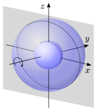
Figure 2: An illustration of the qubit HW channel ($d=2$). The Bloch sphere is shrunk by a factor of $|\frac{2\eta-1}{3}|$, with the state reflected in the $x$-$z$ axis for $\frac{2\eta-1}{3}>0$, and rotated by $\pi$ around the $y$ axis for $\frac{2\eta-1}{3}<0$.

III Relative entropy distances

An important functional of two quantum states $\rho$ and $\sigma$ is their relative entropy, which is defined as

$$S(\rho||\sigma)=\mathrm{Tr}\left(\rho\mathrm{log}_{2}\rho-\rho\mathrm{log}_{2}\sigma\right).$$ (9)

This is the basis for defining relative entropy distances. Given any compact and convex set of states $S$ (containing the maximally mixed state), the relative entropy distance of a state $\rho$ from this set is defined as Horos

$$E_{S}\left(\rho\right):=\inf_{\sigma\in S}S(\rho||\sigma).$$ (10)

This is known to be asymptotically continuous Horos ; Donald . One possible choice for $S$ is the set of separable (SEP) states, in which case we have the REE RMPrelent ; VedFORMm ; Pleniom

$$E_{R}\left(\rho\right):=\inf_{\sigma\in\mathrm{Sep}}S(\rho||\sigma).$$ (11)

Another possible choice is the set of PPT states, in which case we have the relative entropy distance with respect to PPT states, which we denote by RPPT. This is defined as

$$E_{P}\left(\rho\right):=\inf_{\sigma\in\mathrm{PPT}}S(\rho||\sigma),$$ (12)

which coincides with the Rains’ bound Rains ; Rains2 when $\rho$ is a Werner state, as shown in Ref. Audenert . Recall that a PPT state $\sigma$ is such that $\sigma^{\mathrm{PT}}$ has non-negative eigenvalues (where $\mathrm{PT}$ is transposition over the second subsystem only). This is a necessary condition for $\sigma$ to be separable, but is not sufficient, unless $\sigma$ is a 2-qubit or qubit-qutrit state. Thus, in general, we have

$$E_{P}(\rho)\leq E_{R}(\rho).$$ (13)

Both the measures here defined are subadditive, i.e., they have the following property under tensor product,

$$E_{R(P)}^{2}(\rho):=\frac{E_{R(P)}\left(\rho^{\otimes 2}\right)}{2}\leq E_{R(P)}\left(\rho\right).$$ (14)

It was shown that there exist states which are strictly subadditive ($<$). In fact, for $d>2$, Ref. VolWer proved that

$$E_{R(P)}^{2}\left(W_{-1,d}\right)<E_{R(P)}(W_{-1,d}).$$ (15)

This motivates the definition of the regularised quantities

$$E_{R(P)}^{\infty}\left(\rho\right)=\lim_{n\rightarrow\infty}\frac{E_{R(P)}\left(\rho^{\otimes n}\right)}{n}\leq E_{R(P)}\left(\rho\right),$$ (16)

i.e., the regularised REE $E_{R}^{\infty}$ and RPPT $E_{P}^{\infty}\leq E_{R}^{\infty}$.

For an entangled Werner state, the closest separable and PPT state (for one copy) is the boundary Werner separable state $W_{0,d}$, so that VolWer

$$E_{R(P)}\left(W_{\eta,d}\right)$$ (17)

$$=\begin{cases}0&\text{ if }\eta\geq 0,\\ \frac{1+\eta}{2}\mathrm{log}_{2}\left(1+\eta\right)+\frac{1-\eta}{2}\mathrm{log}_{2}\left(1-\eta\right)&\text{ if }\eta\leq 0.\end{cases}$$

Note that the one-copy quantity $E_{R(P)}\left(W_{\eta,d}\right)$ does not depend on the dimension $d$. Then, for Werner states, the regularised RPPT $E_{P}^{\infty}$ is known Audenert and reads

$$E_{P}^{\infty}\left(W_{\eta,d}\right)$$ (18)

$$= \begin{cases}0&\text{ if }\eta\geq 0,\\ \frac{1+\eta}{2}\mathrm{log}_{2}\left(1+\eta\right)+\frac{1-\eta}{2}\mathrm{log}_{2}\left(1-\eta\right)&\text{ if }-\frac{2}{d}\leq\eta\leq 0,\\ \mathrm{log}_{2}\left(\frac{d+2}{d}\right)+\frac{1+\eta}{2}\mathrm{log}_{2}\left(\frac{d-2}{d+2}\right)&\text{ if }\eta\leq-\frac{2}{d}.\end{cases}$$

From the previous equation, we see that we have strict subadditivity $E_{P}^{\infty}\left(W_{\eta,d}\right)<E_{P}\left(W_{\eta,d}\right)$ in the region $\eta<-2/d$. Note that, in the region $-2/d\leq\eta\leq 0$, the REE is additive, and that the REE, the RPPT, and their regularised versions all coincide. In fact, using the previous results, one has

$$E_{R}\left(W_{\eta,d}\right) =E_{P}\left(W_{\eta,d}\right)=E_{P}^{\infty}\left(W_{\eta,d}\right)$$

$$\leq E_{R}^{\infty}\left(W_{\eta,d}\right)\leq E_{R}\left(W_{\eta,d}\right).$$ (19)

IV Relative entopy distance of a two-copy Werner state

One of the results of Ref. VolWer was to show that the closest state $\sigma$ minimizing $E_{R(P)}(W_{\eta,d}^{\otimes n})$ is invariant under the following transformation

$$U_{d}^{1}\otimes U_{d}^{1}\otimes\ldots U_{d}^{n}\otimes U_{d}^{n}\left(\sigma\right)(U_{d}^{1}\otimes U_{d}^{1}\otimes\ldots U_{d}^{n}\otimes U_{d}^{n})^{\dagger},$$ (20)

where each $U_{d}^{i}\otimes U_{d}^{i}$ acts on the $d\times d$ Hilbert space occupied by the $i^{\mathrm{th}}$ copy of $W_{\eta,d}$. States which are invariant under this action are of the form

$$\sigma_{\mathbf{x}}^{n} =x_{0}W_{-1,d}^{\otimes n}$$

$$+\frac{x_{1}}{n}\left(W_{-1,d}^{\otimes n-1}\otimes W_{1,d}+\ldots W_{1,d}\otimes W_{-1,d}^{\otimes n-1}\right)$$

$$+\ldots+\frac{x_{k}}{\binom{n}{k}}\left(W_{-1,d}^{n-k}\otimes W_{1,d}^{k}\ldots W_{1,d}^{k}\otimes W_{-1,d}^{n-k}\right)$$

$$+\ldots+x_{n}W_{1,d}^{\otimes n},$$ (21)

where $\mathbf{x}=\left(x_{0},x_{1},\ldots,x_{n}\right)^{T}$ is a vector of probabilities, i.e., $x_{i}\geq 0$ and $\sum_{i=0}^{n}x_{i}=1$. We also have an explicit condition of $\mathbf{x}$ to ensure that $\sigma_{\mathbf{x}}^{n}$ is PPT. This is Audenert

$$\left(\begin{array}[c]{cc}-1&1\\ 1&\frac{d-1}{d+1}\end{array}\right)^{\otimes n}\mathbf{x^{\prime}}\geq 0,$$ (22)

where

$$\mathbf{x^{\prime}}=\left(x_{0},\overset{n}{\overbrace{\frac{x_{1}}{n},\ldots,\frac{x_{1}}{n}},}\ldots\overset{\binom{n}{k}}{\overbrace{\frac{x_{k}}{\binom{n}{k}},\ldots,\frac{x_{k}}{\binom{n}{k}}}},\ldots x_{n}\right)^{T}.$$ (23)

For general $n$, it is not known if the PPT states $\sigma_{\mathbf{x}}^{n}$ satisfying Eq. (22) are separable. However, they are known to be equivalent for $n=2$ VolWer , in which case Eq. (22) simplifies to

$$1-2x_{1} \geq 0,$$ (24)

$$(d-1)-2dx_{0}+(2-d)x_{1} \geq 0,$$ (25)

$$(d-1)^{2}+4dx_{0}+2(d-1)x_{1} \geq 0,$$ (26)

where we have eliminated the dependent variable $x_{2}$. This means that, for two copies ($n=2$), the state $\sigma_{\mathbf{x}}^{2}$ is the closest state for the minimization of both $E_{P}(W_{\eta,d}^{\otimes 2})$ and $E_{R}(W_{\eta,d}^{\otimes 2})$. Let us compute the latter quantity.

Assuming the basis where the single-copy Werner state is diagonal, we may write

$$S\left(W_{\eta,d}^{\otimes n}||\sigma_{\mathbf{x}}^{n}\right) =\sum_{i=0}^{n}y_{i}\mathrm{log}_{2}\left(\frac{y_{i}}{x_{i}}\right),$$ (27)

$$y_{i} =\frac{\binom{n}{i}(1-\eta)^{n-i}(1+\eta)^{i}}{2^{n}}.$$ (28)

Therefore, for $n=2$ and in the region $\eta\leq-\frac{2}{d}$, we derive

$$E_{R}^{2}\left(W_{\eta,d}\right):=\frac{E_{R}\left(W_{\eta,d}^{\otimes 2}\right)}{2}=\min_{x_{0},x_{1}}\left\{\frac{(1-\eta)^{2}}{8}\mathrm{log}_{2}\frac{(1-\eta)^{2}}{4x_{0}}\right.$$

$$+\frac{(1-\eta)(1-\eta)}{4}\mathrm{log}_{2}\frac{(1-\eta)(1-\eta)}{2x_{1}}$$

$$\left.+\frac{(1+\eta)^{2}}{8}\mathrm{log}_{2}\frac{(1+\eta)^{2}}{4\left(1-x_{0}-x_{1}\right)}\right\},$$ (29)

where

$$1-2x_{1} \geq 0,$$ (30)

$$(d-1)-2dx_{0}+(2-d)x_{1} \geq 0,$$ (31)

$$(d-1)^{2}+4dx_{0}+2(d-1)x_{1} \geq 0,$$ (32)

$$x_{0}+x_{1} \leq 1.$$ (33)

We can use Lagrangian optimisation methods to solve this problem. Let us set

$$\theta :=d^{4}\left(\eta^{2}+1\right)^{2}-4d^{3}\eta\left(\eta^{2}-3\right)$$ (34)

$$-4d^{2}\left(\eta^{4}+3\eta^{2}-1\right)+8d\eta\left(\eta^{2}-3\right)+4\left(\eta^{2}+1\right)^{2},$$

then we compute

$$x_{0} =\frac{d^{2}\left(\eta^{2}+1\right)+\sqrt{\theta}-2d(\eta-2)-2\eta^{2}-2}{8d(d+2)},$$ (35)

$$x_{1} =-\frac{d^{2}\left(\eta^{2}-3\right)+\sqrt{\theta}-2d\eta-2\eta^{2}+6}{4\left(d^{2}-4\right)}.$$ (36)

The comparison between the one-copy REE $E_{R}(W_{\eta,d})$ of Eq. (17) and the two-copy REE $E_{R}^{2}\left(W_{\eta,d}\right)$ of Eq. (29) is shown in Fig. 3. While $E_{R}(W_{\eta,d})$ does not depend on the dimension $d$, we see that the two-copy REE considerably decreases for increasing $d>2$.

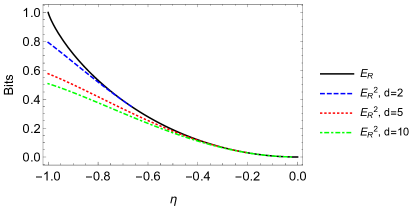
Figure 3: Comparison between the one-copy REE $E_{R}$ and the two-copy REE $E_{R}^{2}$ of a Werner state $W_{\eta,d}$, for varying dimension $d>2$. In particular, we consider here $\eta\leq 0$ which includes the subadditivity region $\eta<-2/d$.

V Two-way assisted capacities of the Holevo-Werner channels

V.1 Weak converse bounds based on the relative entropy distances

We now combine the results in the previous section with the methods of Ref. Stretching to bound the two-way capacities of the HW channels. According to Ref. Stretching , the secret-key capacity $K$ of a teleportation covariant channel $\mathcal{E}$ is upper bounded by the regularised REE of its Choi Matrix $\chi_{\mathcal{E}}$, i.e.,

$$K\left(\mathcal{E}\right)\leq E_{R}^{\infty}\left(\chi_{\mathcal{E}}\right).$$ (37)

Therefore, for an HW channel $\mathcal{W}_{\eta,d}$, we may write the upper bound

$$K(\mathcal{W}_{\eta,d})\leq E_{R}^{\infty}\left(W_{\eta,d}\right),$$ (38)

by using its corresponding Werner state $W_{\eta,d}$. From the previous section, we have that, for $\eta<-2/d$ we may write the following strict inequality

$$K(\mathcal{W}_{\eta,d})\leq E_{R}^{2}\left(W_{\eta,d}\right)<E_{R}\left(W_{\eta,d}\right),$$ (39)

so that the one-copy (single-letter) REE bound is strictly loose. This shows that the regularised REE is needed to tightly bound (and possibly establish) the secret-key capacity of an HW channel. As shown in Fig. 3, the improvement of $E_{R}^{2}$ over $E_{R}$ is better and better for increasing dimension $d$.

Let us now consider the two-way quantum capacity $Q_{2}$, which is also known to be equal to the channel’s two-way entanglement distribution capacity $D_{2}$. In Appendix A, we provide a general proof of the following.

Lemma 1 (Channel’s RPPT bound)

For a teleportation covariant channel $\mathcal{E}$, we may write

$$Q_{2}(\mathcal{E})\leq E_{P}^{\infty}\left(\chi_{\mathcal{E}}\right),$$ (40)

where the Choi matrix $\chi_{\mathcal{E}}$ and the RPPT $E_{P}^{\infty}$ are meant to be asymptotic if $\mathcal{E}$ is a continuous-variable channel. In particular, $E_{P}^{\infty}\left(\chi_{\mathcal{E}}\right)$ becomes the regularisation of

$$E_{P}\left(\chi_{\mathcal{E}}\right):=\inf_{\sigma^{\mu}}\underset{\mu\rightarrow+\infty}{\lim\inf}S(\chi_{\mathcal{E}}^{\mu}||\sigma^{\mu}),$$ (41)

where: $\chi_{\mathcal{E}}^{\mu}:=\mathcal{I}\otimes\mathcal{E}(\Phi^{\mu})$ is defined on a two-mode squeezed vacuum state $\Phi^{\mu}$ with energy $\mu$, and $\sigma^{\mu}$ is a sequence of PPT states converging in trace norm, i.e., such that $\left\|\sigma^{\mu}-\sigma\right\|\overset{\mu}{\rightarrow}0$ for some PPT state $\sigma$.

By applying the bound of Eq. (40) to an HW channel $\mathcal{W}_{\eta,d}$, we may write

$$Q_{2}(\mathcal{W}_{\eta,d})\leq E_{P}^{\infty}\left(W_{\eta,d}\right),$$ (42)

where the right hand side is computed as in Eq. (18). Of course we may also write

$$Q_{2}(\mathcal{W}_{\eta,d})\leq E_{R}^{2}\left(W_{\eta,d}\right)\leq E_{R}\left(W_{\eta,d}\right)=E_{P}\left(W_{\eta,d}\right).$$ (43)

The bounds in Eqs. (42) and (43) are shown and compared in Fig. 4 for a HW channel in dimension $d=5$.

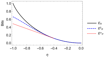
Figure 4: Weak converse upper bounds for the two-way quantum capacity $Q_{2}$ of the HW channel $\mathcal{W}_{\eta,5}$ (dimension $d=5$). We compare the one-copy REE bound $E_{R}(=E_{P})$, the two-copy REE bound $E_{R}^{2}\left(=E_{P}^{2}\right)$, and the regularised RPPT bound $E_{P}^{\infty}$, which is the tightest. Note that $E_{R}$ and $E_{R}^{2}$ also bound the secret-key capacity $K$ of the channel.

V.2 Weak converse bounds based on the squashed entanglement

Whilst the relative entropy distances provide useful upper bounds, we may also consider other functionals. In particular, we may consider the squashed entanglement. For an arbitrary bipartite state $\rho_{AB}$, this is defined as squash ; HayashiINTRO

$$E_{sq}(\rho_{AB}):=\frac{1}{2}\min_{\rho_{ABE}^{\prime}\in\Omega_{AB}}S(A:B|E),$$ (44)

where $\Omega_{AB}$ is the set of density matrices $\rho_{ABE}^{\prime}$ satisfying $\mathrm{Tr}_{E}(\rho_{ABE}^{\prime})=\rho_{AB}$, and $S(A:B|E)$ is the conditional mutual information

$$S(A:B|E):=S(\rho_{AE}^{\prime})+S(\rho_{BE}^{\prime})-S(\rho_{E})-S(\rho_{ABE}),$$ (45)

with $S(...)$ being the Von Neumann entropy NielsenChuang .

The squashed entanglement can be combined with teleportation stretching Stretching to provide a single-letter bound to the secret-key capacity. In fact, it satisfies all the required conditions. It normalises, so that $E_{sq}(\phi_{m})\geq mR_{m}$ for a private state $\phi_{m}$ with $mR_{m}$ private bits squash . It is continuous, and monotonic under LOCC squash . Furthermore, it is additive over tensor-product states, which means that there is no need to regularize over many copies. For a teleportation covariant dicrete-variable channel $\mathcal{E}$, we may therefore write

$$K(\mathcal{E})\leq E_{sq}(\chi_{\mathcal{E}}).$$ (46)

This is a direct consequence of Proposition 6 of Ref. Stretching , according to which we may write

$$K(\mathcal{E})=K(\chi_{\mathcal{E}}),$$ (47)

where the latter is the distillable key of the Choi matrix $\chi_{\mathcal{E}}$. Then, using Ref. squash , we may write $K(\chi_{\mathcal{E}})\leq E_{sq}(\chi_{\mathcal{E}})$, which leads to Eq. (46) ProvaCV .

However, there is some difficulty in optimizing over $\rho_{ABE}^{\prime}$ such that $\mathrm{Tr}_{E}(\rho_{ABE}^{\prime})=\chi_{\mathcal{E}}$, since the dimension of the environment system $E$ is generally unbounded. In order to provide an analytical upper bound, we simply choose the purification $\tilde{\chi}_{\mathcal{E}}$ of $\chi_{\mathcal{E}}$. In the case of an HW channel $\mathcal{E}=\mathcal{W}_{\eta,d}$, we have $\chi_{\mathcal{E}}=W_{\eta,d}$ and we may write

$$K(\mathcal{W}_{\eta,d}) \leq E_{sq}(W_{\eta,d})$$

$$\leq\tilde{E}_{sq}(W_{\eta,d}):=\frac{1}{2}S(A:B|E)_{\tilde{W}_{\eta,d}}$$

$$=\log_{2}d+\frac{1+\eta}{4}\log_{2}\frac{1+\eta}{d(d+1)}$$

$$+\frac{1-\eta}{4}\log_{2}\frac{1-\eta}{d(d-1)},$$ (48)

which is positive only if $\eta\leq 0$.

We can find a further upper bound by exploiting the convexity property of the squashed entanglement. First note that

$$W_{\eta,d} =\frac{\left(d-\eta\right)\mathbb{I}+\left(d\eta-1\right)\mathbb{F}}{d^{3}-d}$$

$$=\left(1+\eta\right)W_{0,d}+\left(-\eta\right)W_{-1,d},$$ (49)

which means that for $-1\leq\eta\leq 0$ the state $W_{\eta,d}$ can be written as a convex combination of the separable state $W_{0,d}$ and the extremal Werner state $W_{-1,d}$. Second, note that we have $E_{sq}\left(W_{0,d}\right)=0$ (since it is a separable state) and, for the extremal state, we may write entanglementantisymmetricstate

$$E_{sq}\left(W_{-1,d}\right)\leq\begin{cases}\log_{2}\left(\frac{d+2}{d}\right)&\text{if }d\text{ even,}\\ \frac{1}{2}\log_{2}\left(\frac{d+3}{d-1}\right)&\text{if }d\text{ uneven.}\end{cases}$$ (50)

Using the convexity property of the squashed entanglement squash

$$E_{sq}\left[p\rho_{1}+(1-p)\rho_{2}\right]$$

$$\leq pE_{sq}\left(\rho_{1}\right)+(1-p)E_{sq}\left(\rho_{2}\right),$$ (51)

we find that

$$K(\mathcal{W}_{\eta,d})\leq E_{sq}\left(W_{\eta,d}\right)\leq E_{sq}^{\ast}\left(W_{\eta,d}\right),$$ (52)

where we define

$$E_{sq}^{\ast}\left(W_{\eta,d}\right)=\begin{cases}-\eta\log_{2}\left(\frac{d+2}{d}\right)&\text{if }d\text{ even,}\\ -\frac{\eta}{2}\log_{2}\left(\frac{d+3}{d-1}\right)&\text{if }d\text{ uneven,}\end{cases}$$ (53)

for $-1\leq\eta\leq 0$ and zero otherwise.

These bounds are compared in Fig. 5 for the case of an HW channel with dimension $d=4$. We can see that one bound is better than another depending on the value of $\eta$. In particular, the secret-key capacity is in the gray area of Fig. 5(a) or, equivalently, below the composition of bounds shown in Fig. 5(b).

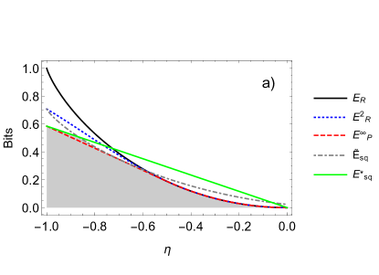
Figure 5: Comparison of the capacity bounds for the HW channel $\mathcal{W}_{\eta,4}$. (a) The regularised RPPT bound $E_{P}^{\infty}$ is the lowest (red-dashed) curve and bounds the two-way quantum capacity $Q_{2}$ of the channel. The secret-key capacity of the channel $K$ is in the gray area. Depending on the value of $\eta$, this is upper-bounded by the two-copy REE bound $E_{R}^{2}(=E_{P}^{2})$ (better than $E_{R}(=E_{P})$) or by the squashed entanglement bounds $\tilde{E}_{sq}$ and $E_{sq}^{\ast}$. We see that $\tilde{E}_{sq}$ coincides with $E_{R}^{2}$ for $\eta=-1$. (b) We show the competing upper bounds for the secret-key capacity $K$ of the HW channel $\mathcal{W}_{\eta,4}$, explicitly drawing which bound is better at which value of $\eta$. We see that the squashed entanglement bounds perform better at lower $\eta$, while the REE bounds are better for higher $\eta$.

VI Holevo-Werner Repeater Chains and Quantum Networks

VI.1 Repeater chains

In this section, we apply the results of Ref. ref1 to bound the end-to-end capacities of quantum networks in which the edges between nodes are HW channels. First, we consider the simplest multi-hop quantum network which consists of a linear chain of $N$ repeaters between the two end-parties. Such a set up is depicted in Fig. 6.

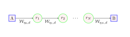
Figure 6: Alice (A) and Bob (B) are connected by $N$ quantum repeaters $r_{1}$,…, $r_{N}$ in a linear chain; each connection (edge) in the chain is a $d$ dimension HW channel with a generally-different parameter $\eta_{i}$.

For a linear chain of $N$ quantum repeaters, whose $N+1$ connecting channels $\{\mathcal{E}_{i}\}_{i=0}^{N}$ are teleportation covariant, we have that the secret capacity $K$ of the chain and its two-way quantum capacity $Q_{2}$ are bounded by ref1

$$Q_{2} \leq K\leq\min_{i}E_{R}^{\infty}\left(\chi_{\mathcal{E}_{i}}\right)$$

$$\leq\min_{i}E_{R}^{2}\left(\chi_{\mathcal{E}_{i}}\right)\leq\min_{i}E_{R}\left(\chi_{\mathcal{E}_{i}}\right),$$ (54)

with $\chi_{\mathcal{E}_{i}}$ the Choi matrix of the $i^{\text{th}}$ channel. Similarly, we may use the squashed entanglement and write ref1

$$Q_{2} \leq K\leq\min_{i}E_{sq}\left(\chi_{\mathcal{E}_{i}}\right)$$

$$\leq\min\{\min_{i}\tilde{E}_{sq}\left(\chi_{\mathcal{E}_{i}}\right),\min_{i}E_{sq}^{\ast}\left(\chi_{\mathcal{E}_{i}}\right)\}.$$ (55)

In general, we may write

$$Q_{2}\leq K\leq\min_{E}\min_{i}E\left(\chi_{\mathcal{E}_{i}}\right),$$ (56)

where the bound is also minimized over the type of entanglement measure. In particular, we may consider the “ideal” set $E\in\{E_{R}^{\infty},E_{sq}\}$ or the “computable” one $E\in\{E_{R}^{2}\leq E_{R},\tilde{E}_{sq},E_{sq}^{\ast}\}$. Then, if the task of the parties is to transmit qubits (or distill ebits), we may use the regularised RPPT and write ref1

$$Q_{2}=D_{2}\leq\min_{i}E_{P}^{\infty}\left(\chi_{\mathcal{E}_{i}}\right).$$ (57)

Let us apply these results to a linear repeater chain connected by $N+1$ iso-dimensional HW channels $\left\{\mathcal{W}_{\eta_{i},d}\right\}=\left\{\mathcal{W}_{\eta_{0},d},\ldots,\mathcal{W}_{\eta_{N},d}\right\}$, i.e., with the same dimension $d$ but generally different $\eta$’s. We may simplify the previous bounds ($E_{R}$, $E_{R}^{2}$, $\tilde{E}_{sq}$, $E_{sq}^{\ast}$, and $E_{P}^{\infty}$) by exploiting the fact that they are monotonically decreasing in $\eta$, so that the maximum value $\eta_{\text{max}}:=\max\left\{\eta_{i}\right\}$ determines the bottleneck of the chain, i.e., $\min_{i}E=E(W_{\eta_{\text{max}},d})$. In particular, for $\eta_{\text{max}}\geq 0$, we certainly have $Q_{2}=D_{2}=K=0$ because $E_{R}(W_{\eta_{\text{max}}\geq 0,d})=0$ from Eq. (17). By contrast, if $\eta_{\text{max}}\leq 0$, then we may write the following bounds for the secret-key capacity and two-way quantum capacity of the repeater chain

$$K\left(\left\{\mathcal{W}_{\eta_{i},d}\right\}\right) \leq\min_{E}E\left(W_{\eta_{\text{max}},d}\right),$$ (58)

$$Q_{2}\left(\left\{\mathcal{W}_{\eta_{i},d}\right\}\right) \leq E_{P}^{\infty}\left(W_{\eta_{\text{max}},d}\right).$$ (59)

In Eq. (58), the optimal entanglement measure $E$ can be computed from the set $\{E_{R}^{2}\leq E_{R},\tilde{E}_{sq},E_{sq}^{\ast}\}$, where $E_{R}$ is given in Eq. (17), $E_{R}^{2}$ in Eq. (29), $\tilde{E}_{sq}$ in Eq. (48), $E_{sq}^{\ast}$ in Eq. (53). In Eq. (59), we compute $E_{P}^{\infty}$ from Eq. (18).

VI.2 Single-path routing in quantum networks

We may then extend the results to an arbitrary quantum network, where there exist many possible paths between the two end-parties, Alice and Bob. Assuming single-path routing, a single chain of repeaters is used for each use of the network and this may differ from use to use. For a network connected by teleportation covariant channels, we may bound the single-path secret-key capacity of the network as ref1

$$K\leq\min_{C}E(C),~{}E(C):=\max_{\mathcal{E}\in\tilde{C}}E(\chi_{\mathcal{E}}),$$ (60)

where $E$ is a suitable entanglement measure, here to be optimized in $\{E_{R},E_{sq}\}$ remark , and $\tilde{C}$ is a “cut-set” associated with the cut Slepian ; netflow .

The cut-set $\tilde{C}$ can be described as a set of channels such that, if those channels were removed by the cut, then the network would be bi-partitioned, with Alice and Bob in separate sets of nodes. Therefore the meaning of Eq. (60) is that: (i) we perform an arbitrary cut $C$ of the network; (ii) we consider the channels $\mathcal{E}$ in the cut-set $\tilde{C}$; (iii) we compute the entanglement measure $E$ of their Choi matrices $\chi_{\mathcal{E}}$; (iv) we take the maximum so as to compute $E(C)$; (v) we finally minimize over all the possible Alice-Bob cuts $C$ of the network.

In the case of a quantum network connected by HW channels, we may the following bound for the single-path secret-key capacity

$$K\leq\min_{C}\max_{\mathcal{W}_{\eta,d}\in\tilde{C}}E(W_{\eta,d}).$$ (61)

If the HW channels are iso-dimensional (as in the example of Fig. 7), then we may simplify the previous bound into the following

$$K\leq\min_{C}E(W_{\eta_{\text{min}(C)},d}),$$ (62)

where $\eta_{\text{min}(C)}$ is the smallest expectation parameter belonging to the cut-set $\tilde{C}$. In particular, we may also miminize $E$ over $\{E_{R},\tilde{E}_{sq},E_{sq}^{\ast}\}$ by computing $E_{R}$ as in Eq. (17), $\tilde{E}_{sq}$ as in Eq. (48), and $E_{sq}^{\ast}$ as in Eq. (53).

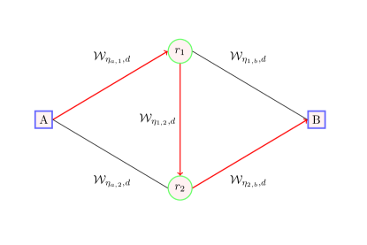
Figure 7: Alice (A) and Bob (B) as end-nodes of a diamond network connected by iso-dimensional HW channels with generally-different expectation parameters $\eta$. In red we show a possible path between the end-nodes.

VI.3 Multi-path routing in quantum networks

Finally we may also consider multipath routing. In this case, each use of the network corresponds to a simultaneous use of all the channels, allowing for simultaneous pathways between Alice and Bob (e.g., see Fig. 8). This is also known as a flooding protocol flooding and represents a crucial requirement in order to extend the max-flow/min-cut theorem Harris ; Ford ; ShannonFLOW to the quantum setting ref1 .

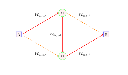
Figure 8: Example of multipath routing in a diamond network (with iso-dimensional HW channels). With respect to Fig. 7 all the channels are used in a single use of the network (flooding protocol). Dashed lines represent the advantage over the previous single-path routing protocol.

For a network connected by teleportation-covariant channels, the multi-path secret-key capacity $K^{\text{m}}\geq K$ is bounded as ref1

$$K^{\text{m}} \leq\min_{C}\Sigma^{\infty}(C)\leq\cdots\leq\min_{C}\Sigma^{r}(C)$$

$$\leq\cdots\leq\min_{C}\Sigma^{1}(C),$$ (63)

where, for any integer $r=1,\cdots,\infty$,

$$\Sigma^{r}(C):=\sum_{\mathcal{E}\in\tilde{C}}E^{r}(\chi_{\mathcal{E}}).$$ (64)

and $E^{r}$ is a suitable $r$-copy entanglement measure. In particular, we may optimize over the multi-copy REE $E^{r}=E_{R}^{r}$ or the squashed entanglement $E^{r}=E_{sq}$ (the latter being additive). For the multipath two-way quantum capacity, we may correspondingly write

$$Q_{2}^{\text{m}}\leq\min_{C}\Sigma_{P}^{\infty}(C)\leq\cdots\leq\min_{C}\Sigma_{P}^{1}(C),$$ (65)

where

$$\Sigma_{P}^{r}(C):=\sum_{\mathcal{E}\in\tilde{C}}E_{P}^{r}(\chi_{\mathcal{E}}),$$ (66)

and $E_{P}^{r}$ is the $r$-copy RPPT.

For a network connected by HW channels $\mathcal{W}_{\eta,d}$, we may specify the previous bounds to one- and two-copy REE, so that we may write

$$K^{\text{m}}\leq\min_{C}\sum_{\mathcal{W}_{\eta,d}\in\tilde{C}}E_{R}^{2}(W_{\eta,d})\leq\min_{C}\sum_{\mathcal{W}_{\eta,d}\in\tilde{C}}E_{R}(W_{\eta,d}),$$ (67)

where $E_{R}$ is in Eq. (17), and $E_{R}^{2}$ in Eq. (29). The first bound in Eq. (67) is certainly tighter than the second one if the channels have $\eta<-2/d$. More generally, we write

$$K^{\text{m}}\leq\min_{E}\min_{C}\sum_{\mathcal{W}_{\eta,d}\in\tilde{C}}E(W_{\eta,d}),$$ (68)

where $E$ is minimized in the computable set $\{E_{R}^{2}\leq E_{R},\tilde{E}_{sq},E_{sq}^{\ast}\}$. Finally, we may write

$$Q_{2}^{\text{m}}\leq\min_{C}\sum_{\mathcal{W}_{\eta,d}\in\tilde{C}}E_{P}^{\infty}(W_{\eta,d})\leq\min_{C}\sum_{\mathcal{W}_{\eta,d}\in\tilde{C}}E_{P}(W_{\eta,d}),$$ (69)

where $E_{P}$ is in Eq. (17) and $E_{P}^{\infty}$ in Eq. (18). The first bound in Eq. (69) is computable from the regularised RPPT in Eq. (18) and is certainly strictly tigther than the second bound if the channels have $\eta<-2/d$.

VII Conclusions

In this work we have considered quantum and private communication over the class of (teleportation-covariant) Holevo-Werner channels. We have computed suitable upper bounds for their two-way assisted capacities in terms of relative entropy distances, i.e., the relative entropy of entanglement (REE) and its variant with respect to PPT states (RPPT), and also in terms of the squashed entanglement (using the identity isometry and then the convexity property).

We have shown that there is a general competing behaviour between these bounds, so that an optimization over the entanglement measure is in order. These calculations were done not only for point-to-point communication, but also for chains of quantum repeaters and, more generally, quantum networks under different types of routings.

In all cases, we have also pointed out the subadditivity behaviour of the REE and RPPT bounds, so that their two-copy and regularised versions perform strictly better than their simpler one-copy expressions, under suitable conditions of the parameters. From this point of view, our paper clearly shows how the subadditivity properties of the Werner states can be fully mapped to the corresponding Holevo-Werner channels in configurations of adaptive quantum and private communication.

Acknowledgements.–This work has been supported by the EPSRC via the ‘UK Quantum Communications Hub’ (EP/M013472/1) and by the Innovation Fund Denmark (Qubiz project). The authors would like to thank David Elkouss for feedback.

Appendix A Proof of the RPPT bound in Lemma 1 at any dimension

A.1 Discrete-variable channels

To get the result for finite dimension, we may apply an heuristic argument of reduction into entanglement distillation B2main (suitably extended from Pauli channels to teleportation-covariant channels). This gives $Q_{2}(\mathcal{E})=D_{2}(\chi_{\mathcal{E}})$, where the latter is the two-way distillability of the Choi matrix $\chi_{\mathcal{E}}$. Then, we may use the fact that $D_{2}(\chi_{\mathcal{E}})\leq E_{P}^{\infty}\left(\chi_{\mathcal{E}}\right)$ (HayashiINTRO, , Sec. 8.10), therefore deriving the bound in Eq. (40) for discrete variable channels.

This bound can be proven more rigorously (and also extended to bosonic channels), by resorting to teleportation stretching Stretching , where the $n$-use output of a quantum protocol $\rho^{n}$ is directly expressed in terms of the resource states ($\chi_{\mathcal{E}}^{\otimes n}$) via a single but complicated trace-preserving LOCC $\Lambda$, i.e.,

$$\rho^{n}=\Lambda\left(\chi_{\mathcal{E}}^{\otimes n}\right).$$ (70)

Recall that, for any channel $\mathcal{E}$, we may consider an adaptive entanglement-distillation protocol $\mathcal{P}$ such that, after $n$ uses, Alice and Bob share an output state $\rho^{n}$ satisfying the trace-distance condition $||\rho^{n}-\Phi_{2}^{\otimes nR_{n}}||_{1}\leq\varepsilon$, where $\Phi_{2}^{\otimes nR_{n}}$ are $nR_{n}$ ebits. By taking the limit in $n$ and optimizing over $\mathcal{P}$, we write

$$Q_{2}(\mathcal{E})=D_{2}(\mathcal{E})=\sup_{\mathcal{P}}\lim_{n\rightarrow\infty}R_{n}.$$ (71)

Then recall the asymptotic continuity: For any pair of finite-dimensional bipartite states, $\rho$ and $\sigma$, such that $||\rho-\sigma||_{1}\leq\varepsilon$, we may write $|E_{P}(\rho)-E_{P}(\sigma)|\leq f(\varepsilon,d)$, where Horos ; Donald ; Winter

$$f(\varepsilon,d):=\frac{\varepsilon}{2}\mathrm{log}_{2}d+\left(1+\frac{\varepsilon}{2}\right)H_{2}\left(\frac{\varepsilon}{2+\varepsilon}\right),$$ (72)

with $H_{2}$ being the binary Shannon entropy Cover&Thomas and $d$ the smaller of the two subsystems’ dimensions. For any finite $d$, this function $f$ disappears as $\varepsilon\rightarrow 0$. Using this property and the normalization Rains $E_{P}(\Phi_{2}^{\otimes nR_{n}})\geq nR_{n}$, we may write

$$nR_{n}\leq E_{P}(\Phi_{2}^{\otimes nR_{n}})\leq E_{P}(\rho^{n})+f(\varepsilon,d^{nR_{n}}).$$ (73)

Next step is to apply teleportation stretching to reduce the output state $\rho^{n}$. For an adaptive protocol over a finite-dimensional teleportation-covariant channel, we may write Eq. (70) where $\chi_{\mathcal{E}}$ is the channel’s Choi matrix and $\Lambda$ is a trace-preserving LOCC Stretching . Because the RPPT is monotonic under PPT operations, it is so under the more restrictive LOCCs as $\Lambda$. Therefore, we may write $E_{P}(\rho^{n})\leq E_{P}(\chi_{\mathcal{E}}^{\otimes n})$ and Eq. (73) becomes

$$nR_{n}\leq E_{P}\left(\chi_{\mathcal{E}}^{\otimes n}\right)+f(\varepsilon,d^{nR_{n}})$$ (74)

$$=E_{P}\left(\chi_{\mathcal{E}}^{\otimes n}\right)+\frac{\varepsilon nR_{n}}{2}\mathrm{log}_{2}d$$

$$+\left(1+\frac{\varepsilon}{2}\right)H_{2}\left(\frac{\varepsilon}{2+\varepsilon}\right).$$ (75)

By re-organizing the terms in the previous inequality, we may write

$$R_{n}\leq\frac{E_{P}\left(\chi_{\mathcal{E}}^{\otimes n}\right)+\left(1+\frac{\varepsilon}{2}\right)H_{2}\left(\frac{\varepsilon}{2+\varepsilon}\right)}{n\left(1-\frac{\varepsilon}{2}\mathrm{log}_{2}d\right)}.$$ (76)

Taking the limit in $n$, we therefore get

$$\lim_{n\rightarrow\infty}R_{n}\leq\frac{E_{P}^{\infty}\left(\chi_{\mathcal{E}}\right)}{1-\frac{\varepsilon}{2}\mathrm{log}_{2}d}.$$ (77)

For $\varepsilon\rightarrow 0$ (weak converse), we obtain $\lim_{n\rightarrow\infty}R_{n}\leq E_{P}^{\infty}\left(\chi_{\mathcal{E}}\right)$ and the optimization over the protocols $\mathcal{P}$ automatically leads to the upper bound $Q_{2}(\mathcal{E})\leq E_{P}^{\infty}\left(\chi_{\mathcal{E}}\right)$ as promised in Eq. (40).

A.2 Continuous-variable channels

Thanks to the latter derivation, we can extend the bound to continuous-variable (bosonic) channels, for which the output state $\rho^{n}$ is infinite-dimensional. Following Ref. Stretching , we apply a truncation LOCC $\mathbb{T}_{d}$ at the output of the protocol $\mathcal{P}$ so that $\rho^{n,d}=\mathbb{T}_{d}(\rho^{n})$ is a finite dimensional state, epsilon-close to $nR_{n,d}$ ebits. We may then repeat the previous steps and modify Eq. (73) into

$$nR_{n,d} \leq E_{P}(\rho^{n,d})+f(\varepsilon,d^{nR_{n,d}})$$ (78)

$$\leq E_{P}(\rho^{n})+f(\varepsilon,d^{nR_{n,d}}),$$ (79)

where we exploit the monotoniticy $E_{P}(\rho^{n,d})\leq E_{P}(\rho^{n})$ in the second inequality.

Now we use the asymptotic stretching $\rho^{n}=\lim_{\mu}\Lambda(\chi_{\mathcal{E}}^{\mu\otimes n})$ in terms of the quasi-Choi matrix $\chi_{\mathcal{E}}^{\mu}:=\mathcal{I}\otimes\mathcal{E}(\Phi^{\mu})$, with $\Phi^{\mu}$ being a two-mode squeezed vacuum state with energy $\mu$. More precisely, we write

$$\left\|\rho^{n}-\Lambda(\chi_{\mathcal{E}}^{\mu\otimes n})\right\|\leq n\varepsilon_{\mu,N},$$ (80)

where $\varepsilon_{\mu,N}:=\left\|\mathcal{E}-\mathcal{E}^{\mu}\right\|_{\diamond N}$ is the channel simulation error expressed in terms of energy-constrained diamond distance between the channel $\mathcal{E}$ and its teleportation simulation $\mathcal{E}^{\mu}$ Stretching . For any finite energy $N$ of the input alphabet, we have the bounded-uniform convergence of the Braunstein-Kimble protocol, so that $\lim_{\mu}\varepsilon_{\mu,N}=0$. As a result for any $N$, we have the asymptotic convergence in trace distance

$$\lim_{\mu}\left\|\rho^{n}-\Lambda(\chi_{\mathcal{E}}^{\mu\otimes n})\right\|=0\text{.}$$ (81)

We may therefore use the lower semi-continuity of the relative entropy HolevoBOOK . In fact, we may write

$$E_{P}(\rho^{n}) =\inf_{\sigma\in\text{PPT}}S(\rho^{n}||\sigma)$$

$$\overset{(1)}{\leq}\inf_{\sigma^{\mu}}S\left[\lim_{\mu}\Lambda(\chi_{\mathcal{E}}^{\mu\otimes n})~{}||~{}\lim_{\mu}\sigma^{\mu}\right]$$

$$\overset{(2)}{\leq}\inf_{\sigma^{\mu}}\underset{\mu\rightarrow+\infty}{\lim\inf}~{}S\left[\Lambda(\chi_{\mathcal{E}}^{\mu\otimes n})~{}||~{}\sigma^{\mu}\right]$$

$$\overset{(3)}{\leq}\inf_{\sigma^{\mu}}\underset{\mu\rightarrow+\infty}{\lim\inf}~{}S\left[\Lambda(\chi_{\mathcal{E}}^{\mu\otimes n})~{}||~{}\Lambda(\sigma^{\mu})\right]$$

$$\overset{(4)}{\leq}\inf_{\sigma^{\mu}}\underset{\mu\rightarrow+\infty}{\lim\inf}~{}S\left(\chi_{\mathcal{E}}^{\mu\otimes n}~{}||~{}\sigma^{\mu}\right)$$

$$\overset{(5)}{=}E_{P}(\chi_{\mathcal{E}}^{\otimes n}),$$ (82)

where: (1)$~{}\sigma^{\mu}$ is a sequence of PPT states such that $\|\sigma-\sigma^{\mu}\|\overset{\mu}{\rightarrow}0$ for some PPT $\sigma$; (2) we use the lower semi-continuity of the relative entropy HolevoBOOK ; (3) we use that $\Lambda(\sigma^{\mu})$ are specific types of converging PPT sequences; (4) we use the monotonicity of the relative entropy under trace-preserving LOCCs; and (5) we use the definition of RPPT for asymptotic states of Eq. (41).

Combining Eqs. (79) and (82), we then derive

$$nR_{n,d,N}\leq E_{P}(\chi_{\mathcal{E}}^{\otimes n})+f(\varepsilon,d^{nR_{n,d,N}}),$$ (83)

for any $n$, $d$ and $N$. We can compute the extension of Eq. (77), which is

$$\lim_{n\rightarrow\infty}R_{n,d,N}\leq\frac{E_{P}^{\infty}\left(\chi_{\mathcal{E}}\right)}{1-\frac{\varepsilon}{2}\mathrm{log}_{2}d}.$$ (84)

For $\varepsilon\rightarrow 0$ (weak converse), we obtain $\lim_{n\rightarrow\infty}R_{n,d,N}\leq E_{P}^{\infty}\left(\chi_{\mathcal{E}}\right)$ and the optimization over the original protocols $\mathcal{P}$ automatically leads to the upper bound

$$Q_{2}(\mathcal{E}|d,N):=\sup_{\mathcal{P}}\lim_{n\rightarrow\infty}R_{n,d,N}\leq E_{P}^{\infty}\left(\chi_{\mathcal{E}}\right)~{}.$$ (85)

Since the right hand side does not depend on the input energy constraint $N$ and the output truncated dimension $d$, we may extend it to the supremum, i.e.,

$$Q_{2}(\mathcal{E})=\sup_{d,N}Q_{2}(\mathcal{E}|d,N)\leq E_{P}^{\infty}\left(\chi_{\mathcal{E}}\right).$$ (86)

References

- (1) M. A. Nielsen, and I. L. Chuang, Quantum computation and quantum information (Cambridge University Press, Cambridge, 2000).
- (2) M. Hayashi, Quantum Information: An introduction (Springer-Verlag Berlin Heidelberg, 2006).
- (3) M. Hayashi, Quantum Information Theory: Mathematical Foundation (Springer-Verlag Berlin Heidelberg, 2017).
- (4) A. Holevo, Quantum Systems, Channels, Information: A Mathematical Introduction (De Gruyter, Berlin-Boston, 2012).
- (5) C. Weedbrook et al., Rev. Mod. Phys. 84, 621 (2012).
- (6) H. J. Kimble, Nature 453, 1023–1030 (2008).
- (7) R. Van Meter, Quantum Networking (Wiley, 2014).
- (8) S. Pirandola, and S. L. Braunstein, Nature 532, 169–171 (2016).
- (9) S. Pirandola, arXiv:1601.00966 (2016).
- (10) E. Schoute, L. Mancinska, T. Islam, I. Kerenidis, and S. Wehner, arXiv:1610.05238 (2016).
- (11) M. Pant, H. Krovi, D. Towsley, L. Tassiulas, L. Jiang, P. Basu, D. Englund, and S. Guha, arXiv:1708.07142 (2017).
- (12) F. Rozpedek, K. Goodenough, J. Ribeiro, N. Kalb, V. Caprara Vivoli, A. Reiserer, R. Hanson, S. Wehner, and D. Elkouss, arXiv:1705.00043 (2017).
- (13) L. Rigovacca, G. Kato, S. Bäuml, M. S. Kim, W. J. Munro, K. Azuma, New J. Phys. 20, 013033 (2018).
- (14) C. H. Bennett and G. Brassard. Quantum cryptography: Public key distribution and coin tossing, Proceedings of IEEE International Conference on Computers, Systems and Signal Processing, 175 (1984).
- (15) A. K. Ekert, Phys. Rev. Lett. 67, 661-663 (1991).
- (16) V. Scarani, H. Bechmann-Pasquinucci, N. J. Cerf, M. Dŭsek, N. Lütkenhaus and M. Peev, Rev. Mod. Phys. 81 1391-1350 (2009).
- (17) R. Colbeck, Quantum And Relativistic Protocols For Secure Multi-Party Computation (University of Cambridge, 2006).
- (18) C. E. Shannon, The Mathematical Theory of Communication (University of Illinois Press, 1949).
- (19) T. M. Cover, and J. A. Thomas, Elements of Information Theory (Wiley, New Jersey, 2006).
- (20) A. W. Harrow, A. Hassidim, D. W. Leung, and J. Watrous, Phys. Rev. A 81, 032339 (2010).
- (21) S. Pirandola, and C. Lupo, Phys. Rev. Lett. 118, 100502 (2017).
- (22) S. Pirandola, R. Laurenza, and C. Lupo, Fundamental limits to quantum channel discrimination, arXiv:1803.02834 (2018).
- (23) K. Kravtsov et al., Phys. Rev. A 87, 062122 (2013).
- (24) D. H. Mahler et al., Phys. Rev. Lett. 111, 183601 (2013).
- (25) R. Demkowicz-Dobrzański, and L. Maccone, Phys. Rev. Lett. 113, 250801 (2014).
- (26) A. A. Berni et al., Nature Photon. 9, 577 (2015).
- (27) Z. Hou, H. Zhu, G.-Y. Xiang, C.-F. Li, and G.-C. Guo, npj Quantum Information 2, 16001 (2016).
- (28) T. P. W. Cope, and S. Pirandola, Quantum Meas. Quantum Metrol. 4, 44-52 (2017).
- (29) R. Laurenza, C. Lupo, G. Spedalieri, S. L. Braunstein, and S. Pirandola, Quantum Meas. Quantum Metrol. 5, 1-12 (2018).
- (30) C. H. Bennett, D. P. DiVincenzo, J. A. Smolin, and W. K. Wootters, Phys. Rev. A 54, 3824-3851 (1996).
- (31) M. A. Nielsen, and I. L. Chuang, Phys. Rev. Lett. 79, 321 (1997).
- (32) G. Brassard, S. L. Braunstein, and R. Cleve, Physica D 120, 43–47 (1998).
- (33) M. Horodecki, P. Horodecki, and R. Horodecki, Phys. Rev. A 99, 1888–1898 (1999).
- (34) D. Gottesman, and I. L. Chuang, Nature 402, 390–393 (1999).
- (35) G. Bowen, and S. Bose, Phys. Rev. Lett. 87, 267901 (2001).
- (36) E. Knill, R. Laflamme, and G. Milburn, Nature 409, 46–52 (2001).
- (37) R. F. Werner, J. Phys. A 34, 7081–7094 (2001).
- (38) G. Giedke, and J. I. Cirac, Phys. Rev. A 66, 032316 (2002).
- (39) P. Aliferis, and D. W. Leung, Phys. Rev. Lett. 70, 062314 (2004).
- (40) J. Niset, J. Fiurasek, and N. J. Cerf, Phys. Rev. Lett. 102, 120501 (2009).
- (41) A. Müller-Hermes, Transposition in quantum information theory (Master’s thesis, Technical University of Munich, 2012).
- (42) M. M. Wolf, Notes on “Quantum Channels & Operations” (see page 35). Available at https://www-m5.ma.tum.de/foswiki/pub/M5/Allgemeines/ MichaelWolf/QChannelLecture.pdf.
- (43) D. Leung, and W. Matthews, IEEE Trans. Info. Theory 61, 4486-4499 (2015).
- (44) S. Pirandola, R. Laurenza, C. Ottaviani and L. Banchi, Nat. Commun. 8, 15043 (2017). See also arXiv:1510.08863 and arXiv:1512.04945 (2015).
- (45) In general, a LOCC simulation of a channel is a representation of the channel where it is replaced by an LOCC (or a sequence of LOCCs) applied to the input state and a suitable resource state (which may be finite or infinite dimensional) Stretching . A preliminary version of the LOCC simulation was proposed in Ref. HoroTEL . However, because the latter does not involve sequences of LOCCs and only considers finite dimensional , it cannot simulate the amplitude damping channel, i.e., it cannot cover all the DV channels.
- (46) V. Vedral, Rev. Mod. Phys. 74, 197 (2002).
- (47) V. Vedral, M. B. Plenio, M. A. Rippin, and P. L. Knight, Phys. Rev. Lett. 78, 2275-2279 (1997).
- (48) V. Vedral, and M. B. Plenio, Phys. Rev. A 57, 1619 (1998).
- (49) K. Goodenough, D. Elkouss, and S. Wehner, New J. Phys. 18, 063005 (2016).
- (50) M. Christandl, The Structure of Bipartite Quantum States: Insights from Group Theory and Cryptography (PhD thesis, University of Cambridge, 2006).
- (51) C. H. Bennett, D. P. DiVincenzo, and J. A. Smolin, Phys. Rev. Lett. 78, 3217-3220 (1997).
- (52) C. H. Bennett, G. Brassard, C. Crepeau, R. Jozsa, A. Peres, and W. K. Wootters, Phys. Rev. Lett. 70, 1895 (1993).
- (53) S. L. Braunstein, and H. J. Kimble, Phys. Rev. Lett. 80, 869–872 (1998).
- (54) S. L. Braunstein, G. M. D’Ariano, G. J. Milburn, and M. F. Sacchi, Phys. Rev. Lett. 84, 3486-3489 (2000).
- (55) S. Pirandola et al., Nat. Photon. 9, 641-652 (2015).
- (56) R. F. Werner, and A. S. Holevo, J. Mat. Phys. 43, 4353 (2002).
- (57) M. Fannes, B. Haegeman, M. Mosonyi and D. Vanpeteghem, arXiv:quant-ph/0410195 (2004).
- (58) R. F. Werner, Phys. Rev. A 40, 4277–4281 (1989).
- (59) F. Barrett, Phys. Rev. A 65, 042302 (2002).
- (60) K. G. H. Vollbrecht, and R. F. Werner, Phys. Rev. A 64, 062307 (2001).
- (61) D. Z. Djokovic, Entropy 18, 216 (2016).
- (62) K. Horodecki, M. Horodecki, P. Horodecki, and J. Oppenheim, IEEE Trans. Inf. Theory 55, 1898 (2009).
- (63) M. Donald, and M. Horodecki, Phys. Lett. A 264, 257-260 (1999).
- (64) E. Rains, Phys. Rev. A 60, 179 (1999).
- (65) E. M. Rains, IEEE Trans. Inf. Theory 47, 2921–2933 (2001).
- (66) K. Audenaert, J. Eisert, E. Jané, M. B. Plenio, S. Virmani, and B. De Moor, Phys. Rev. Lett. 87, 217902 (2001).
- (67) The proof for continuous-variable channels is more complicated and is not reported here. It is based on a suitable extension of the squashed entanglement functional to account for asymptotic states.
- (68) M. Christandl, N. Schuch, and A. Winter, Communications in Mathematical Physics 311, 397-422 (2012).
- (69) For technical reasons connected with the proof of the single-path bound, we cannot consider multi-copy REE quantities or the regularisation in Eq. (60).
- (70) P. Slepian, Mathematical Foundations of Network Analysis (Springer-Verlag, New York, 1968).
- (71) R. K. Ahuja, T. L. Magnanti, and J. B. Orlin, Network Flows: Theory, Algorithms and Applications (Prentice Hall, 1993).
- (72) A. S. Tanenbaum, and D. J. Wetherall, Computer Networks (5th Edition, Pearson, 2010).
- (73) T. E. Harris, and F. S. Ross, Research Memorandum, Rand Corporation (1955).
- (74) L. R. Ford, and D. R. Fulkerson, Canadian Journal of Mathematics 8, 399 (1956).
- (75) P. Elias, A. Feinstein, and C. E. Shannon, IRE Trans. Inf. Theory 2, 117–119 (1956).
- (76) A. Winter, Commun. Math. Phys 347, 291-313 (2016).