Ocean tidal heating in icy satellites with solid shells

Abstract

As a long-term energy source, tidal heating in subsurface oceans of icy satellites can influence their thermal, rotational, and orbital evolution, and the sustainability of oceans. We present a new theoretical treatment for tidal heating in thin subsurface oceans with overlying incompressible elastic shells of arbitrary thickness. The stabilizing effect of an overlying shell damps ocean tides, reducing tidal heating. This effect is more pronounced on Enceladus than on Europa because the effective rigidity on a small body like Enceladus is larger. For the range of likely shell and ocean thicknesses of Enceladus and Europa, the thin shell approximation of Beuthe (2016) is generally accurate to less than about 4%. Explaining Enceladus’ endogenic power radiated from the south polar terrain by ocean tidal heating requires ocean and shell thicknesses that are significantly smaller than the values inferred from gravity and topography constraints. The time-averaged surface distribution of ocean tidal heating is distinct from that due to dissipation in the solid shell, with higher dissipation near the equator and poles for eccentricity and obliquity forcing respectively. This can lead to unique horizontal shell thickness variations if the shell is conductive. The surface displacement driven by eccentricity and obliquity forcing can have a phase lag relative to the forcing tidal potential due to the delayed ocean response. For Europa and Enceladus, eccentricity forcing generally produces greater tidal amplitudes due to the large eccentricity values relative to the obliquity values. Despite the small obliquity values, obliquity forcing generally produces larger phase lags due to the generation of Rossby-Haurwitz waves. If Europa’s shell and ocean are respectively 10 and 100 km thick, the tide amplitude and phase lag are 26.5 m and $<1$ degree for eccentricity forcing, and $<2.5$ m and $<18$ degrees for obliquity forcing. Measurement of the obliquity phase lag (e.g. by Europa Clipper) would provide a probe of ocean thickness

1 Introduction

A variety of observations suggest the presence of subsurface global oceans in icy satellites of the outer solar system, significantly increasing their appeal as habitable worlds. Jupiter’s magnetic field tilt relative to the rotation axis generates a time-varying magnetic field, and this can in turn generate an induced magnetic field on the Galilean satellites if they contain a sufficiently conducting material. Induced magnetic fields have been detected on Europa, Ganymede, and Callisto, and the conducting material has been interpreted as a subsurface, salty, ocean (Kivelson et al., 2000; Zimmer et al., 2000; Kivelson et al., 2002). Ganymede’s internal, permanent, magnetic field (Kivelson et al., 2002) and the generation of induced magnetic fields by Callisto’s ionosphere (Hartkorn and Saur, 2017) complicates the interpretation of a subsurface ocean. Recent Hubble Space Telescope observations of Ganymede’s aurora (Saur et al., 2015), which is sensitive to induced magnetic fields, favor the presence of a subsurface ocean. Saturnian satellites do not experience a strong time-varying magnetic field due to the close alignment of the magnetic field with the rotation axis, limiting the generation of induced magnetic fields. Gravity data obtained by the Cassini mission has provided strong evidence for subsurface oceans on Titan and Enceladus. These data can be used to quantify the satellite deformation in response to the time-varying forcing tidal potential using the degree-two tidal Love number, $k_{2}^{T}$. For Titan, the large $k_{2}^{T}\sim 0.6$ requires a highly deformable interior over the tidal forcing period, suggesting the presence of a global subsurface ocean (Iess et al., 2012). The large libration amplitude of Enceladus requires decoupling the outer shell from the interior, implying the presence of a global subsurface ocean (Thomas et al., 2016). We refer the reader to Nimmo and Pappalardo (2016) for a comprehensive review of observational constraints for subsurface oceans in icy satellites.

As a long-term energy source, ocean tidal heating can influence the thermal, rotational, and orbital evolution of icy satellites, and the sustainability of subsurface oceans. The thermal, rotational, and orbital evolution are coupled because tidal heating is a main energy source that depends on the rotational and orbital parameters. Previous studies have investigated various aspects of this coupled problem (e.g. Ojakangas, 1989a; Ross and Schubert, 1990; Sohl et al., 1995; Showman et al., 1997; Hussmann and Spohn, 2004; Běhounková et al., 2012). However, these studies ignore ocean tidal heating and assume that energy dissipation occurs only in solid regions. This assumption is not justified on Earth, where most of the tidal heating is generated in the oceans. As the observational evidence for subsurface oceans in icy satellites increased, more recent studies have considered ocean tidal heating (Tyler, 2008, 2009, 2011; Chen and Nimmo, 2011; Tyler, 2014; Matsuyama, 2014; Chen et al., 2014; Hay and Matsuyama, 2017). However, these studies ignore the presence of an overlying solid shell, with the exception of Beuthe (2016) who models this effect using a thin shell approximation.

In this paper, we present a new theoretical treatment for tidal heating in thin subsurface oceans that takes into account the effect of an overlying shell of arbitrary thickness. As shown below with applications to Enceladus and Europa, this is important because an overlying shell damps ocean tides, reducing tidal heating. Additionally, ocean tidal heating can generate distinct horizontal shell thickness variations and surface displacement phase lags relative to the forcing tidal potential, which has implications for spacecraft observations.

As discussed above, Enceladus’ large libration amplitude requires the presence a global subsurface ocean, and is consistent with an ocean $26-31$ km thick and a solid shell $21-26$ km thick (Thomas et al., 2016). Bayesian inversion using gravity and topography data constrains the ocean and shell thicknesses to $38\pm 4$ km and $23\pm 4$ km respectively (Beuthe et al., 2016). We assume a spherically symmetric three-layer interior structure with the parameters in Table 1 and consider a range of shell and ocean thicknesses that are consistent with these observational constraints.

The ocean and shell thicknesses of Europa are only weakly constrained. A combined ocean and shell thickness in the range of about 80 to 170 km was estimated from the mean moment of inertia inferred from gravity data, $I/(MR^{2})=0.346\pm 0.05$, where $M$ and $R$ are the satellite mass and radius (Anderson et al., 1998). The mean moment of inertia uncertainty is likely larger due to the implicit assumption of a hydrostatic ratio $J_{2}/C_{22}=10/3$ for the degree-two gravity coefficients, and the error associated with the Radau-Darwin approximation used to obtain the mean moment of inertia from the degree-two gravity coefficients (Gao and Stevenson, 2013). We assume the simplest possible interior structure with a subsurface ocean and shell, a spherically symmetric three-layer interior structure model with the parameters in Table 1, and consider a large range of shell and ocean thicknesses.

				Enceladus		Europa
Parameter		Symbol		Value
Mass		$M$		$1.08\times 10^{20}$ kg		$4.8\times 10^{22}$ kg
Radius		$R$		252.1 km		1561 km
Rotation rate		$\Omega$		$5.31\times 10^{-5}$ rad s-1		$2.05\times 10^{-5}$ rad s-1
Orbital eccentricity		$e$		0.0047		0.0094
Predicted obliquity		$\theta_{0}$		$4.5\times 10^{-4}$ degree		0.1 degree
Core shear modulus		$\mu_{c}$		$40\times 10^{9}$ Pa		$40\times 10^{9}$ Pa
Ocean density		$\rho_{o}$		$10^{3}$ kg m-3		$10^{3}$ kg m-3
Ocean thickness		$h_{o}$		38 km		100 km
Shell density		$\rho_{s}$		940 kg m-3		940 kg m-3
Shell thickness		$h_{s}$		23 km		10 km
Shell shear modulus		$\mu_{s}$		$3.5\times 10^{9}$ Pa		$3.5\times 10^{9}$ Pa
Linear drag coefficient		$\alpha$		$10^{-11}-10^{-5}$ s-1		$10^{-11}-10^{-5}$ s-1

Table 1: Model parameters for Enceladus and Europa. Given the ocean and shell thicknesses, we calculate the core density self-consistently so as to satisfy the mean density constraint.

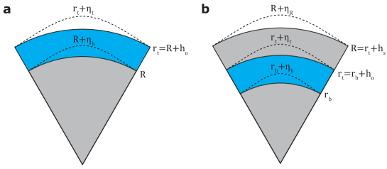
Figure 1: Comparison of radial displacements for (a) surface and (b) subsurface oceans. In both cases, the ocean thickness is $h_{o}$, and the radial tide $\eta$ is defined as the difference between the radial displacement at the top and bottom of the ocean, $\eta\equiv\eta_{t}-\eta_{b}$. For a surface ocean, the ocean bottom radius is the surface radius $R$ and the ocean top is $R+h_{o}$. For a subsurface ocean, the ocean top and bottom radii are related by $r_{t}=r_{b}+h_{o}$, the surface and ocean top radii are related by $R=r_{t}+h_{s}$, where $h_{s}$ is the overlying shell thickness, and the radial tide at the surface is $\eta_{R}$.

2 Theory

The Laplace tidal equations (LTE) describing dynamic ocean tides can be obtained from the momentum and mass conservation equations by assuming a thin, homogeneous surface ocean on a spherical planet (Lamb, 1993). For a surface or subsurface ocean, these equations can be written as

$$\partial_{t}\eta+h_{o}\nabla\cdot\mathbf{u}=0$$ (1)

and

$$\partial_{t}\mathbf{u}+2\mathbf{\mathbf{\Omega}}\times\mathbf{u}+\alpha\mathbf{u}+\frac{c_{D}}{h_{o}}|\mathbf{u}|\mathbf{u}+\nu\nabla^{2}\mathbf{u}=-\frac{1}{\rho_{o}}\nabla P+\nabla U;$$ (2)

where $h_{o}$ is a reference, uniform ocean thickness; $\mathbf{u}=(u_{\theta},\,u_{\phi})$ is the depth averaged horizontal velocity vector in spherical coordinates $\theta$ and $\phi$ (colatitude and longitude); $\alpha$, $c_{D}$, and $\nu$ are linear, bottom, and Navier-Stokes drag coefficients; and $\nabla$ is a horizontal gradient operator. That is,

$$\nabla\cdot\mathbf{u} =(r\sin\theta)^{-1}\left[\partial_{\theta}(\sin\theta u_{\theta})+\partial_{\phi}u_{\phi}\right]$$

$$\nabla U =r^{-1}\hat{\mathbf{e}}_{\theta}\partial_{\theta}U+\hat{\mathbf{e}}_{\phi}(r\sin\theta)^{-1}\partial_{\phi}U,$$ (3)

where $\mathbf{\hat{\mathbf{e}}_{\theta}}$ and $\mathbf{\hat{\mathbf{e}}_{\phi}}$ are unit vectors in the $\theta$ and $\phi$ directions (e.g., Dahlen and Tromp, 1998, Eqs. A.117, A.118 and A.141). In the mass conservation equation (1), the radial tide $\eta$ is defined as the difference between the radial displacement at the top and bottom of the ocean (Fig. 1),

$$\eta\equiv\eta_{t}-\eta_{b}\equiv\sum_{n=m}^{\infty}\sum_{m=0}^{2}\eta_{nm}Y_{nm}(\theta,\,\phi)e^{-i\omega t},$$ (4)

which we expand in spherical harmonics $Y_{nm}(\theta,\,\phi)\equiv P_{nm}(\theta)e^{im\phi}$ (C). The expansion coefficients $\eta_{nm}$ are imaginary and $P_{nm}$ is the associated Legendre function (Arfken and Weber, 1995). As described below, the forcing tidal potential is decomposed into eastward ($\omega=\Omega$) and westward ($\omega=-\Omega$) traveling components. In the momentum conservation equation (2), $\mathbf{\Omega}$ is the rotation vector, $\rho_{o}$ is the ocean density, $P$ is the radial pressure, and $U$ is the forcing potential.

The time-dependent part of the tidal forcing potential contains eccentricity and obliquity contributions, $U^{T}=U_{ecc}^{T}+U_{obliq}^{T}$, where

$$U_{ecc}^{T} =\Omega^{2}r^{2}e\left\{-\frac{3}{2}P_{20}(\cos\theta)\cos(\Omega t)+\frac{1}{8}P_{22}(\cos\theta)\left[7\cos(2\phi-\Omega t)-\cos(2\phi+\Omega t)\right]\right\}$$

$$U_{obliq}^{T} =\frac{1}{2}\Omega^{2}r^{2}\theta_{0}P_{21}(\cos\theta)\left[\cos(\phi-\Omega t)+\cos(\phi+\Omega t)\right]$$ (5)

to lowest order in eccentricity, $e$, and obliquity, $\theta_{0}$ (Tyler, 2011). Eccentricity forcing causes the total tidal bulge (static part included) to librate in longitude and to vary in amplitude, and obliquity forcing causes the tidal bulge to librate in latitude, producing time-varying ocean tides. We only consider $n=2$ contributions and ignore higher order terms because the forcing tidal potentials scale with $(r/a)^{n}$ and $r\ll a$, where $a$ is the semi-major axis of the satellite. The obliquities of Enceladus and Europa are not directly constrained by observations. We assume obliquities of $4.5\times 10^{-4}$ deg and 0.1 deg for Enceladus and Europa respectively under the assumption that tidal energy dissipation has driven the obliquities to Cassini state values (Bills, 2005; Chen and Nimmo, 2011; Baland et al., 2016).

We extend the method of Longuet-Higgins (1968) to solve the mass and momentum conservation equations for a thin ocean with an overlying incompressible elastic shell of arbitrary thickness (C). This requires ignoring bottom ($c_{D}=0$) and Navier-Stokes ($\nu=0$) drag, and in this case the dissipated energy per unit surface area and time is

$$F_{diss}=-\rho_{o}h_{o}\alpha\text{{u}$\cdot\textbf{u}$}.$$ (6)

Earth’s ocean tidal heating studies consider both linear and bottom friction drag formalisms. Egbert and Ray (2000) and Egbert and Ray (2001) assume linear drag with $\alpha^{\prime}=\alpha h_{o}\sim 0.03$ m s^-1, which yields $\alpha\sim 10^{-5}$ s^-1 assuming an average Earth ocean thickness $h_{o}\sim 4$ km. Webb (1980) assume $\alpha\sim 1/\tau$ with $\tau\sim 24-60$ hours, which also yields $\alpha\sim 10^{-5}$ s^-1. The bottom drag formalism is based on the assumption that drag arises due to turbulent flow interacting with a bottom boundary. A nominal bottom drag coefficient $\sim(2-3)\times 10^{-3}$ has been assumed to model tidal heating in the Earth (e.g., Lambeck, 1980; Jayne and St Laurent, 2001; Egbert and Ray, 2001; Green and Nycander, 2013), Titan (Sagan and Dermott, 1982), and Jovian planets (Goldreich and Soter, 1966). We can estimate a corresponding linear drag coefficient by comparing the energy flux due to linear drag (Eq. (6)) with the energy flux due to bottom drag, $F_{diss}=\rho_{o}c_{D}(\text{{u}$\cdot\textbf{u }$})^{3/2}$. This order-of-magnitude estimate yields

$$c_{D}\sim\alpha^{3/2}\left(\frac{\rho_{o}h_{o}^{3}}{F_{diss}}\right)^{1/2}.$$ (7)

There are no constraints for the linear or bottom drag coefficients in icy satellites; therefore, we consider a large range of possible values. Using the tidal heating fluxes in section 3 and the nominal value $c_{D}\sim 10^{-3}$, this estimates yields $\alpha\sim 10^{-11}$ s^-1 for eccentricity and obliquity forcing on Enceladus, $\alpha\sim 10^{-10}$ s^-1 for eccentricity forcing on Europa, and $\alpha\sim 10^{-9}$ s^-1 for obliquity forcing on Europa. We adopt these values as lower limits and the Earth value, $\alpha\sim 10^{-5}$ s^-1, as an upper limit.

Tidal heating in the solid regions of a satellite is commonly quantified by a tidal quality factor defined as $Q\equiv 2\pi E_{max}/E_{diss},$ where $E_{max}$ is the maximum energy stored in the tidal deformation and $E_{diss}$ is the energy dissipated in one cycle. For dissipation in solid regions, it is possible to calculate the elastic energy stored due to tidal deformation and the corresponding $Q$. For ocean energy dissipation, however, tidal deformation does not produce elastic energy. It is possible to introduce a tidal quality factor $Q\equiv\Omega/(2\alpha)$ for ocean tidal heating by redefining $E_{max}$ as the maximum kinetic energy of the ocean (Tyler, 2011). This definition has been used in previous ocean tidal heating studies (Tyler, 2011; Matsuyama, 2014; Chen et al., 2014; Beuthe, 2016). However, it can lead to counter-intuitive results such as decreasing energy dissipation with decreasing $Q$ (D) because the kinetic and dissipated energies are coupled (Matsuyama, 2014). Although we can introduce an alternative definition of $Q$ that is physically more intuitive (D), we do not favor its use because $Q$ is not a fundamental quantity, but a phenomenological factor whose definition depends on the particular context. This can introduce significant errors even when considering solid tides. For example, the neglect of self-gravity and hydrostatic pre-stress in the traditional relationship between $Q$ and the tidal phase delay can lead to order of magnitude errors (Zschau, 1978). The relevant quantity for computing the effect of tidal heating on the thermal, rotational, and orbital evolution is the energy dissipation rate and our thick shell theory provides a method for computing it.

The mass and momentum conservation equations (1) and (2), and the energy dissipation equation (6) are applicable to both surface and subsurface oceans; however, the pressure and forcing potential terms in the momentum conservation equation are different for each case, as described in sections 2.1 and 2.2 below.

2.1 Surface oceans

For surface oceans, the pressure at a reference radius $r$ in the ocean is $P=\rho_{o}g(r_{t}+\eta_{t}-r),$ where $r_{t}\equiv R+h_{o}$ is the constant ocean top radius (Fig. 1a) and we assume a constant gravitational acceleration $g$ in the ocean, as expected for a thin ocean. Thus, the pressure gradient term in the momentum conservation equation (2) is

$$-\frac{\nabla P}{\rho_{0}}=-g\nabla\eta_{t},$$ (8)

where we ignore density and gravitational acceleration variations. The former is justified by the assumption of an incompressible ocean, and the latter is justified by the assumption of small amplitude tides ($\eta\ll R$).

The total forcing tidal potential is given by

$$U_{nm}=\left[1+k_{n}^{T}(R)\right]U_{nm}^{T}+\left[1+k_{n}^{L}(R)\right]U_{nm}^{L},$$ (9)

where we expand the potential $U$ in spherical harmonics $U_{nm}$ and take into account the effects of ocean self-gravity and deformation of the solid regions using Love number theory (Hendershott, 1972; Matsuyama, 2014). The tidal Love number $k_{n}^{T}$ describes the response to the forcing tidal potential $U_{nm}^{T}$, and the load Love number $k_{n}^{L}$ describes the response to the ocean loading potential $U_{nm}^{L}$. We use the term ocean loading potential to refer to the gravitational potential arising from self-gravity of the tides (Lamb, 1993, p. 305, Eq. (13); Hendershott, 1972; Lambeck, 1980; Matsuyama, 2014). The Love numbers must be evaluated at the solid surface ($r=R)$ for a surface ocean (Fig. 1a) . The ocean loading potential is related to the radial tide by

$$U_{nm}^{L}=\frac{3}{(2n+1)}\frac{\rho_{o}}{\bar{\rho}}g\eta_{nm}=g\xi_{n}\eta_{nm},$$ (10)

where $\bar{\rho}$ is the mean density of the satellite and we define the degree-n density ratio

$$\xi_{n}\equiv\frac{3}{(2n+1)}\frac{\rho_{o}}{\bar{\rho}}.$$ (11)

The ocean bottom displacement (Fig. 1a) is given by

$$\eta_{nm}^{b}=h_{n}^{T}(R)U_{nm}^{T}/g(R)+h_{n}^{L}(R)U_{nm}^{L}/g(R),$$

where the displacement Love numbers $h_{n}^{T}$ and $h_{n}^{L}$ must be evaluated at the surface. Combining Eqs. (4)-(11) to eliminate the ocean loading potential yields

$$\partial_{t}\mathbf{u}+2\mathbf{\mathbf{\Omega}}\times\mathbf{u}+\alpha\mathbf{u}=-g(R)\nabla\sum_{n=m}^{\infty}\sum_{m=0}^{2}(1-\xi_{n}\gamma_{n}^{L})\eta_{nm}Y_{nm}(\theta,\,\phi)+\gamma_{2}^{T}\nabla\sum_{m=0}^{2}U_{2m}^{T}Y_{2m}(\theta,\,\phi),$$ (12)

where the tilt factors are

$$\gamma_{n}^{L} \equiv 1+k_{n}^{L}(R)-h_{n}^{L}(R)$$

$$\gamma_{2}^{T} \equiv 1+k_{2}^{T}(R)-h_{2}^{T}(R).$$ (13)

The Love numbers can be computed using the propagator matrix method (A.2) or the analytic expressions for a homogeneous, incompressible body (B.1) for the case of a uniform interior beneath the ocean.

2.2 Subsurface oceans

There are two main aspects that must be taken into account when considering ocean tidal heating in subsurface oceans. First, energy dissipation due to drag can occur at both the top and bottom of the ocean. Second, the overlying solid shell provides an additional source of pressure that resists ocean tides. In the absence of information about drag at the ocean top and bottom, the first effect can be taken into account by simply assuming a drag coefficient that is twice as large compared with the value assumed for a surface ocean (Tyler, 2014). The second effect requires a significant extension of the theory, as described below.

For a thin subsurface ocean, the total forcing potential in the momentum conservation equation (2) can be written as

$$U_{nm}=\left[(r/R)^{n}+k_{n}^{T}(r)\right]U_{nm}^{T}(R)+k_{n}^{P}(r)U_{nm}^{P}(r),$$ (14)

where $k_{n}^{T}$ and $k_{n}^{P}$ are internal, degree-$n$, tidal and pressure Love numbers (Hinderer, 1986), $U_{nm}^{T}$ are the expansion coefficients of the tidal potential, and $U_{nm}^{P}(r_{t})$ are the expansion coefficients of a pressure potential representing the dynamic part of ocean forcing on the shell. The first term in Eq. (14), $(r/R)^{n}U_{nm}^{T}(R)$, corresponds to the forcing tidal potential, and the terms $k_{n}^{T}(r)U_{nm}^{T}(R)$ and $k_{n}^{P}(r)U^{P}(r_{t})$ describe the gravitational potentials arising from the static and dynamic parts of the deformation in response to the forcing potential. This decomposition into static and dynamic components was first used to study the effect of fluid core dynamics on Earth nutations (Sasao et al., 1980, Eq. (51); Sasao and Wahr, 1981, Eq. (3.10)), and later adopted to study Earth surface gravity perturbations due to fluid core oscillations using the terminology of internal pressure Love numbers (Hinderer, 1986, Eq. (2); Hinderer and Legros, 1989, Eq. (2.9)).

The dynamic ocean pressure generates radial stress discontinuities of magnitude $\rho_{o}U_{nm}^{P}(r_{t})$ and $\rho_{o}U_{nm}^{P}(r_{b})$ at the ocean top and bottom, respectively (A.3, Eqs. (43) and (44)). In the limit of a thin ocean, $U_{nm}^{P}(r_{b})=-U_{nm}^{P}(r_{t})$, which allows us to describe pressure forcing at both the ocean top and bottom using a single Love number instead of the traditional approach of describing each forcing with a different Love number, and we choose $U_{nm}^{P}(r_{t})$ as the reference pressure potential (Appendix A.3). Under the same thin ocean approximation, Eq. (14) can be evaluated at the ocean top ($r=r_{t}$) or bottom ($r=r_{b}$), and we choose $r_{t}$ as the reference ocean radius.

In our formalism using interior Love numbers, the gravitational potential arising from the mass redistribution due to the static and dynamic ocean tide (self-gravity) is taken into account by the $k_{n}^{T}(r)U_{nm}^{T}(R)$ and $k_{n}^{P}(r)U_{nm}^{P}(r_{t})$ terms, respectively, in Eq. (14). Therefore, an additional ocean loading term is not required in the momentum conservation equation. In contrast, the subsurface ocean treatment of Beuthe (2016) using a thin shell approximation includes an ocean loading term describing ocean self-gravity in the momentum conservation equation. Despite this apparent difference in the theoretical treatment, our thick shell solutions converge to the thin shell solutions as the overlying shell thickness decreases, as shown below.

Using the tidal and pressure displacement Love numbers $h_{n}^{T}$ and $h_{n}^{P}$, the radial tides (Fig. 1b) at the surface ($r=R$), ocean top ($r=r_{t}$), and ocean bottom ($r=r_{b}$) are given by

$$\eta_{nm}^{R} =h_{n}^{T}(R)U_{nm}^{T}(R)/g(R)+h_{n}^{P}(R)U_{nm}^{P}(r_{t})/g(R)$$

$$\eta_{nm}^{t} =h_{n}^{T}(r_{t})U_{nm}^{T}(R)/g(R)+h_{n}^{P}(r_{t})U_{nm}^{P}(r_{t})/g(R)$$

$$\eta_{nm}^{b} =h_{n}^{T}(r_{b})U_{nm}^{T}(R)/g(R)+h_{n}^{P}(r_{b})U_{nm}^{P}(r_{t})/g(R).$$ (15)

Once again, we describe pressure forcing at the ocean top and bottom using a single Love number and choose $r=r_{t}$ as the reference ocean radius. The pressure potential can be written in terms of the ocean tide $\eta_{nm}\equiv\eta_{nm}^{t}-\eta_{nm}^{b}$ and the forcing tidal potential using Eq. (15),

$$U_{nm}^{P}(r_{t})=\frac{g(R)\eta_{nm}-\delta h_{n}^{T}U_{nm}^{T}(R)}{\delta h_{n}^{P}}$$ (16)

where we define $\delta h_{n}^{T}\equiv h_{n}^{T}(r_{t})-h_{n}^{T}(r_{b})$ and $\delta h_{n}^{P}\equiv h_{n}^{P}(r_{t})-h_{n}^{P}(r_{b})$. If the pressure potential is zero, then the ocean tide is equal to the equilibrium ocean tide ($\eta_{nm}=\delta h_{n}^{T}U_{nm}^{T}/g(R)$), as expected. Although we do not use it in this paper, the approximation $\eta_{nm}\sim\eta_{nm}^{t}$ could be used because the displacement Love numbers at the ocean bottom are significantly smaller than those at the ocean top due to mechanical decoupling (A).

For a thin subsurface ocean, the radial pressure at a reference radius $r$ in the ocean can be written as

$$P=\sigma_{rr}^{T}+\sigma_{rr}^{P}+\rho_{o}g(r_{t})\eta_{t}+\rho_{o}g(r_{t})(r_{t}-r),$$ (17)

where $\sigma_{rr}^{T}$ and $\sigma_{rr}^{P}$ are the radial stresses at the shell-ocean boundary due to tidal and dynamic pressure forcing respectively, and $\rho_{o}$ is the ocean density (Fig. 1b). To obtain the compact form of the momentum conservation equation below, it is useful to describe the radial stress due to tidal forcing in terms of the difference between an ideal fluid equipotential displacement, $\left[(r/R)^{n}+k_{n}^{T}(r)\right]U_{nm}^{T}(R)/g(r_{t})$, and the actual displacement, $h_{2}^{T}(r_{t})U_{2m}^{{}^{T}}/g(R)$ (Saito, 1974, Eq. (14); Jara-Orué and Vermeersen, 2011, Eq. (A.12); Beuthe, 2015a, Eq. (25)) ,

$$\sigma_{rr}^{T}=\rho_{o}g(r_{t})\sum_{m=0}^{2}\sum_{n=m}^{\infty}\left[\frac{x^{n}+k_{n}^{T}(r_{t})}{g(r_{t})}-\frac{h_{n}^{T}(r_{t})}{g(R)}\right]U_{nm}^{T}(R)Y_{nm}(\theta,\,\phi).$$ (18)

Similarly, for the radial stress due to dynamic pressure forcing,

$$\sigma_{rr}^{P}=\rho_{o}g(r_{t})\sum_{m=0}^{2}\sum_{n=m}^{\infty}\left[\frac{k_{n}^{P}(r_{t})}{g(r_{t})}-\frac{h_{n}^{P}(r_{t})}{g(R)}\right]U_{nm}^{P}(r_{t})Y_{nm}(\theta,\,\phi)+\rho_{o}\sum_{m=0}^{2}\sum_{n=m}^{\infty}U_{nm}^{P}(r_{t}),$$ (19)

where the last term describes the radial stress discontinuity at the ocean top due to the dynamic pressure forcing. We adopt a sign convention that implies that a positive pressure potential leads to a positive radial displacement (A.3). Combining Eqs. (14) and (17)-(19), the forcing term in the right-hand-side (RHS) of the momentum conservation equation (2) reduces to

$$-\frac{1}{\rho_{o}}\nabla P_{nm}+\nabla U_{nm}=-\nabla U_{nm}^{P}(r_{t})=-\frac{1}{\rho_{o}}\nabla P_{nm}^{dyn}(r_{t}),$$ (20)

where the dynamic pressure $P_{nm}^{dyn}\equiv\rho_{o}U^{P}$. Finally, we replace Eq. (16) in this forcing term to write the momentum conservation equation (2) as

$$\partial_{t}\mathbf{u}+2\Omega\times\mathbf{u}+\alpha\mathbf{u}=-g(R)\nabla\sum_{m=0}^{2}\sum_{n=m}^{\infty}\beta_{n}\eta_{nm}Y_{nm}(\theta,\>\phi)+\upsilon_{2}\nabla\sum_{m=0}^{2}U_{2m}^{T}(R)Y_{2m}(\theta,\>\phi),$$ (21)

where

$$\beta_{n}\equiv \frac{1}{\delta h_{n}^{P}}$$

$$\upsilon_{n}\equiv \frac{\delta h_{n}^{T}}{\delta h_{n}^{P}}.$$ (22)

Comparison of Eqs. (21) and (12) shows that $\beta_{n}$ and $\upsilon_{2}$ are the equivalent of $1-\xi_{n}\gamma_{n}^{L}$ and $\gamma_{2}^{T}$ for a surface ocean.

The dynamic deformation can also be described using Love numbers that take into account dynamic terms in the momentum conservation equation. This approach has been used to study global oscillations and the tides of the Earth (e.g. Takeuchi and Saito, 1972, Eq. (82)), and tidal resonances in icy satellites with subsurface oceans (Kamata et al., 2015; Beuthe, 2015a). However, this approach does not capture the complete ocean dynamics because the Coriolis term in the momentum equation (21) breaks the assumption of spherical symmetry. As described above, we use tidal and pressure Love numbers to describe the static and dynamic parts of the deformation in response to tidal forcing. This allows us to couple the non-spherically symmetric LTE with a thick shell and mantle that are spherically symmetric.

Before considering dynamic tides, it is useful to consider equilibrium tides, $\eta^{eq}$, without dynamic pressure forcing ($\mathbf{u}=U_{nm}^{P}=0$). The equilibrium tide can be written as

$$\eta_{2m}^{eq}=Z_{2}\frac{U_{2m}^{T}}{g(R)},$$ (23)

where $Z_{2}$ is a non-dimensional admittance. For surface oceans, ignoring the LHS of Eq. (12) associated with the horizontal velocity, $Z_{2}\equiv\gamma_{2}^{T}/(1-\xi_{2}\gamma_{2}^{L}),$ where $\gamma_{2}^{T}$ and $\gamma_{2}^{L}$ are given by Eq. (13). Similarly, for subsurface oceans, ignoring the LHS of Eq. (21), $Z_{2}=\upsilon_{2}/\beta_{2}$, where $\upsilon_{2}$ and $\beta_{2}$ are given by Eq. (22), and

$$\eta_{2m}^{eq}=\frac{\upsilon_{2}}{\beta_{2}}\frac{U_{2m}^{T}}{g(R)}=\delta h_{2}^{T}\frac{U_{2m}^{T}}{g(R)},$$ (24)

as expected from the definition of the displacement Love numbers. Fig. 2 illustrates that the admittance and corresponding equilibrium tide decrease with increasing shell thickness, as expected.

We use a propagator matrix method to compute the tidal and pressure Love numbers (A.3). In this paper, we assume a conductive shell that is entirely elastic. For a convecting shell, only the near-surface part is likely to be elastic and this can be taken into account in the Love numbers calculation. We solve the mass and momentum conservation equations (Eqs. (1) and (21)) by extending the method of Longuet-Higgins (1968), as described in C.

As dynamic effects vanish in the limit of equilibrium tide, the LTE must be coupled to deviations from the equilibrium tide. This is indeed the case: deviations from the equilibrium tide are proportional to the dynamic pressure potential $U_{nm}^{P}(r_{t})$ generating the forcing (Eq. (20)), the transfer function being the pressure Love number differential $\delta h_{n}^{P}$ (Eq. (16)) normalized by $g(R)$.

2.3 Comparison with thin shell approximation solutions

Beuthe (2016) models the effect of an overlying shell on the LTE using a thin shell approximation. In this case, the terms $\beta_{n}$ and $\upsilon_{n}$ in the momentum conservation equation are given by Eq. (27) of Beuthe (2016). Fig. 2 compares the thick and thin shell approximation solutions of these terms and the corresponding admittance $Z_{n}$. We assume a three-layer interior structure with the parameters in Table 1, a 1 km thick ocean for both Enceladus and Europa, and a uniform core beneath the ocean. In this case, we can compute the thin shell approximation solutions using the analytic expressions for the Love numbers of a homogeneous body (B.1) with the uniform core values. For a differentiated interior structure beneath the ocean, the Love numbers at the ocean bottom can be computed using the propagator matrix method (A.2). The thick shell solutions converge to the thin shell solutions, illustrating that the momentum conservation equation using the thick shell theory converges to that of the thin shell approximation as the shell thickness decreases, as expected.

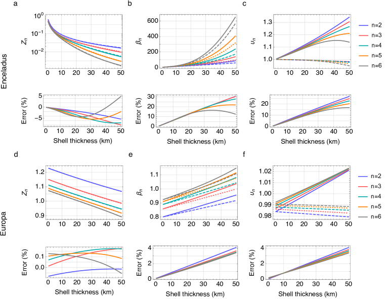
Figure 2: Admittance, $Z_{n}$, and momentum conservation equation terms $\beta_{n}$, and $\upsilon_{n}$ (Eq. (22)) as a function of shell thickness for different spherical harmonic degrees, $n$. Solid lines are thick shell solutions, dashed and dotted lines are thin shell approximation solutions (Beuthe, 2016), and bottom panels show the difference between the two solutions. We assume the interior structure parameters in Table 1 and a 1 km thick ocean for both Enceladus and Europa.

The convergence of the momentum conservation equation implies that ocean tidal heating solutions using the thick shell theory must also converge to the thin shell approximation solutions. We verify this by comparing the time- and surface-averaged tidal heating (Appendix C, Eqs. (77) and (79)) on Enceladus and Europa in Figs. 3 and 4. The difference between the thin and thick shell solutions can be large near resonant ocean thicknesses (discussed below). However, these resonances occur for oceans thinner than about 1 km, which is significantly smaller than the likely ocean thicknesses. For ocean thicknesses larger than 1 km, the thick shell solutions converge to the thin shell solutions as the shell thickness decreases, as expected. Assuming a 1 km thick shell for both Enceladus and Europa, the difference between the two solutions is less than 1% (Figs. 3 and 4).

Assuming a likely range of shell and ocean thicknesses for Europa and Enceladus, $h_{s}<25$ km and $h_{o}>10$ km, the accuracy of the thin shell approximation solutions is 3.5% and 4.1% for Europa (Fig. 3) and 3.2% and 26% for Enceladus (Fig. 4) for eccentricity tides and obliquity tides, respectively. The larger difference for obliquity forcing on Enceladus only occurs for small linear drag coefficients ($\alpha\lesssim 10^{-9}$ s^-1, Fig. 4f) and becomes similar to the difference for eccentricity forcing (3.2%) for larger linear drag coefficients (Fig. 4b, d).

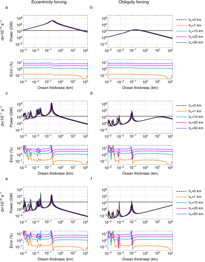
Figure 3: Ocean tidal heating power in Europa due to eccentricity and obliquity forcing as a function of ocean thickness for different shell thicknesses, $h_{s}$, and linear drag coefficients, $\alpha$. Solid lines are thick shell solutions, dotted lines are thin shell approximation solutions (Beuthe, 2016), and bottom panels show the difference between the two solutions. Dashed lines are surface ocean solutions without an overlying solid shell ($h_{s}=0$). The solid horizontal black line is the estimated radiogenic heating power (200 GW). We assume the interior structure parameters in Table 1.

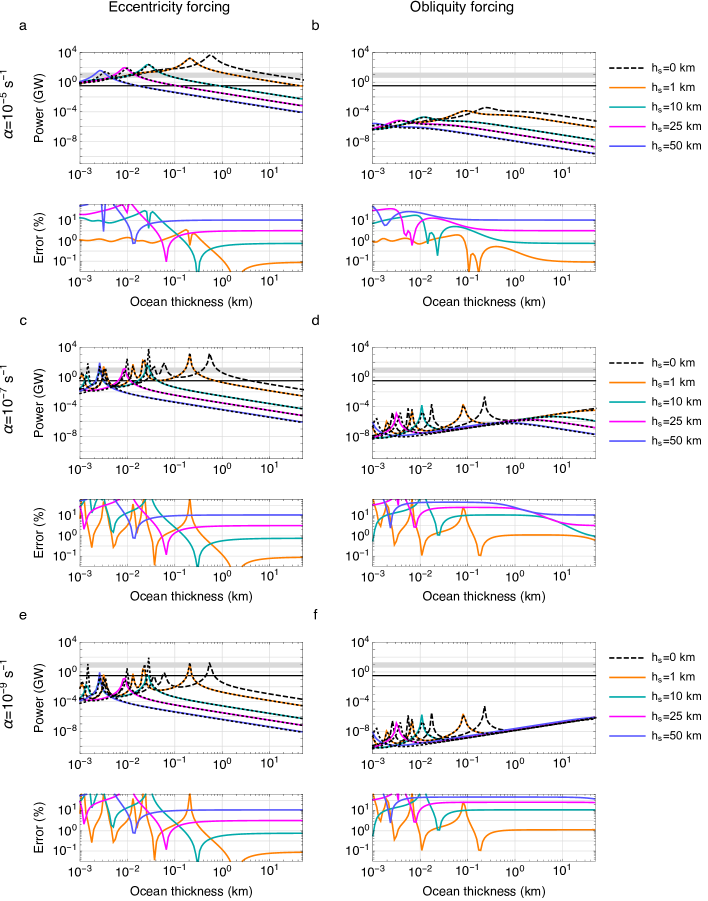
Figure 4: Ocean tidal heating power in Enceladus due to eccentricity and obliquity forcing as a function of ocean thickness for different shell thicknesses, $h_{s}$, and linear drag coefficients, $\alpha$. Solid lines are thick shell solutions, dotted lines are thin shell approximation solutions (Beuthe, 2016), and bottom panels show the difference between the two solutions. Dashed lines are surface ocean solutions without an overlying solid shell ($h_{s}=0$). The shaded gray region corresponds to the observational constraint of $3.9-18.9$ GW, and the solid horizontal black line is the estimated radiogenic heating power (0.3 GW). We assume the interior structure parameters in Table 1.

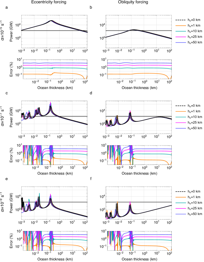
Figure 5: Europa’s ocean tidal heating power due to the obliquity and eccentricity forcing as a function of ocean thickness for different shell thicknesses, $h_{s}$, and linear drag coefficients, $\alpha$. Solid lines are thick shell solutions, dotted lines are rescaled surface ocean solutions (Eq. (26)), and bottom panels show the difference between the two solutions. Dashed lines are surface ocean solutions without an overlying solid shell ($h_{s}=0$). The solid horizontal black line is the estimated radiogenic heating power (200 GW). We assume the interior structure parameters in Table 1.

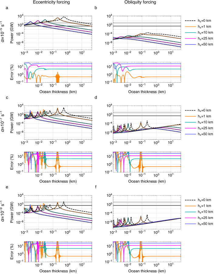
Figure 6: Enceladus’ ocean tidal heating power due to the obliquity and eccentricity forcing as a function of ocean thickness for different shell thicknesses, $h_{s}$, and linear drag coefficients, $\alpha$. Solid lines are thick shell solutions, dotted lines are rescaled surface ocean solutions (Eq. (26)), and bottom panels show the difference between the two solutions. Dashed lines are surface ocean solutions without an overlying solid shell ($h_{s}=0$). The shaded gray region corresponds to the observational constraint of $3.9-18.9$ GW, and the solid horizontal black line is the estimated radiogenic heating power (0.3 GW). We assume the interior structure parameters in Table 1.

2.4 Rescaling surface ocean solutions to subsurface ocean solutions

Assuming that the solutions to the LTE are dominated by spherical harmonic degree-two, it is possible to rescale surface ocean solutions to obtain subsurface ocean solutions (Beuthe, 2016). We can rescale the surface ocean solutions by a factor

$$\left(\frac{r_{t}}{R}\right)^{2}\left[\frac{(1-\xi_{2}\gamma_{2}^{L})}{\beta_{2}}\right]$$ (25)

in ocean thickness, and by a factor

$$\left(\frac{r_{t}}{R}\right)^{2}\left[\frac{(1-\xi_{2}\gamma_{2}^{L})}{\beta_{2}}\frac{\upsilon_{2}}{\gamma_{2}^{T}}\right]$$ (26)

in energy dissipation (C, Eqs. (77) and (79)), where $\gamma_{2}^{L}$ and $\gamma_{2}^{T}$ are given by Eq. (13) and $\upsilon_{2}$ and $\beta_{2}$ are given by Eq. (22). The first term in Eqs. (25) and (26) accounts for the change in Lamb’s parameter from $\text{$\epsilon$=}4\Omega^{2}R^{2}/(g(R)h_{o})$ for a surface ocean to $\epsilon=4\Omega^{2}r_{t}^{2}/(g(R)h_{o})$ for a subsurface ocean in our solutions based on the method of Longuet-Higgins (1968) (C). The second term accounts for the change in the momentum conservation equation terms from $1-\xi_{2}\gamma_{n}^{L}$ and $\gamma_{2}^{T}$ for a surface ocean (Eq. (12)) to $\upsilon_{n}$ and $\beta_{n}$ for a subsurface ocean (Eq. (21)). The resonant ocean thicknesses are independent of the forcing; therefore the scaling factor (25) for the ocean thickness does not include the scaling between the forcing terms ($\upsilon_{2}/\gamma_{2}^{T}$). Because the Love numbers in Eq. (13) for $\gamma_{2}^{L}$ and $\gamma_{2}^{T}$ are generally significantly smaller than unity for typical rigidities, these terms can be approximated as $\sim 1$.

Figs. 5 and 6 compare subsurface ocean solutions with rescaled surface ocean solutions for energy dissipation (C). The difference between the two solutions decreases with decreasing shell thickness, as expected. As in the thin shell approximation, the difference between the two solutions can be large near resonant ocean thicknesses (discussed below) but is small for the likely ocean thicknesses larger than about 1 km. Assuming the same likely range of shell and ocean thicknesses for Europa and Enceladus as above ($h_{s}<25$ km and $h_{o}>10$ km), the accuracy of the rescaled solutions is 2% for Europa (Fig. 5) and 13% for Enceladus (Fig. 6).

3 Time and surface-averaged tidal heating

Having illustrated the stabilizing effect of an overlying shell on equilibrium tides, we consider dynamic tides and the corresponding time- and surface-averaged ocean tidal heating in Figs. 3-6. We assume the three-layer interior structures for Enceladus and Europa described in Table 1 and consider a range of shell and ocean thicknesses. Given a velocity solution of the Laplace tidal equation, the dissipated energy per unit time and surface area can be found with Eq. (6), and the time- and surface-averaged energy dissipation can be found by integrating this equation (C, Eq. (77). Energy conservation requires that the time- and surface-averaged dissipated energy and work done by the tide must be equal, which provides an alternative expression (C, Eq. (79).

Tidal heating decreases with shell thickness, as expected due to the stabilizing effect of an overlying shell. This effect is more pronounced on Enceladus than on Europa (e.g. compare Figs 3 and 4) because the effective rigidity on a small body like Enceladus is larger (B.2). This difference can also be seen in the Love numbers. The magnitude of the Love numbers decreases rapidly with shell thickness for Enceladus while it remains relatively constant for Europa (A). A 1 km thick shell can reduce tidal heating by about an order of magnitude for Enceladus, and by tens of percent for Europa, compared with tidal heating solutions without an overlying shell.

As previously shown for surface oceans (Tyler, 2008, 2009, 2011; Matsuyama, 2014), tidal heating can increase sharply for ocean thicknesses for which the tidal flow is resonantly enhanced (the sharp peaks in Figs. 3 and 4). Eccentricity and obliquity forcing can generate gravity wave resonances for oceans thinner than about 1 km, limiting their impact because the oceans in Enceladus and Europa are likely significantly thicker. Obliquity forcing can also generate Rossby-Haurwitz waves (Tyler, 2008), and this produces a tidal heating increase with ocean thickness for small linear drag coefficients (Figs. 3f and 4f). In addition to reducing the magnitude of tidal heating, increasing the shell thickness also decreases the resonant ocean thicknesses, as illustrated by Beuthe (2016) using a thin shell approximation.

Enceladus’ total endogenic power radiated from the south polar terrain (SPT) has been estimated to be $15.8\pm 3.1$ GW based on Cassini infrared emission observations (Howett et al., 2011). The actual uncertainty is likely larger due to the difficulty of estimating and subtracting the thermal emission associated with absorbed solar radiation (Spencer et al., 2013). This may explain the difference from the previous estimate of $5.8\pm 1.9$ GW (Spencer et al., 2006). We adopt a range of $3.9-18.9$ GW as a conservative constraint that includes all available estimates. For the range of likely shell and ocean thicknesses inferred from gravity and topography constraints, $h_{s}=23\pm 4$ km and $h_{o}=38\pm 4$ km (Beuthe et al., 2016), the total power is lower than the observed value (Fig. 4). Ocean tidal heating driven by eccentricity forcing can match the observed value; however, this requires ocean and shell thicknesses that are significantly smaller than the values inferred from gravity and topography constraints (Fig. 4). Additionally, a more direct comparison with the observed value requires computing the power dissipated beneath SPT alone, which would worsen the discrepancy.

The radiogenic heating power is about 200 GW and 0.3 GW for Europa and Enceladus respectively assuming the fiducial values in Table 1 and a present-day, chondritic radiogenic heating rate of $4.5\times 10^{-12}$ W kg^-1 for the core (Spohn and Schubert, 2003). For Europa, ocean tidal heating is comparable to radiogenic heating for eccentricity forcing, $\alpha\gtrsim 10^{-5}$ s^-1, and ocean thicknesses $\lesssim 50$ km (Fig. 3a); or obliquity forcing, $\alpha\lesssim 10^{-7}$ s^-1, and ocean thicknesses $\sim 25$ km (Fig. 3d, f). For Enceladus, ocean tidal heating is comparable to radiogenic heating for eccentricity forcing and $\alpha\gtrsim 10^{-5}$ s^-1 (Fig. 4a); however, this requires ocean and shell thicknesses that are significantly smaller than the values inferred from gravity and topography constraints; and ocean tidal heating due to obliquity forcing is generally smaller than that due to eccentricity forcing due to Enceladus’ small obliquity (compare the left and right panels in Fig. 4). It is worth noting that ocean tidal heating may be generally weaker than solid-body tidal heating (Chen et al., 2014; Beuthe, 2016); however, the effect of ocean dynamics remains important because ocean tides can increase solid-body tidal heating.

4 Temporal and surface distribution of tidal heating and tides

Thus far we have focused on the time- and surface-averaged ocean tidal heating. While this is important for the global average tidal heating and has implications for the long-term thermal, rotational, and orbital evolution, the temporal and surface distribution of ocean tidal heating contains unique features that may be observable, as shown in sections 4.1 and 4.2.

4.1 Surface distribution of ocean tidal heating

Figs. 7 and 8 show the surface distribution of the tidal heating flux (Eq. (6)) averaged over the tidal forcing period. We assume the Enceladus and Europa model parameters in Table 1.

For Enceladus, we assume the likely shell and ocean thicknesses inferred from gravity and topography constraints for Enceladus, $h_{s}=23$ km and $h_{o}=38$ km (Beuthe et al., 2016). For Europa, we assume values that are consistent with the constraint of a combined ocean and shell thickness between 80 and 170 km (Anderson et al., 1998), $h_{s}=10$ km and $h_{o}=100$ km. The surface distribution of the time-averaged tidal heating flux is similar to that of surface oceans (compare Figs. 7 and 8 with Fig. 7 of Chen et al., 2014) for small linear drag coefficients ($\alpha\lesssim 10^{-7}$ s^-1).

Tidal heating in a subsurface ocean can generate horizontal shell thickness variations if the shell is not convective (Ojakangas and Stevenson, 1986; Ojakangas, 1989b; Nimmo et al., 2007; Nimmo and Bills, 2010). The surface distribution of the time-averaged tidal heating flux is distinct from that due solid dissipation in the shell (Ojakangas, 1989b; Tobie et al., 2005; Beuthe, 2013), with higher dissipation near the equator and poles for eccentricity and obliquity forcing respectively (Figs. 7 and 8). Therefore, observations of these variations can be used to constrain ocean tidal heating. The tidal heating flux is orders of magnitude larger for Europa than for Enceladus (compare Figs. 7 and 8) due to Enceladus’ larger effective rigidity (B.2) and small obliquity, which has implications for observable horizontal shell thickness variations.

The surface heat flux due to radiogenic heating is about $7\times 10^{-3}$ W m^-2 and $4\times 10^{-4}$ W m^-2 for Europa and Enceladus respectively assuming the fiducial values described above and a present-day, chondritic radiogenic heating rate of $4.5\times 10^{-12}$ W kg^-1 for the core (Spohn and Schubert, 2003). As discussed above for the time- and surface-averaged tidal heating results, ocean tidal heating in Europa is comparable to radiogenic heating for eccentricity forcing and $\alpha\gtrsim 10^{-5}$ s^-1 (Fig. 7a) or obliquity forcing and $\alpha\lesssim 10^{-7}$ s^-1 (Fig. 7f, h). Ocean tidal heating in Enceladus is significantly weaker than radiogenic heating (Fig. 8).

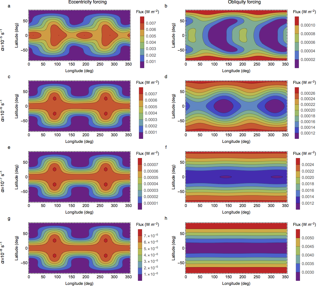
Figure 7: Europa’s surface distribution of ocean tidal heating due to eccentricity and obliquity forcing for different linear drag coefficients, $\alpha$. Contours show the energy flux averaged over the tidal forcing period. We assume the parameters in Table 1.

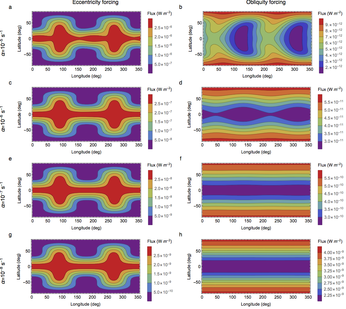
Figure 8: Enceladus’ surface distribution of ocean tidal heating due to eccentricity and obliquity forcing for different linear drag coefficients, $\alpha$. Contours show the energy flux averaged over the tidal forcing period. We assume the parameters in Table 1.

4.2 Surface displacement phase lag and amplitude

The surface displacements driven by eccentricity and obliquity forcing can have phase lags relative to the forcing tidal potential due to the delayed ocean response. To compute this phase lag, we compare the dynamic and equilibrium surface displacements $\eta^{R}$ (Eq. (15)). The former is the solution of the LTE coupled to a thick shell, while the latter assumes that the satellite deforms instantaneously in response to the forcing tidal potential and can be computed by ignoring the pressure potential term, $U_{nm}^{P}$, in Eq. (15).

Figs. 9 and 10 and show the surface displacement phase lag and amplitude for Europa and Enceladus. We compute the surface displacement time lag $\delta t$ and corresponding phase lag $\delta\phi=\Omega\delta t$ by finding the wave maximum using Eq. (15). We assume the model parameters in Table 1 and consider a wide range of ocean and shell thicknesses and linear drag coefficients. Eccentricity forcing generally produces greater tidal amplitudes due to the large eccentricity values relative to the obliquity values. Despite the small obliquity values, obliquity forcing generally produces larger phase lags due to the generation of Rossby-Haurwitz waves.

The amplitudes of the equilibrium and dynamic surface displacement are comparable, and the latter scales linearly with the forcing tidal potential, which in turn scales linearly with eccentricity, $e$, and obliquity, $\theta_{0}$ (Eq. 5). Assuming the minimum energy Cassini state values in Table 1, $e/\theta_{0}\sim 10$ and $e/\theta_{0}\sim 10^{3}$ for Europa and Enceladus respectively (note that the obliquities in the forcing potential must be in radians), which is consistent with the differences in the obliquity and eccentricity surface displacement amplitudes in Figs. 9 and 10. The surface displacement amplitude increases with decreasing shell thickness, as expected due to the weaker resistance to deformation.

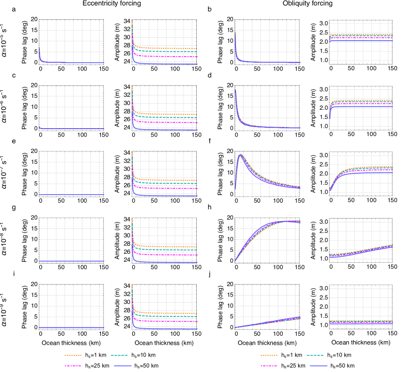
Figure 9: Surface displacement phase lag and amplitude due to eccentricity and obliquity forcing on Europa as a function of ocean thickness for different shell thicknesses and linear drag coefficients. The phase lag and amplitude are computed at 0^∘ and $45^{\circ}$ latitudes for eccentricity and obliquity forcings respectively, where the amplitude is maximum. The phase lag is given by $\delta\phi=\Omega\delta t$, where $\Omega$ is the rotation rate and $\delta t$ is the time lag. We assume the interior structure parameters in Table 1.

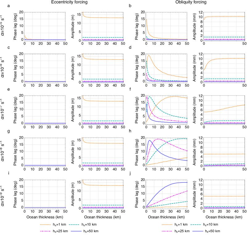
Figure 10: Surface displacement phase lag and amplitude due to eccentricity and obliquity forcing on Enceladus as a function of ocean thickness for different shell thicknesses and linear drag coefficients. The phase lag and amplitude are computed at 0^∘ and $45^{\circ}$ latitudes for eccentricity and obliquity forcings respectively, where the amplitude is maximum. The phase lag is given by $\delta\phi=\Omega\delta t$, where $\Omega$ is the rotation rate and $\delta t$ is the time lag. We assume the interior structure parameters in Table 1.

In the absence of Rossby-Haurwitz waves, the surface displacement phase lag decreases with increasing ocean thickness (Figs. 9 and 10, eccentricity tide results). In this case, dynamic effects decrease as the ocean thickness increases away from the resonant thicknesses, decreasing the phase lag because the tide response becomes more static. We also verify this for obliquity forcing by removing the westward component of the obliquity forcing tidal potential (Eq. 5), which prevents the generation of Rossby-Haurwitz waves. The generation of Rossby-Haurwitz waves by obliquity forcing produces phase lags that are larger than those produced by eccentricity forcing, and introduces a complex dependence of the phase lag on ocean thickness (Figs. 9 and 10). For Enceladus, the phase lag is also sensitive to the overlying shell thickness (Fig. 10).

Fig. 9 shows the amplitude and phase lag of the surface displacement on Europa. Assuming the fiducial shell and ocean thicknesses ($h_{s}=10$ km and $h_{o}=100$ km) and linear drag coefficients $\alpha<10^{-5}$ s^-1, the amplitude and phase lag are 26.5 m and $<1$ degree for eccentricity forcing, and $<2.5$ m and $<18$ degrees for obliquity forcing. The larger obliquity phase lags correspond to linear drag coefficients $\lesssim 10^{-7}$ s^-1 and smaller amplitudes (e.g. $5$ degrees and 2.5 m for $\alpha=10^{-7}$ s^-1, and $18$ degrees and 1.6 m for $\alpha=10^{-8}$ s^-1), and measurement of this lag (e.g. by Europa Clipper) would provide a probe of ocean thickness. Ignoring the dynamic ocean response, there can be a phase lag due to the viscoelastic behavior of the shell. This phase lag is smaller than 2 degrees for shell thicknesses smaller than 100 km (Moore and Schubert, 2000); therefore, the phase lag due to the delayed ocean response can be significantly larger for this range of shell thicknesses.

Fig. 10 shows the amplitude and phase lag of the surface displacement on Enceladus. Assuming the fiducial shell and ocean thicknesses ($h_{s}=23$ km and $h_{o}=38$ km) and linear drag coefficients $\alpha<10^{-5}s^{-1}$, the amplitude and phase lag are 0.8 m and $<1$ degrees for eccentricity forcing, and $<0.6$ mm and $<13$ degrees for obliquity forcing. The amplitude increases rapidly with decreasing shell thickness (e.g. 13.2 m and $<11$ mm for eccentricity and obliquity forcing respectively assuming a shell thickness of 1 km and $\alpha=10^{-5}$ s^-1) due to Enceladus’ small size and large effective rigidity (Appendix B.2). As discussed above, the phase lag dependence on the ocean and shell thicknesses is complex due to the generation of Rossby-Haurwitz waves. The large phase lags driven by obliquity forcing may have implications for the observed phase lag of about 50 degrees (time delay of about 5 hours) in plume activity with respect to predictions based on tidal stress models (Hedman et al., 2013; Nimmo et al., 2014). However, obliquity forcing can only produce surface displacement amplitudes of the order of mm, generating stresses that are negligible. Furthermore, all modeling so far has assumed that eccentricity forcing is the source of tidal modulation (Hedman et al., 2013; Nimmo et al., 2014), and the predicted phase lag due to eccentricity forcing is smaller than 2.7 degrees for shells thicknesses larger than 1 km.

5 Discussion

We consider tidal heating in the subsurface oceans of Enceladus and Europa using a new theoretical treatment that is applicable to icy satellites with thin oceans overlaid by incompressible elastic shells of arbitrary thickness.

The shell’s resistance to dynamic ocean tides reduces ocean tidal heating, and this effect is larger on Enceladus than on Europa due to the Enceladus’ small size and larger effective rigidity (Appendix B.2). Tidal heating driven by eccentricity forcing is generally dominant over that driven by obliquity forcing, with the exception of Europa models with ocean thicknesses $\gtrsim 10$ km and linear drag coefficient $\alpha\lesssim 10^{-7}$ s^-1 (Fig. 3), and Enceladus models with ocean and shell thicknesses $\gtrsim 10$ km and linear drag coefficients $\alpha\lesssim 10^{-9}$ s^-1 (Fig. 4).

We assume a conductive shell that is entirely elastic. For a convecting shell, only the near-surface part is likely to be rigid, reducing the rigid shell thickness and its resistance to tides. This increases energy dissipation in the shell and ocean. Applying the thin shell approximation of Beuthe (2016) to Enceladus and assuming the likely range of shell and ocean thicknesses, convection in the shell increases energy dissipation in the shell and ocean by about an order of magnitude and tens of percent, respectively (Beuthe, 2016, Figs. 13 and 14). The larger effect on shell energy dissipation arises because a convective shell is more dissipative than a conductive one (Beuthe, 2016, Eqs. (101) and (102)). Our assumed shear modulus of 3.5 GPa is uncertain and may be lower due to fractures or periodic tidal forcing (Wahr et al., 2006). This has not been observed in laboratory experiments; however, only a limited range of temperatures and forcing frequencies that are significantly higher than those in icy satellites is accessible (Hammond et al., 2018). The deformation of the shell is sensitive to both it thickness and shear modulus, and decreases with the product of these two quantities (Wahr et al., 2006; Beuthe, 2015b, a). Thus, reducing the shear modulus has a similar effect as reducing the thickness, and the wide range of shell thicknesses considered in this paper can also be interpreted as a wide range of possible shear moduli.

The time-averaged surface distribution of ocean tidal heating (Figs. 7 and 8) is distinct from that due to dissipation in the solid shell, with higher dissipation near the equator and poles for eccentricity and obliquity forcing respectively (Figs. 7 and 8). This can lead to unique horizontal shell thickness variations if the shell is conductive, providing constraints on ocean tidal heating. Characterizing the expected horizontal shell thickness variations requires solving the coupled thermal-orbital evolution, and previous studies have investigated various aspects of this coupled problem (e.g. Ojakangas and Stevenson, 1986; Ross and Schubert, 1990; Fischer and Spohn, 1990; Showman et al., 1997; Hussmann and Spohn, 2004; Běhounková et al., 2012). However, these studies ignore ocean tidal heating and assume that energy dissipation occurs only in solid regions. Chen and Nimmo (2016) investigated the role of tidal heating in a surface magma ocean on the early evolution of the Earth-Moon system. Our thick shell theory can be coupled to thermal and orbital evolution models to study the effect of tidal heating in subsurface oceans.

The surface displacement driven by eccentricity and obliquity forcing can have a phase lag relative to the forcing tidal potential due to the delayed ocean response. For Europa and Enceladus, eccentricity forcing generally produces greater tidal amplitudes due to the large eccentricity values relative to the obliquity values. Despite the small obliquity values, obliquity forcing generally produces larger phase lags due to the generation of Rossby-Haurwitz waves. Figs. 9 and 10 summarize the surface displacement results for Europa and Enceladus. The phase lag due to the delayed ocean response can be significantly larger than the phase lag due to the viscoelastic behavior of the shell (e.g. Moore and Schubert, 2000; Kamata et al., 2016). Ignoring the horizontal ocean dynamics, a small phase lag (less than about 10 degrees) can be used as a proxy for the presence of a subsurface ocean in Ganymede (Kamata et al., 2016). Given our result that large phase lags can be generated by obliquity forcing on Europa and the similar Cassini state obliquities of Ganymede and Europa (Bills, 2005), future Ganymede studies should consider the horizontal ocean dynamics captured by the LTE. Although eccentricity tides likely dominate obliquity tides at Europa, the expected obliquity tide amplitude (about 2.5 m) and phase lag (up to 18 degrees) are potentially detectable by a future spacecraft mission such as Europa Clipper. Measuring this effect would help determine the ocean thickness and effective drag coefficient.

For the range of likely shell and ocean thicknesses, the thin shell approximation of Beuthe (2016) is generally accurate to less than about 4% for Enceladus and Europa (Figs. 3 and 4), with the exception of obliquity forcing on Enceladus and small linear drag coefficients ($\alpha\lesssim 10^{-9}$ s^-1) for which the accuracy is less than 26% (Fig. 4f). It is worth noting that the thick shell theory described in this paper is general enough to be applicable to any interior rheology. The effect of compressibility can be taken into account by using compressible Love numbers instead of incompressible ones (e.g. Tobie et al., 2005; Wahr et al., 2009; Kamata et al., 2015) and is likely small. For example, the assumption of an incompressible shell introduces errors of about 8% for the radial tidal displacements on Enceladus (Beuthe, 2018, Fig. 1). The viscoelastic response can be derived from the elastic response using the correspondence principle (Peltier, 1974) in the Laplace (e.g. Jara-Orué and Vermeersen, 2011) or Fourier (e.g. Moore and Schubert, 2000; Tobie et al., 2005; Wahr et al., 2009; Kamata et al., 2015) domains. The effect of taking into account viscoelasticity is also likely small. For example, the radial tidal displacement on Europa increases by about 5% when viscoelasticity is taken into account (Wahr et al., 2009, Fig. 1, solid line). The elastic limit results of this paper provide an upper estimate of the shell effect on ocean tidal heating. The thin shell approximation of Beuthe (2016) provides an explicit treatment of viscoelasticity and compressibility of the crust in terms of the effective shear modulus and Poisson’s ratio (Beuthe, 2016, Eq. (B.4)). More importantly, the dynamic ocean tides are described by a modified Laplace tidal equation that assumes a thin homogeneous ocean. This approximation is likely reasonable for Europa if the combined ocean and shell thickness is smaller than about 170 km (Anderson et al., 1998). However, it may introduce significant errors for Enceladus if the ocean thickness is $38\pm 4$ km (Beuthe et al., 2016). The assumption of a uniform thickness for the shell and ocean may also introduce errors given the likely variations in these parameters (McKinnon, 2015; Thomas et al., 2016; Beuthe et al., 2016; Beuthe, 2018).

We assume the simplest linear drag formalism to model dissipation. Earth’s ocean tidal heating studies commonly assume a quadratic bottom drag formalism based on the assumption that drag arises due to turbulent flow interacting with a bottom boundary. We use an order-of-magnitude analysis (Eq. 7) to estimate a linear drag coefficient from the nominal bottom drag coefficient $c_{D}\sim(2-3)\times 10^{-3}$ assumed in Earth (Lambeck, 1980; Jayne and St Laurent, 2001; Egbert and Ray, 2001; Green and Nycander, 2013), Titan (Sagan and Dermott, 1982), and Jovian planets (Goldreich and Soter, 1966) studies. The numerical method of Hay and Matsuyama (2017) can solve the LTE with the bottom drag formalism, and our thick shell theory can be used to extend this method to include the effect of an overlying solid shell.

Appendix

Appendix A Love numbers

A.1 Propagator matrix method

We compute the tidal, load, and pressure Love numbers using the propagator matrix method (e.g. Sabadini and Vermeersen, 2004). Following the notation of Sabadini and Vermeersen (2004), the spheroidal solution vector containing the spherical harmonic expansion coefficients is

$$\mathbf{y}_{nm}=(U_{\ell m},\>V_{\ell m},\,R_{\ell m},\,S_{\ell m},\,-\Phi_{nm},\>Q_{nm}),$$ (27)

where $U_{nm}$ and $V_{nm}$ are the radial and tangential displacements, $R_{\ell m}$ and $S_{\ell m}$ are the radial and tangential stress, $\Phi_{nm}$ is the gravitational potential, and $Q_{nm}$ is the potential stress. Hereafter, we drop the “n” and “m” subscripts to simplify the notation.

The surface boundary conditions for the radial, tangential, and potential stresses are (Sabadini and Vermeersen, 2004; Beuthe, 2016):

$$\mathbf{b}=(y_{3}(R),\,y_{4}(R),\,y_{6}(R))=\begin{cases}\left(0,\,0,\,-\frac{2n+1}{R}\right)U^{T}(R)&\mbox{tidal}\\ \left(-\frac{2n+1}{3}\bar{\rho},\,0,\,-\frac{2n+1}{R}\right)U^{L}(R)&\mbox{surface loading}\\ \left(\bar{\rho},\,0,\,0\right)U^{P}(R)&\mbox{surface pressure,}\end{cases}$$ (28)

where $U^{T}(R)$, $U^{L}(R)$, and $U^{P}(R)$ are the tidal, surface loading, and surface pressure loading potentials. In this equation, $R$ and $\bar{\rho}$ are the mean radius and density respectively, and the subscript in the solution vector now refers to the third, fourth, and sixth components of the solution vector. Eq. (28) is equivalent to Eqs. (C.5), (C.6), and (E.3) of Beuthe (2016) if we take into account the following differences. First, we use the convention of Sabadini and Vermeersen (2004) for the solution vector (Eq. (27)), while Beuthe (2016) uses the convention of Takeuchi and Saito (1972). The two conventions differ by exchanging the definitions of $y_{2}$ and $y_{3}$ and by changing the sign of both $y_{5}$ and $y_{6}$. Second, we normalize the pressure potential as $y_{3}(R)=\bar{\rho}U^{P}(R)$, whereas Beuthe (2016) normalizes it as the pressure part of a load potential, $y_{3}(R)=-(2n+1)\bar{\rho}U^{P}(R)/3$. Our sign convention implies that a positive pressure potential leads to a positive radial displacement, whereas the sign convention of Beuthe (2016) implies that a positive pressure potential leads to a negative radial displacement (as in the case of a mass load).

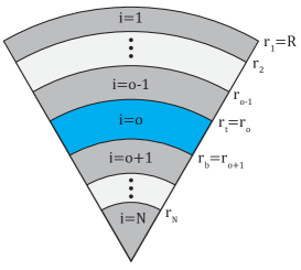
Figure 11: Definition of the nomenclature used to describe the internal layers of a satellite. Layers with $1\leq i<o-1$ are the shell overlying the ocean, the layer with $i=0$ is he ocean, layers with $o<i\leq N$ are the layers below the ocean, and the layer with $i=N$ is the core.

The solution vector at the core is

$$\mathbf{y}^{(N)}(r_{N})=\mathbf{I}_{c}\text{{C}}_{c},$$ (29)

where $r_{N}$ is the core radius (Fig. 11), the $(N)$ superscript indicates the solution vector corresponds to that of the core layer, $\mathbf{I}_{c}$ is given by Eq. (1.103) of Sabadini and Vermeersen (2004) for a liquid core, and $\mathbf{C}_{c}$ is a constant vector. For an incompressible solid core, $\mathbf{I_{c}}$ is given by the first three columns of the matrix in Eq. (1.74) of Sabadini and Vermeersen (2004). Propagating the solution vector from the core to the surface, the solution vector at the surface is

$$\mathbf{y}^{(1)}(R)=\left(\prod_{i=1}^{N-1}\mathbf{Y}^{(i)}(r_{i})\mathbf{Y}^{(i)^{-1}}(r_{i+1})\right)\mathbf{I}_{c}\text{{C}}_{c},$$ (30)

where the fundamental matrices $\mathbf{Y}^{(i)}$ and $\mathbf{Y}^{(i)^{-1}}$ are given by Eqs. (1.74) and (1.75) of Sabadini and Vermeersen (2004) assuming incompressible layers. Once again, we drop the spherical harmonic subscript (“n” in this work, “$\ell$” in Sabadini and Vermeersen (2004)) to simplify the notation. The superscript “$i$” indicates that the properties (e.g., density, gravity, shear modulus) of the layer $i$ must be used (Fig. 11). There is a typographical error in the sign of third component in Eq. (1.76) of Sabadini and Vermeersen (2004), this equation should read

$$\text{diag}(\mathbf{D}(r))=\frac{1}{2n+1}\left((n+1)r^{-n-1},\,\frac{n(n+1)}{2(2n-1)}r^{-n+1},\,r^{-n+1},\,nr^{n},\,\frac{n(n+1)}{2(2n+3)}r^{n+2},\,-r^{n+1}\right).$$

Using the boundary conditions at the surface,

$$\mathbf{P}_{1}\left(\prod_{i=1}^{N-1}\mathbf{Y}^{(i)}(r_{i})\mathbf{Y}^{(i)^{-1}}(r_{i+1})\right)\mathbf{I}_{c}\text{{C}}_{c}=\mathbf{b},$$ (31)

where

$$\mathbf{P_{1}}\equiv\left(\begin{array}[]{cccccc}0&0&1&0&0&0\\ 0&0&0&1&0&0\\ 0&0&0&0&0&1\end{array}\right)$$ (32)

is a projection matrix for the third, fourth, and sixth components of the solution vector. Thus,

$$\mathbf{C}_{c}=\left[\mathbf{P}_{1}\left(\prod_{i=1}^{N-1}\mathbf{Y}^{(i)}(r_{i})\mathbf{Y}^{(i)^{-1}}(r_{i+1})\right)\mathbf{I}_{c}\right]^{-1}\mathbf{b},$$ (33)

and the solution vector at the surface can be written as

$$\mathbf{y}^{(1)}(R)=\left(\prod_{i=1}^{N-1}\mathbf{Y}^{(i)}(r_{i})\mathbf{Y}^{(i)^{-1}}(r_{i+1})\right)\mathbf{I}_{c}\left[\mathbf{P}_{1}\left(\prod_{i=1}^{N-1}\mathbf{Y}^{(i)}(r_{i})\mathbf{Y}^{(i)^{-1}}(r_{i+1})\right)\mathbf{I}_{c}\right]^{-1}\mathbf{b}.$$ (34)

Using the boundary conditions in Eq. (28), the tidal and loading Love numbers at the satellite surface are

$$k(R) =-y_{5}^{(1)}(R)-1$$

$$h(R) =g(R)y_{1}^{(1)}(R)$$

$$\ell(R) =g(R)y_{2}^{(1)}(R).$$ (35)

The pressure Love numbers are also defined by this equation, except $k^{P}(R)=-y_{5}^{(1)}(R)$ because pressure forcing can only produce an induced gravitational potential.

A.2 Propagator matrix method with internal liquid layers

The presence of an internal liquid layer requires a special treatment because this causes the layers above and below the liquid layer to be mechanically decoupled while remaining gravitationally coupled. We use the method of Jara-Orué and Vermeersen (2011) to extend the propagator matrix method to take into account the mechanical decoupling. In this case,

$$\left(\begin{array}[]{c}y_{1}^{(1)}(R)\\ y_{2}^{(1)}(R)\\ y_{5}^{(1)}(R)\end{array}\right)\equiv\left(\begin{array}[]{c}U(R)\\ V(R)\\ -\Phi(R)\end{array}\right)=\mathbf{P_{35}}\mathbf{W}_{2}(\mathbf{W}_{1})^{-1}\mathbf{b},$$ (36)

where $\mathbf{P}_{35}$, $\mathbf{W}_{2}$, $\mathbf{W}_{1}$, and $\mathbf{b}$ are defined by Eqs. (A.18), (A.19), (A.21)-(A.23), and (B.20) of Jara-Orué and Vermeersen (2011). The solution vector at the ocean top $(r_{o})$ can be found by propagating the surface solution to the ocean top,

$$\mathbf{y}^{(o-1)}(r_{o})=\left[\prod_{i=1}^{o-1}\mathbf{Y}^{(i)}(r_{i})\mathbf{Y}^{(i)^{-1}}(r_{i+1})\right]^{-1}\mathbf{y}^{(1)}(R),$$ (37)

where

$$\mathbf{y}^{(1)}(R)=\begin{cases}\left(U(R),\,V(R),\,0,\,0,\,-\Phi(R),\,-\frac{2n+1}{R}\right)U^{T}(R)&\mbox{tidal}\\ \left(U(R),\,V(R),\,-\frac{2n+1}{3}\bar{\rho},\,0,\,-\Phi(R),\,-\frac{2n+1}{R}\right)U^{L}(R)&\mbox{surface loading}\\ \left(U(R),\,V(R),\,\bar{\rho},\,0,\,-\Phi(R),\,0\right)U^{P}(R)&\mbox{surface pressure,}\end{cases}$$ (38)

where $U^{T}$, $U^{L}$, and $U^{P}$ are the tidal, surface loading, and surface pressure loading potentials. The sign convention for pressure forcing implies that a positive pressure potential leads to a positive radial displacement. As described above for the case without internal liquid layers, we drop the spherical harmonic subscript (“n” in this work, “$\ell$” in Jara-Orué and Vermeersen (2011)) to simplify the notation.

The solution vector at the ocean bottom ($r=r_{b}$, Fig. 11) can be found using the $\mathbf{C}_{icy}$ vector containing constant terms (Jara-Orué and Vermeersen, 2011, Eq. A.20) to obtain the 3-component constant vector $\mathbf{C}_{c}$ for the solution vector at the core:

$$\mathbf{C}_{icy}\equiv(K_{4},\,K_{5},\,K_{1},\,K_{2},\,K_{3})=(\mathbf{W}_{1})^{-1}\mathbf{b},$$ (39)

$$\mathbf{C}_{c}\equiv(K_{1},\,K_{2},\,K_{3}),$$ (40)

and

$$\mathbf{y}^{(o+1)}(r_{b})=\left(\prod_{i=o+1}^{N-1}\mathbf{Y}^{(i)}(r_{i})\mathbf{Y}^{(i)^{-1}}(r_{i+1})\right)\mathbf{I_{c}C_{c}}.$$ (41)

For a single core layer beneath the ocean, $\mathbf{y}^{(o+1)}(r_{b})=\mathbf{I_{c}C_{c}}$.

Using the boundary conditions in Eq. (28), the tidal and loading Love numbers are

$$k(r) =-y_{5}^{(i)}(r)-(r/R)^{n}$$

$$h(r) =g(R)y_{1}^{(i)}(r)$$

$$\ell(r) =g(R)y_{2}^{(i)}(r),$$ (42)

where $i=1$ and $r=R$ for the surface, $i=o-1$ and $r=r_{t}$ for the ocean top, and $i=o+1$ and $r=r_{b}$ for the ocean bottom (Fig. 11). Once again, the pressure Love numbers are also defined by this equation, except $k(r)=-y_{5}^{(i)}(r)$ because pressure forcing can only produce an induced gravitational potential.

A.3 Interior pressure forcing in a subsurface ocean

As discussed in the main text, we introduce pressure Love numbers to describe the dynamic pressure forcing in the ocean and couple the LTE with the Love number equations (the mass and momentum conservation equations and Poisson’s equation). Computing the Love numbers due to interior pressure forcing in a subsurface ocean requires further modifications to the method of Jara-Orué and Vermeersen (2011).

Dynamic pressure forcing in the ocean changes the boundary conditions at the ocean top and bottom. For pressure forcing at the ocean top ($r=r_{t}$), the third component of Eqs (A.12) in Jara-Orué and Vermeersen (2011) becomes

$$\sigma_{rr}^{(o-1)}(r_{t})=\rho_{o}g(r_{t})K_{4}-\rho_{o}U^{P}(r_{t}),$$ (43)

where $i=o-1$ corresponds to the layer overlying the ocean (Fig. 11). For pressure forcing at the ocean bottom ($r=r_{b}$), the third component of Eqs (A.14) in Jara-Orué and Vermeersen (2011) becomes

$$\sigma_{rr}^{(o+1)}(r_{b})=-\rho_{o}g(r_{t})K_{6}+\rho_{o}U^{P}(r_{b}),$$ (44)

where $i=o+1$ corresponds to the layer below the ocean (Fig. 11). The sign convention for the pressure load $U^{P}$ implies that a positive pressure potential leads to a positive radial displacement. In the thin ocean limit,

$$U^{P}(r_{b})=-U^{P}(r_{t}),$$ (45)

and Eqs. (43) and (44) can be written as a function of a single forcing term evaluated at the ocean top or bottom. This allow us to describe ocean pressure forcing in terms of a single Love number evaluated at the ocean top or bottom instead of the traditional approach describing each forcing with a different Love number, as described below.

A.3.1 Interior pressure forcing at the ocean top

Dynamic pressure forcing at the ocean top can be taken into account by modifying the boundary condition in Eq. (A.20) of Jara-Orué and Vermeersen (2011),

$$\mathbf{b}+\mathbf{b}^{t}=W_{1}C_{icy},$$ (46)

where $\mathbf{b}=(y_{3}(R),\,y_{4}(R),\,y_{6}(R))=(0,\,0,\,0)$ for interior pressure forcing and

$$\mathbf{b^{t}=}\rho_{o}U^{P}(r_{t})\left(0,\,0,\,B_{33}^{si},\,B_{43}^{si},\,B_{63}^{si}\right).$$ (47)

With this modified boundary condition, the constants vector $C_{icy}=(K_{4},\,K_{5},\,K_{1},\,K_{2},\,K_{3})=W_{1}^{-1}(\mathbf{b}+\mathbf{b}^{t})$, the core constants vector $C_{c}\equiv(K_{1},\,K_{2},\,K_{3})$.

The unconstrained solution at the surface (Eq. (B.19) of Jara-Orué and Vermeersen (2011)) becomes

$$\mathbf{X}=P_{35}W_{2}C_{icy}-\rho_{o}U^{P}(r_{t})\left(\begin{array}[]{c}B_{13}^{si}\\ B_{23}^{si}\\ B_{53}^{si}\end{array}\right),$$ (48)

where the ice shell propagation matrix is

$$\mathbf{B}^{si}=\prod_{i=1}^{o-1}\mathbf{Y}^{(i)}(r_{i})\mathbf{Y}^{(i)^{-1}}(r_{i+1}).$$ (49)

The solution vector at the surface is given by $\mathbf{y}^{(1)}(R)=(X_{1},\,X_{2},\,0,\,0,\,X_{3},\,0)$, the solution vector at the ocean top, $\mathbf{y}^{(o-1)}(r_{t})$, can be obtained by propagating the surface solution through the shell (Eq. (37)), and the solution vector at the ocean bottom is given by Eq. (41) or $\mathbf{y}^{(o+1)}(r_{o+1})=\mathbf{I_{c}C_{c}}$ for a single core layer beneath the ocean.

Given the solution vector at a radius $r$, the corresponding Love numbers are given by Eq. (42), except $k(r)=-y_{5}^{(i)}(r)$ because pressure forcing can only produce an induced gravitational potential.

A.3.2 Interior pressure forcing at the ocean bottom

Dynamic pressure forcing at the ocean top can be taken into account by modifying the boundary condition in Eq. (A.20) of Jara-Orué and Vermeersen (2011),

$$\mathbf{b}+\mathbf{b}^{b}=W_{1}C_{icy},$$ (50)

where $\mathbf{b}=(y_{3}(R),\,y_{4}(R),\,y_{6}(R))=(0,\,0,\,0)$ for interior pressure forcing,

$$\mathbf{b^{b}=}\rho_{o}U^{P}(r_{b})\left(-\frac{1}{\rho_{o}g(r_{b})},\,0,\,A_{1},\,A_{2},\,A_{3}\right),$$ (51)

we define

$$A_{i}\equiv\frac{4\pi G}{g(r_{b})}\left\{B_{12}^{f}\left[\frac{B_{i1}^{R1}}{g(r_{t})}-B_{i2}^{R1}-B_{i3}^{R1}\left(\frac{n+1}{r_{t}}-\frac{4\pi G\rho_{o}}{g(r_{t})}\right)\right]-B_{22}^{f}B_{i3}^{R1}\right\},$$ (52)

and $\mathbf{B}^{f}$ and $\mathbf{B}^{R1}$ are given by Eqs. (A.11) and (B.5) of Jara-Orué and Vermeersen (2011). The first component in Eq. (51) arises from the change of Eq. (B.15) of Jara-Orué and Vermeersen (2011) to

$$-\frac{U^{P}(r_{b})}{g(r_{b})}=L_{i}C_{c,\,i},$$ (53)

where we adopt the Einstein summation convention for the subscript $i=1,2,\,3$ and $L_{i}$ is given by Eq. (B.16) of Jara-Orué and Vermeersen (2011). To obtain this modified equation, we use $\sigma_{rr}^{(o+1)}(r_{b})=B_{3i}^{sm}C_{c,\,i}$, $\Phi^{(o+1)}(r_{b})=B_{5i}^{sm}C_{c,\,i}$, and $U^{(o+1)}(r_{b})=B_{1i}^{sm}C_{c,\,i}$, where the propagator matrix

$$\mathbf{B}^{sm}\equiv\prod_{i=o+1}^{N-1}\mathbf{Y}^{(i)}(r_{i})\mathbf{Y}^{(i)^{-1}}(r_{i+1})\mathbf{I_{c}}.$$ (54)

For a single core layer beneath the ocean, $\mathbf{B}^{sm}=\mathbf{I}_{c}$, and is given by the first three columns of the matrix in Eq. (1.74) of Sabadini and Vermeersen (2004). Using the modified boundary condition, the constants vector $C_{icy}=(K_{4},\,K_{5},\,K_{1},\,K_{2},\,K_{3})=W_{1}^{-1}(\mathbf{b}+\mathbf{b}^{b})$, the core constants vector $C_{c}\equiv(K_{1},\,K_{2},\,K_{3})$.

The unconstrained solution at the surface (Eq. (B.19) of Jara-Orué and Vermeersen (2011)) becomes

$$\mathbf{X}=P_{35}W_{2}C_{icy}-\rho_{o}U^{P}(r_{o+1})\left(\begin{array}[]{c}A_{1}^{\prime}\\ A_{2}^{\prime}\\ A_{3}^{\prime}\end{array}\right),$$ (55)

where we define

$$A_{i}^{\prime}\equiv\frac{4\pi G}{g(r_{b})}\left\{B_{12}^{f}\left[\frac{B_{i1}^{R2}}{g(r_{t})}-B_{i2}^{R2}-B_{i3}^{R2}\left(\frac{n+1}{r_{t}}-\frac{4\pi G\rho_{o}}{g(r_{t})}\right)\right]-B_{22}^{f}B_{i3}^{R2}\right\}$$ (56)

and $\mathbf{B}^{R2}$ is given by Eq. (B.22) of Jara-Orué and Vermeersen (2011). The solution vector at the surface is given by $\mathbf{y}^{(1)}(R)=(X_{1},\,X_{2},\,0,\,0,\,X_{3},\,0)$, the solution vector at the ocean top, $\mathbf{y}^{(o-1)}(r_{t})$, can be obtained by propagating the surface solution through the shell (Eq. (37)), and the solution vector at the ocean bottom is given by Eq. (41) or $\mathbf{y}^{(o+1)}(r_{o+1})=\mathbf{I_{c}C_{c}}$ for a single core layer beneath the ocean.

A.3.3 Interior pressure forcing at the ocean top and bottom in a thin ocean

In the thin ocean limit, $U^{P}(r_{b})=-U^{P}(r_{t})$, which allows us to describing dynamic pressure forcing at both the ocean top and bottom using a single Love number instead of the traditional approach of describing each forcing with a separate Love number, and we choose $U^{P}(r_{t})$ as the reference pressure potential.

Taking into account pressure forcing at both the ocean top and bottom in the boundary conditions, Eq. (A.20) of Jara-Orué and Vermeersen (2011) becomes

$$\mathbf{b}+\mathbf{b}^{\prime}=W_{1}C_{icy},$$ (57)

where $\mathbf{b}=(y_{3}(R),\,y_{4}(R),\,y_{6}(R))=(0,\,0,\,0)$ for interior pressure forcing,

$$\mathbf{b^{\prime}\equiv}\mathbf{b}^{t}+\mathbf{b}^{b}=\rho_{o}U^{P}(r_{o})\left(\begin{array}[]{c}1/(\rho_{o}g(r_{b}))\\ 0\\ B_{33}^{si}-A_{1}\\ B_{43}^{si}-A_{2}\\ B_{63}^{si}-A_{3}\end{array}\right),$$ (58)

and $\mathbf{B}^{si}$ and $A_{i}$ is given by Eqs. (49) and (52). Using the modified boundary condition, the constants vector

$$C_{icy}=(K_{4},\,K_{5},\,K_{1},\,K_{2},\,K_{3})=W_{1}^{-1}(\mathbf{b}+\mathbf{b}^{\prime}),$$ (59)

the core constants vector

$$C_{c}\equiv(K_{1},\,K_{2},\,K_{3}).$$ (60)

The unconstrained solution at the surface (Eq. (B.19) of Jara-Orué and Vermeersen (2011)) becomes

$$\mathbf{X}=P_{35}W_{2}C_{icy}+\rho_{o}U^{P}(r_{o})\left(\begin{array}[]{c}A_{1}^{\prime}-B_{13}^{si}\\ A_{2}^{\prime}-B_{23}^{si}\\ A_{3}^{\prime}-B_{53}^{si}\end{array}\right),$$

where $A_{i}^{\prime}$ is given by Eq. (56). The solution vector at the surface is

$$\mathbf{y}^{(1)}(R)=(X_{1},\,X_{2},\,0,\,0,\,X_{3},\,0),$$

the solution vector at the ocean top, $\mathbf{y}^{(o-1)}(r_{t})$, can be obtained by propagating the surface solution through the shell (Eq. (37)), and the solution vector at the ocean bottom is given by Eq. (41) or $\mathbf{y}^{(o+1)}(r_{b})=\mathbf{I_{c}C_{c}}$ for a single core layer beneath the ocean. The pressure Love numbers describing pressure forcing at both the ocean top and bottom in a thin ocean are

$$k(r) =-y_{5}^{(i)}(r)$$

$$h(r) =g(R)y_{1}^{(i)}(r)$$

$$\ell(r) =g(R)y_{2}^{(i)}(r),$$ (61)

where $i=1$ and $r=R$ for the surface, $i=o-1$ and $r=r_{t}$ for the ocean top, and $i=o+1$ and $r=r_{b}$ for the ocean bottom (Fig. 11).

Figs. 12 and 13 illustrate the effect of mechanical decoupling due to a subsurface ocean. The ocean top and bottom remain gravitationally coupled, and therefore the $k_{2}$ Love numbers describing gravitational perturbations are nearly identical at these radii for thin shells and remain of the same order of magnitude for thick shells (Figs. 12a, c; Figs. 13a, c). On the other hand, the ocean top and bottom are mechanically decoupled, and thus the $h_{2}$ Love numbers describing radial displacements differ by orders of magnitude at these radii (Figs. 13b, d; Figs. 12b, d). The Love numbers are not sensitive to the assumed ocean thickness.

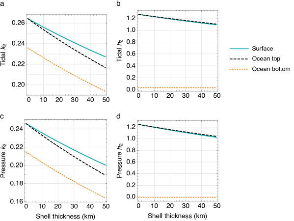
Figure 12: Europa’s tidal and pressure $k_{2}$ and $h_{2}$ Love numbers as a function of shell thickness. We assume a three-layer interior structure with the parameters in Table 1. The core density is calculated self-consistently so as to satisfy the mean density constraint ($\bar{\rho}=3.013$ g cm^-3).

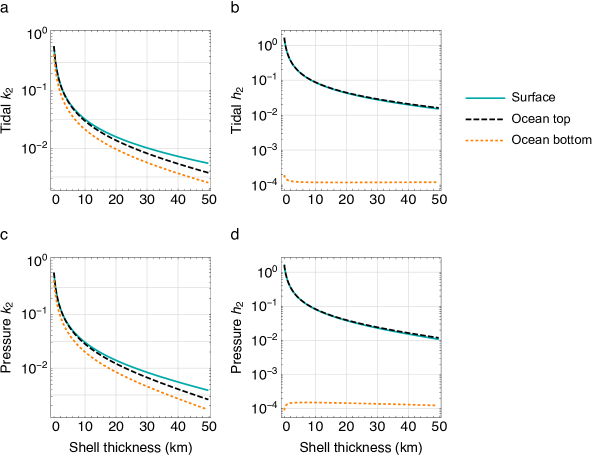
Figure 13: Enceladus’ tidal and pressure $k_{2}$ and $h_{2}$ Love numbers as a function of shell thickness. We assume a three-layer interior structure with the parameters in Table 1. The core density is calculated self-consistently so as to satisfy the mean density constraint ($\bar{\rho}=1.609$ g cm^-3). In panel d, the displacement pressure Love number at the ocean bottom, $h_{2}^{P}(r_{b})$, is negative because a positive pressure potential at the ocean bottom corresponds to a negative radial displacement, and the dotted orange line corresponds to $|h_{2}^{P}(r_{b})|$.

Appendix B Analytic Love number solutions

The propagator matrix method can be used to calculate the Love numbers of bodies with arbitrary interior structures. Although simplified models are less realistic, the analytic solutions for these models provide valuable physical insight.

B.1 Homogeneous interior

Assuming a uniform, incompressible, interior with shear modulus $\mu$ and density $\rho$, the solution vector at the surface is $\mathbf{y}(R)=\mathbf{I}_{c}\mathbf{C}_{c}$, where $\mathbf{I_{c}}$ is given by the first three columns of the matrix in Eq. (1.74) of Sabadini and Vermeersen (2004), and the boundary conditions at the surface yield $\mathbf{C}_{c}=(\mathbf{P}_{1}\mathbf{I}_{c})^{-1}\mathbf{b}$. Thus, the solution vector at the surface can be written as

$$\mathbf{y}(R)=\mathbf{I}_{c}(\mathbf{P}_{1}\mathbf{I}_{c})^{-1}\mathbf{b}.$$ (62)

Using the boundary conditions (28) and the Love number definitions (35),

$$(k_{n}^{T},\,h_{n}^{T},\,\ell_{n}^{T}) =\frac{1}{1+\hat{\mu}}\left\{\frac{3}{2(n-1)},\,\frac{2n+1}{2(n-1)},\,\frac{3}{2n(n-1)}\right\}$$

$$(k_{n}^{L},\,h_{n}^{L},\,\ell_{n}^{L}) =-\frac{1}{1+\hat{\mu}}\left\{1,\,\frac{2n+1}{3},\,\frac{1}{n}\right\}$$

$$(k_{n}^{P},\,h_{n}^{P},\,\ell_{n}^{P}) =(k_{n}^{T},\,h_{n}^{T},\,\ell_{n}^{T})$$ (63)

where

$$\hat{\mu}\equiv\frac{2n^{2}+4n+3}{n}\frac{\mu}{\rho gR}$$ (64)

is a dimensionless effective rigidity. Note that the pressure Love numbers here describe the deformation in response to pressure forcing at the surface of the satellite. The expressions for the tidal and load Love numbers are consistent with those given by Eqs. (2.1.9a)-(2.1.9c) of Lambeck (1980) for $n=2$. We note that Eqs. (5.6.1) and (5.7.1) in Munk and MacDonald (1960) contain typographical errors for the $\ell$ Love numbers.

B.2 Homogeneous thick shell

An incompressible 3-layer body consisting of a core, ocean, and shell is a good toy model for icy satellites with subsurface oceans. If the ocean and shell have the same density, gravitational effects that change with shell thickness can be avoided, providing analytic Love number solutions for arbitrary shell thicknesses. Assuming static tides and a core with infinity rigidity (i.e. non-deformable) (Beuthe, 2018, Eqs. (62) and (L.2)),

$$h_{n}^{T} =\left(\frac{1}{1-\xi_{n}}\right)\left[1+\left(\frac{1}{1-\xi_{n}}\right)z_{h}\frac{\mu}{\rho_{o}gR}\right]^{-1}$$ (65)

where the degree-n density ratio $\xi_{n}$ is given by Eq (11), $g$ is the surface gravity, and $\mu$ is the shear modulus of the shell. The dimensionless factors $z_{h}$ and $z_{\ell}$ depend on $d/R$, where $d$ is the shell thickness (Beuthe, 2018, Eq. (L.5)). For a fluid shell, $\mu=0$ and $h_{n}^{T}=1/(1-\xi_{n})$. At degree 2, $z_{h}$ decreases with shell thickness from $19/5$ for a homogeneous interior to $0$ for the membrane limit of the shell, with an asymptotic behavior $\sim\frac{24}{11}\frac{d}{R}$ (Beuthe, 2015b, Fig. 13). Thus, the concept of the effective rigidity can be generalized from a homogenous body to a body in which a global subsurface ocean decouples the shell from the core if Eq. (64) is modified to

$$\hat{\mu}\equiv\left(\frac{1}{1-\xi_{n}}\right)z_{h}\frac{\mu}{\rho_{o}gR}.$$ (66)

In the homogeneous body limit, $\frac{1}{1-\xi_{n}}=\frac{2n+1}{2(n-1)}$, $z_{h}=\frac{2(n-1)}{2n+1}\frac{2n^{2}+4n+3}{n}$ (Beuthe, 2018, Eq. (L.6)), and Eq. (66) reduces to Eq. (64), as expected. If the shell is thin ($d/R\lesssim 0.2$), the effective rigidity decreases nearly linearly with shell thickness: $z_{h}\sim\frac{6(n-1)(n+2)}{2(n-1)(n+2)+3}\frac{d}{R}$. At degree 2, this approximation underestimates $z_{h}$ by (1, 6, 17)% if the shell thickness is (2, 10, 20)% of the surface radius, respectively. With this definition of the effective rigidity, it is clear that Europa behaves as a ‘soft shell’ body ($\hat{\mu}\lesssim 1$) whereas Enceladus behaves as a ‘hard shell’ body ($\hat{\mu}\gg 1$) (Beuthe, 2018, Section 4.3.2).

Appendix C Numerical solution of the Laplace tidal equations

We extend the method of Matsuyama (2014), based on the method of Longuet-Higgins (1968), to solve the mass and momentum conservation equations (Eqs. (1) and (21)) for ocean tides with an overlying solid shell and no bottom or Navier-Stokes drag ($c_{D}=\nu=0$).

The velocity is specified using a Helmholtz decomposition (Arfken and Weber, 1995, Section 1.16),

$$\mathbf{u}=\nabla\Phi+\nabla\times(\Psi\mathbf{\hat{\mathbf{e}}_{r}})=\hat{\mathbf{e}}_{\theta}\left[r^{-1}\partial_{\theta}\Phi+(r\sin\theta)^{-1}\partial_{\phi}\Psi\right]+\hat{\mathbf{e}}_{\phi}\left[(r\sin\theta)^{-1}\partial_{\phi}\Phi-r^{-1}\partial_{\theta}\Psi\right],$$ (67)

where $\Phi$ has the properties of a potential and $\Psi$ has the properties of a stream function. We expand the forcing potential $U^{T},$ radial tide $\eta$, $\Phi$, and $\Psi$ in spherical harmonics as

$$\eta(r,\,\theta,\,\phi) =\frac{1}{2}\sum_{m=0}^{2}\sum_{n=m}^{\infty}\eta_{nm}(r)Y_{nm}(\theta,\,\phi)e^{-i\omega t}+c.c.$$

$$U^{T}(R,\,\theta,\,\phi) =\frac{1}{2}\sum_{m=0}^{2}\sum_{n=m}^{\infty}U_{nm}^{T}(R)Y_{nm}(\theta,\,\phi)e^{-i\omega t}+c.c.$$

$$\Phi(r,\,\theta,\,\phi) =\frac{1}{2}\sum_{m=0}^{2}\sum_{n=m}^{\infty}\Phi_{nm}(r)Y_{nm}(\theta,\,\phi)e^{-i\omega t}+c.c.$$

$$\Psi(r,\,\theta,\,\phi) =\frac{1}{2}\sum_{m=0}^{2}\sum_{n=m}^{\infty}\Psi_{nm}(r)Y_{nm}(\theta,\,\phi)e^{-i\omega t}+c.c.,$$ (68)

where $\omega=\Omega$ and $\omega=-\Omega$ for the eastward and westward components respectively,

$$Y_{nm}(\theta,\,\phi)\equiv P_{nm}(\cos\theta)e^{im\phi},$$ (69)

$P_{nm}$ are the unnormalized associated Legendre functions define by the Legendre polynomials equation (Arfken and Weber, 1995, Eq. (12.81))

$$P_{nm}(x)=\left(1-x^{2}\right)^{m/2}\frac{d^{m}}{dx^{m}}P_{n}(x),$$ (70)

and $c.c.$ denotes the complex conjugate. Note that this definition of does not include the Condon-Shortley phase factor of $(-1)^{m}$. The nonzero forcing potential coefficients are listed on Table 2.

		Obliquity tide				Eccentricity tide
m		Eastward		Westward		Eastward		Westward
0		-		-		$-(3/2)\Omega^{2}r^{2}e$		-
1		$(1/2)\Omega^{2}r^{2}\theta_{0}$		$(1/2)\Omega^{2}r^{2}\theta_{0}$		-		-
2		-		-		$(7/8)\Omega^{2}r^{2}e$		$-(1/8)\Omega^{2}r^{2}e$

Table 2: Tidal potential expansion coefficients for obliquity ($\theta_{0}$) and eccentricity ($e$) tides (compare Eqs. (5) and (68)). Note that the decomposition into eastward and westward components is irrelevant for $m=0$ and only one coefficient should be used in this case.

Replacing Eqs. (67) and (68) in the LTE and following the procedure outlined in (Longuet-Higgins, 1968) yields

$$\frac{\upsilon_{n}}{2\Omega}U_{nm}^{T} =K_{n}\Im(\Phi_{nm})+b\Re(\Phi_{nm})+p_{\ell+1}\Re(\Psi_{n+1,\,m})+q_{n-1}\Re(\Psi_{n-1,\,m})$$

$$0 =K_{n}\Re(\Phi_{nm})-b\Im(\Phi_{nm})-p_{\ell+1}\Im(\Psi_{n+1,\,m})-q_{n-1}\Im(\Psi_{n-1,\,m})$$

$$0 =L_{n}\Im(\Psi_{nm})+b\Re(\Psi_{nm})-p_{\ell+1}\Re(\Phi_{n+1,\,m})-q_{n-1}\Re(\Phi_{n-1,\,m})$$

$$0 =L_{n}\Re(\Psi_{nm})-b\Im(\Psi_{nm})+p_{\ell+1}\Im(\Phi_{n+1,\,m})+q_{n-1}\Im(\Phi_{n-1,\,m}),$$ (71)

where $\Re$ and $\Im$ denote the real and imaginary parts,

$$b \equiv\frac{\alpha}{2\Omega}$$

$$K_{n} \equiv\lambda+\frac{m}{n(n+1)}-\beta{}_{n}\frac{n(n+1)}{\epsilon\lambda}$$

$$L_{n} \equiv\lambda+\frac{m}{n(n+1)}$$

$$p_{n} \equiv\frac{(n+1)(n+m)}{n(2n+1)}$$

$$q_{n} \equiv\frac{n(n+1-m)}{(n+1)(2n+1)},$$ (72)

$\lambda\equiv\omega/(2\alpha)$, and

$$\epsilon(r)\equiv\frac{4\Omega^{2}r^{2}}{g(R)h_{o}}$$ (73)

is Lamb’s parameter. In Eqs. (71) and (72), $\upsilon_{n}$ and $\beta_{n}$ are given by Eq. (22). The surface ocean solutions can be obtained by replacing $\upsilon_{n}$ and $\beta_{n}$ by $\gamma_{n}^{T}$ and $1-\xi_{2}\gamma_{n}^{L}$ (Eq. (13)), respectively, and evaluating Lamb’s parameter at the surface ($r=R$). Eq. (71) can be written in the more compact form

$$\frac{\upsilon_{n}}{2\Omega}U_{nm}^{T}(R)= -iK_{n}\Phi_{nm}(r)+b\Phi_{nm}(r)+p_{\ell+1}\Psi_{n+1,\,m}(r)+q_{n-1}\Psi_{n-1,\,m}(r)$$

$$0= -iL_{\ell}\Psi_{nm}(r)+b\Psi_{nm}(r)-p_{\ell+1}\Phi_{n+1,\,m}(r)-q_{n-1}\Phi_{n-1,\,m}(r),$$ (74)

which is slightly different from Eq. (A.5) of Matsuyama (2014) due to typographical errors in that paper.

The resonant ocean modes are given by the eigenvalues of the matrices describing Eq. (74). Given the solutions for $\Phi$ and $\Psi$ by solving Eq. (74), the velocity is given by the Helmholtz decomposition (67), where we can use (Arfken and Weber, 1995, p. 725, Eq. (12.87))

$$\partial_{\theta}P_{nm}=\frac{1}{2}(n+m)(n+1-m)P_{n,\,m-1}-\frac{1}{2}P_{n,\,m+1}$$ (75)

to evaluate the $\partial_{\theta}$ derivatives. The radial tide can be found using the mass mass conservation Eq. (1) and the Helmholtz decomposition (67), $i\omega\eta_{nm}=(n(n+1)/r^{2})(h/\omega)\Phi_{nm},$ or

$$\Re(\eta_{nm}(r)) =-\frac{n(n+1)}{r^{2}}\frac{h_{o}}{\omega}\Im(\Phi_{nm}(r))$$

$$\Im(\eta_{nm}(r)) =\frac{n(n+1)}{r^{2}}\frac{h_{o}}{\omega}\Re(\Phi_{nm}(r)).$$ (76)

Given a velocity solution of the Laplace tidal equation, the dissipated energy per unit time and surface area can be found with Eq. (6). Integrating this equation over the tidal forcing period and the satellite surface assuming a thin ocean yields the time- and surface-averaged power,

$$<\dot{E}_{diss}>\equiv r^{2}\int_{0}^{T}dt\int_{0}^{\pi}\int_{0}^{2\pi}d\phi\,d\theta\sin\theta\,F_{diss}=-2\pi\rho_{o}h_{o}\alpha\sum_{m=0}^{2}\sum_{n=m}^{\infty}N_{nm}\left(|\Phi_{nm}(r)|^{2}+|\Psi_{nm}(r)|^{2}\right),$$ (77)

where

$$N_{nm}\equiv\frac{n(n+1)}{2n+1}\frac{(n+m)!}{(n-m)!}$$ (78)

is a normalization constant and the radius can be evaluated at the ocean top ($r=r_{t}$) or bottom ($r=r_{b}$) in the thin ocean limit. Energy conservation requires that the time- and surface-averaged dissipated energy and work done by the tide to be equal (Tyler, 2011; Chen et al., 2014), which allows us to derive the alternative expression

$$<\dot{E}_{diss}>=-2\pi\rho_{o}h_{o}\upsilon_{2}\sum_{m=0}^{2}N_{2m}U_{2m}^{T}(R)\Re(\Phi_{2m}(r)).$$ (79)

Thus, we can verify that our solutions satisfy energy conservation by comparing energy dissipation results using Eqs. (77) and (79), or Eqs. (6) and (79).

Eq (79) is equivalent to Eq. (82) of Beuthe (2016) for thin shells if we take into account the following differences. First, $\upsilon_{2}=\gamma_{2}^{T}+\delta\gamma_{2}^{T}$ in the thin shell limit (Beuthe 2016, Eq. (27); Figure 2). Second, Beuthe (2016) uses normalized spherical harmonics, whereas we use unnormalized spherical harmonics. Third, Beuthe (2016) sums over eastward and westward directions for all $m$, whereas we only include one coefficient for $m=0$ (Table 2). Last, $\Re(\Phi_{2m})=\Im(\tilde{\Phi}_{2m})$ using the notation $\tilde{\Phi}_{nm}=i\Phi_{nm}$ (Beuthe, 2016, Eq. (38)).

Similarly, we can recover Eqs. (26) and (28) of Chen et al. (2014) for a surface ocean using Eqs. (77) and (79) taking into account the following differences. First, Chen et al. (2014) use normalized spherical harmonics, whereas we use unnormalized spherical harmonics. Second, our Fourier expansion coefficients in Eq. (68) are twice as large because Chen et al. (2014) define the Fourier expansion without the factor of $1/2$. Third, Chen et al. (2014) ignore self-gravity and the satellite deformation in response to tidal forcing and surface ocean loading ($\upsilon_{2}=\beta_{n}=1$).

Appendix D Tidal quality factor

We consider an alternative definition of the tidal quality factor,

$$Q\equiv 2\pi\frac{E_{max}}{E_{diss}}$$ (80)

where $E_{max}$ is the maximum kinetic energy of the ocean in the absence of energy dissipation (Hay and Matsuyama, 2017). In this case, it is no longer possible to obtain a simple expression relating the tidal quality factor and the linear drag coefficient. Instead, the tidal quality factor must be calculated after solving the LTE with and without dissipation. Our new definition does not allow for a simple relation between $Q$ and $\alpha$. However, the relevant quantity for computing the effect of tidal heating on the thermal, rotational, and orbital evolution is the energy dissipation rate and our thick shell theory provides a method for computing it.

Using the new definition of $Q$, higher energy dissipation corresponds to smaller $Q$ values (Fig. 14), as expected. $Q$ converges to the prior definition, $Q=\Omega/(2\alpha)$, as the linear drag coefficient decreases because this reduces the effect of dissipation on the kinetic energy. The prior definition results in a tidal quality factor that decreases indefinitely as the linear drag increases. In contrast, our definition introduces natural lower limits. Fig. 14 shows these natural lower limits for obliquity forcing. The natural lower limits for $Q$ also emerge for eccentricity forcing if we consider larger linear drag coefficients.

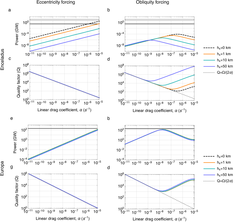
Figure 14: Ocean tidal heating power (energy dissipated in one tidal cycle divided by the tidal forcing period) and tidal quality factor, $Q$, for eccentricity and obliquity forcing as a function of the linear drag coefficient, $\alpha$, for different shell thicknesses, $h_{s}$. Black dashed lines are surface ocean solutions without an overlying solid shell ($h_{s}=0$), and gray dotted lines are the prior definition of the tidal quality factor ($Q=\Omega/(2\alpha)$). The shaded gray region corresponds to the observational constraint of $3.9-18.9$ GW for Enceladus, and the solid horizontal black line is the estimated radiogenic heating power (0.3 GW for Enceladus and 200 GW for Europa). We assume the interior structure parameters in Table 1.

The effect of varying the shell thickness on $Q$ is complex because both the numerator and denominator in Eq. (80) decrease as the shell thickness increases. For the range of linear drag coefficients considered, $Q$ is not sensitive to the shell thickness for eccentricity forcing. For obliquity forcing, the dissipated energy decreases faster than the maximum kinetic energy, resulting in an increase in $Q$ with increasing shell thickness (Figs. 14d and h).

The tidal quality factor for eccentricity forcing reaches small values that imply energy dissipation in one forcing cycle larger than the maximum kinetic energy without dissipation (Figs. 14c and g), which may seem unphysical. However, energy conservation requires the work done on the ocean by the tide-raising potential to be equal to the dissipated energy, and therefore the dissipated energy can be larger than the maximum kinetic energy as long as it is balanced by the work done on the ocean.

Tidal heating increases with the linear drag coefficient, as expected, with the exception of obliquity forcing with high linear drag coefficients (Fig. 14). Eccentricity forcing generates gravity waves, while obliquity forcing generates both gravity and Rossby-Haurwitz waves (Tyler, 2008, 2009, 2011). The tidal heating decrease with increasing linear drag coefficient for the obliquity forcing is associated with Rossby-Haurwitz waves. We verify this by removing the westward traveling component of the obliquity forcing tidal potential (Eq. 5), which prevents the generation of Rossby-Haurwitz waves. In this case, tidal heating increases with the linear drag coefficient.

References

References

- Anderson et al. (1998) Anderson, J.D., Schubert, G., Jacobson, R.A., Lau, E.L., Moore, W.B., Sjogren, W.L., 1998. Europa’s Differentiated Internal Structure: Inferences from Four Galileo Encounters. Science 281, 2019–2022. doi:10.1126/science.281.5385.2019.
- Arfken and Weber (1995) Arfken, G., Weber, H., 1995. Mathematical methods for physicists. Fourth ed., Academic Press.
- Baland et al. (2016) Baland, R.M., Yseboodt, M., Van Hoolst, T., 2016. The obliquity of Enceladus. Icarus 268, 12–31. doi:10.1016/j.icarus.2015.11.039.
- Běhounková et al. (2012) Běhounková, M., Tobie, G., Choblet, G., Čadek, O., 2012. Tidally-induced melting events as the origin of south-pole activity on Enceladus. Icarus 219, 655–664. doi:10.1016/j.icarus.2012.03.024.
- Beuthe (2013) Beuthe, M., 2013. Spatial patterns of tidal heating. Icarus 223, 308–329. doi:10.1016/j.icarus.2012.11.020.
- Beuthe (2015a) Beuthe, M., 2015a. Tidal Love numbers of membrane worlds: Europa, Titan, and Co. Icarus 258, 239–266. doi:10.1016/j.icarus.2015.06.008.
- Beuthe (2015b) Beuthe, M., 2015b. Tides on Europa: The membrane paradigm. Icarus 248, 109–134. doi:10.1016/j.icarus.2014.10.027.
- Beuthe (2016) Beuthe, M., 2016. Crustal control of dissipative ocean tides in Enceladus and other icy moons. Icarus 280, 278–299. doi:10.1016/j.icarus.2016.08.009.
- Beuthe (2018) Beuthe, M., 2018. Enceladus’s crust as a non-uniform thin shell: I tidal deformations. Icarus 302, 145–174. doi:10.1016/j.icarus.2017.11.009.
- Beuthe et al. (2016) Beuthe, M., Rivoldini, A., Trinh, A., 2016. Enceladus’s and Dione’s floating ice shells supported by minimum stress isostasy. Geophys. Res. Lett. 43, 10088–10096. doi:10.1002/2016GL070650.
- Bills (2005) Bills, B.G., 2005. Free and forced obliquities of the Galilean satellites of Jupiter. Icarus 175, 233–247. doi:10.1016/j.icarus.2004.10.028.
- Chen and Nimmo (2011) Chen, E.M.A., Nimmo, F., 2011. Obliquity tides do not significantly heat Enceladus. Icarus 214, 779–781. doi:10.1016/j.icarus.2011.06.007.
- Chen and Nimmo (2016) Chen, E.M.A., Nimmo, F., 2016. Tidal dissipation in the lunar magma ocean and its effect on the early evolution of the Earth-Moon system. Icarus 275, 132–142. doi:10.1016/j.icarus.2016.04.012.
- Chen et al. (2014) Chen, E.M.A., Nimmo, F., Glatzmaier, G.A., 2014. Tidal heating in icy satellite oceans. Icarus 229, 11–30. doi:10.1016/j.icarus.2013.10.024.
- Dahlen and Tromp (1998) Dahlen, F., Tromp, J., 1998. Theoretical Global Seismology. Princeton University Press.
- Egbert and Ray (2000) Egbert, G.D., Ray, R.D., 2000. Significant dissipation of tidal energy in the deep ocean inferred from satellite altimeter data. Nature 405, 775–778. doi:10.1038/35015531.
- Egbert and Ray (2001) Egbert, G.D., Ray, R.D., 2001. Estimates of M2 tidal energy dissipation from TOPEX/Poseidon altimeter data. Journal of Geophysical Research: Oceans 106, 22475–22502. doi:10.1029/2000JC000699.
- Fischer and Spohn (1990) Fischer, H.J., Spohn, T., 1990. Thermal-orbital histories of viscoelastic models of Io (J1). Icarus 83, 39–65. doi:10.1016/0019-1035(90)90005-T.
- Gao and Stevenson (2013) Gao, P., Stevenson, D.J., 2013. Nonhydrostatic effects and the determination of icy satellites’ moment of inertia. Icarus 226, 1185–1191. doi:10.1016/j.icarus.2013.07.034.
- Goldreich and Soter (1966) Goldreich, P., Soter, S., 1966. Q in the Solar System. Icarus 5, 375–389.
- Green and Nycander (2013) Green, J.A.M., Nycander, J., 2013. A Comparison of Tidal Conversion Parameterizations for Tidal Models. Journal of Physical Oceanography 43, 104–119. doi:10.1175/JPO-D-12-023.1.
- Hammond et al. (2018) Hammond, N.P., Barr, A.C., Cooper, R.F., Caswell, T.E., Hirth, G., 2018. Experimental Constraints on the Fatigue of Icy Satellite Lithospheres by Tidal Forces. J. Geophys. Res. 123, 390–404. doi:10.1002/2017JE005464.
- Hartkorn and Saur (2017) Hartkorn, O., Saur, J., 2017. Induction signals from Callisto’s ionosphere and their implications on a possible subsurface ocean. Journal of Geophysical Research: Space Physics 122, 11677–11697. doi:10.1002/2017JA024269.
- Hay and Matsuyama (2017) Hay, H.C.F.C., Matsuyama, I., 2017. Numerically modelling tidal dissipation with bottom drag in the oceans of Titan and Enceladus. Icarus 281, 342–356. doi:10.1016/j.icarus.2016.09.022.
- Hedman et al. (2013) Hedman, M.M., Gosmeyer, C.M., Nicholson, P.D., Sotin, C., Brown, R.H., Clark, R.N., Baines, K.H., Buratti, B.J., Showalter, M.R., 2013. An observed correlation between plume activity and tidal stresses on Enceladus. Nature 500, 182–184. doi:10.1038/nature12371.
- Hendershott (1972) Hendershott, M.C., 1972. The Effects of Solid Earth Deformation on Global Ocean Tides. Geophysical Journal 29, 389–402. doi:10.1111/j.1365-246X.1972.tb06167.x.
- Hinderer (1986) Hinderer, J., 1986. Resonance Effects of the Earth’s Fluid Core, in: Earth Rotation: Solved and Unsolved Problems. Springer, Dordrecht, Dordrecht, pp. 277–296. doi:10.1007/978-94-009-4750-4_20.
- Hinderer and Legros (1989) Hinderer, J., Legros, H., 1989. Elasto-Gravitational Deformation, Relative Gravity Changes and Earth dynamics. Geophysical Journal International 97, 481–495. doi:10.1111/j.1365-246X.1989.tb00518.x.
- Howett et al. (2011) Howett, C.J.A., Spencer, J.R., Pearl, J., Segura, M., 2011. High heat flow from Enceladus’ south polar region measured using 10-600 cm-1 Cassini/CIRS data. J. Geophys. Res. 116, E03003. doi:10.1029/2010JE003718.
- Hussmann and Spohn (2004) Hussmann, H., Spohn, T., 2004. Thermal-orbital evolution of Io and Europa. Icarus 171, 391–410. doi:10.1016/j.icarus.2004.05.020.
- Iess et al. (2012) Iess, L., Jacobson, R.A., Ducci, M., Stevenson, D.J., Lunine, J.I., Armstrong, J.W., Asmar, S.W., Racioppa, P., Rappaport, N.J., Tortora, P., 2012. The Tides of Titan. Science 337, 457–459. doi:10.1126/science.1219631.
- Jara-Orué and Vermeersen (2011) Jara-Orué, H.M., Vermeersen, B.L.A., 2011. Effects of low-viscous layers and a non-zero obliquity on surface stresses induced by diurnal tides and non-synchronous rotation: The case of Europa. Icarus 215, 417–438. doi:10.1016/j.icarus.2011.05.034.
- Jayne and St Laurent (2001) Jayne, S.R., St Laurent, L.C., 2001. Parameterizing tidal dissipation over rough topography. Geophys. Res. Lett. 28, 811–814. doi:10.1029/2000GL012044.
- Kamata et al. (2016) Kamata, S., Kimura, J., Matsumoto, K., Nimmo, F., Kuramoto, K., Namiki, N., 2016. Tidal deformation of Ganymede: Sensitivity of Love numbers on the interior structure. J. Geophys. Res. 121, 1362–1375. doi:10.1002/2016JE005071.
- Kamata et al. (2015) Kamata, S., Matsuyama, I., Nimmo, F., 2015. Tidal resonance in icy satellites with subsurface oceans. J. Geophys. Res. Planets 120, 1528–1542. doi:10.1002/2015JE004821.
- Kivelson et al. (2000) Kivelson, M.G., Khurana, K.K., Russell, C.T., Volwerk, M., Walker, R.J., Zimmer, C., 2000. Galileo Magnetometer Measurements: A Stronger Case for a Subsurface Ocean at Europa. Science 289, 1340–1343. doi:10.1126/science.289.5483.1340.
- Kivelson et al. (2002) Kivelson, M.G., Khurana, K.K., Volwerk, M., 2002. The Permanent and Inductive Magnetic Moments of Ganymede. Icarus 157, 507–522. doi:10.1006/icar.2002.6834.
- Lamb (1993) Lamb, H., 1993. Hydrodynamics. 6 ed., Cambridge University Press, Cambridge.
- Lambeck (1980) Lambeck, K., 1980. The earth’s variable rotation: Geophysical causes and consequences. Cambridge University Press, Cambridge.
- Longuet-Higgins (1968) Longuet-Higgins, M.S., 1968. The Eigenfunctions of Laplace’s Tidal Equations over a Sphere. Philosophical Transactions of the Royal Society A: Mathematical, Physical and Engineering Sciences 262, 511–607. doi:10.1098/rsta.1968.0003.
- Matsuyama (2014) Matsuyama, I., 2014. Tidal dissipation in the oceans of icy satellites. Icarus 242, 11–18. doi:10.1016/j.icarus.2014.07.005.
- McKinnon (2015) McKinnon, W.B., 2015. Effect of Enceladus’s rapid synchronous spin on interpretation of Cassini gravity. Geophys. Res. Lett. 42, 2137–2143. doi:10.1002/2015GL063384.
- Moore and Schubert (2000) Moore, W.B., Schubert, G., 2000. NOTE: The Tidal Response of Europa. Icarus 147, 317–319. doi:10.1006/icar.2000.6460.
- Munk and MacDonald (1960) Munk, W.H., MacDonald, G.J.F., 1960. The rotation of the earth; a geophysical discussion. Cambridge University Press, Cambridge.
- Nimmo and Bills (2010) Nimmo, F., Bills, B.G., 2010. Shell thickness variations and the long-wavelength topography of Titan. Icarus 208, 896–904. doi:10.1016/j.icarus.2010.02.020.
- Nimmo and Pappalardo (2016) Nimmo, F., Pappalardo, R.T., 2016. Ocean worlds in the outer solar system. J. Geophys. Res. 121, 1378–1399. doi:10.1002/2016JE005081.
- Nimmo et al. (2014) Nimmo, F., Porco, C., Mitchell, C., 2014. Tidally Modulated Eruptions on Enceladus: Cassini ISS Observations and Models. Astronomical Journal 148, 46. doi:10.1088/0004-6256/148/3/46.
- Nimmo et al. (2007) Nimmo, F., Thomas, P.C., Pappalardo, R.T., Moore, W.B., 2007. The global shape of Europa: Constraints on lateral shell thickness variations. Icarus 191, 183–192. doi:10.1016/j.icarus.2007.04.021.
- Ojakangas (1989a) Ojakangas, G., 1989a. Polar wander of an ice shell on Europa. Icarus 81, 242–270. doi:10.1016/0019-1035(89)90053-5.
- Ojakangas (1989b) Ojakangas, G., 1989b. Thermal state of an ice shell on Europa. Icarus 81, 220–241. doi:10.1016/0019-1035(89)90052-3.
- Ojakangas and Stevenson (1986) Ojakangas, G.W., Stevenson, D.J., 1986. Episodic volcanism of tidally heated satellites with application to Io. Icarus 66, 341–358. doi:10.1016/0019-1035(86)90163-6.
- Peltier (1974) Peltier, W.R., 1974. The Impulse Response of a Maxwell Earth. Rev. Geophys. Space Phys. 12, 649–669. doi:10.1029/RG012i004p00649.
- Ross and Schubert (1990) Ross, M.N., Schubert, G., 1990. The coupled orbital and thermal evolution of Triton. Geophys. Res. Lett. 17, 1749–1752. doi:10.1029/GL017i010p01749.
- Sabadini and Vermeersen (2004) Sabadini, R., Vermeersen, B., 2004. Global Dynamics of the Earth: Applications of Normal Mode Relaxation Theory to Solid-Earth Geophysics. Kluwer Academic Publishers.
- Sagan and Dermott (1982) Sagan, C., Dermott, S.F., 1982. The tide in the seas of Titan. Nature 300, 731–733. doi:10.1038/300731a0.
- Saito (1974) Saito, M., 1974. Some problems of static deformation of the earth. Journal of Physics of the Earth 22, 123–140. doi:10.4294/jpe1952.22.123.
- Sasao et al. (1980) Sasao, T., Okubo, S., Saito, M., 1980. A simple theory on the dynamical effects of a stratified fluid core upon nutational motion of the Earth, in: Proceedings of the International Astronomical Union, pp. 165–183. doi:10.1017/S0074180900032009.
- Sasao and Wahr (1981) Sasao, T., Wahr, J.M., 1981. An excitation mechanism for the free ’core nutation’. Geophysical Journal 64, 729–746. doi:10.1111/j.1365-246X.1981.tb02692.x.
- Saur et al. (2015) Saur, J., Duling, S., Roth, L., Jia, X., Strobel, D.F., Feldman, P.D., Christensen, U.R., Retherford, K.D., McGrath, M.A., Musacchio, F., Wennmacher, A., Neubauer, F.M., Simon, S., Hartkorn, O., 2015. The search for a subsurface ocean in Ganymede with Hubble Space Telescope observations of its auroral ovals. Journal of Geophysical Research: Space Physics 120, 1715–1737. doi:10.1002/2014JA020778.
- Showman et al. (1997) Showman, A.P., Stevenson, D.J., Malhotra, R., 1997. Coupled Orbital and Thermal Evolution of Ganymede. Icarus 129, 367–383. doi:10.1006/icar.1997.5778.
- Sohl et al. (1995) Sohl, F., Sears, W.D., Lorenz, R.D., 1995. Tidal dissipation on Titan. Icarus 115, 278–294. doi:10.1006/icar.1995.1097.
- Spencer et al. (2013) Spencer, J.R., Howett, C.J.A., Verbiscer, A., Hurford, T.A., Segura, M., Spencer, D.C., 2013. Enceladus Heat Flow from High Spatial Resolution Thermal Emission Observations, in: European Planetary Science Congress 2013, pp. EPSC2013–840–1.
- Spencer et al. (2006) Spencer, J.R., Pearl, J.C., Segura, M., Flasar, F.M., Mamoutkine, A., Romani, P., Buratti, B.J., Hendrix, A.R., Spilker, L.J., Lopes, R.M.C., 2006. Cassini Encounters Enceladus: Background and the Discovery of a South Polar Hot Spot. Science 311, 1401–1405. doi:10.1126/science.1121661.
- Spohn and Schubert (2003) Spohn, T., Schubert, G., 2003. Oceans in the icy Galilean satellites of Jupiter? Icarus 161, 456–467. doi:10.1016/S0019-1035(02)00048-9.
- Takeuchi and Saito (1972) Takeuchi, H., Saito, M., 1972. Seismic surface waves, in: Bolt, B.A. (Ed.), Methods in Computational Physics. Academic Press, New York,, pp. 217–295. doi:10.1016/B978-0-12-460811-5.50010-6.
- Thomas et al. (2016) Thomas, P.C., Tajeddine, R., Tiscareno, M.S., Burns, J.A., Joseph, J., Loredo, T.J., Helfenstein, P., Porco, C., 2016. Enceladus’s measured physical libration requires a global subsurface ocean. Icarus 264, 37–47. doi:10.1016/j.icarus.2015.08.037.
- Tobie et al. (2005) Tobie, G., Grasset, O., Lunine, J.I., Mocquet, A., Sotin, C., 2005. Titan’s internal structure inferred from a coupled thermal-orbital model. Icarus 175, 496–502. doi:10.1016/j.icarus.2004.12.007.
- Tyler (2014) Tyler, R., 2014. Comparative estimates of the heat generated by ocean tides on icy satellites in the outer Solar System. Icarus 243, 358–385. doi:10.1016/j.icarus.2014.08.037.
- Tyler (2008) Tyler, R.H., 2008. Strong ocean tidal flow and heating on moons of the outer planets. Nature 456, 770–772. doi:10.1038/nature07571.
- Tyler (2009) Tyler, R.H., 2009. Ocean tides heat Enceladus. Geophys. Res. Lett. 36, L15205.
- Tyler (2011) Tyler, R.H., 2011. Tidal dynamical considerations constrain the state of an ocean on Enceladus. Icarus 211, 770–779. doi:10.1016/j.icarus.2010.10.007.
- Wahr et al. (2009) Wahr, J., Selvans, Z.A., Mullen, M.E., Barr, A.C., Collins, G.C., Selvans, M.M., Pappalardo, R.T., 2009. Modeling stresses on satellites due to nonsynchronous rotation and orbital eccentricity using gravitational potential theory. Icarus 200, 188–206. doi:10.1016/j.icarus.2008.11.002.
- Wahr et al. (2006) Wahr, J.M., Zuber, M.T., Smith, D.E., Lunine, J.I., 2006. Tides on Europa, and the thickness of Europa’s icy shell. J. Geophys. Res. 111, E12005. doi:10.1029/2006JE002729.
- Webb (1980) Webb, D.J., 1980. Tides and tidal friction in a hemispherical ocean centred at the equator. Geophysical Journal International 61, 573–600. doi:10.1111/j.1365-246X.1980.tb04833.x.
- Zimmer et al. (2000) Zimmer, C., Khurana, K.K., Kivelson, M.G., 2000. Subsurface Oceans on Europa and Callisto: Constraints from Galileo Magnetometer Observations. Icarus 147, 329–347. doi:10.1006/icar.2000.6456.
- Zschau (1978) Zschau, J., 1978. Tidal Friction in the Solid Earth: Loading Tides Versus Body Tides, in: Tidal Friction and the Earth’s Rotation. Springer, Berlin, Heidelberg, Berlin, Heidelberg, pp. 62–94. doi:10.1007/978-3-662-40203-0_7.