Simultaneous long-term monitoring of LS I by OVRO and Fermi-LAT
Abstract
Previous long-term monitorings of the -ray-loud X-ray binary LS I have revealed the presence of a long-term modulation of years. After nine years of simultaneous monitoring of LS I by the Owens Valley Radio Observatory and the Fermi-LAT, two cycles of the long-term period are now available. Here we perform timing-analysis on the radio and the -ray light curves. We confirm the presence of previously detected periodicities at both radio and GeV -ray wavelengths. Moreover, we discover an offset of the long-term modulation between radio and -ray data which could imply different locations of the radio (15 GHz) and GeV emission along the precessing jet.
keywords:
Radio continuum: stars - X-rays: binaries - X-rays: individual (LS I ) - Gamma-rays: stars1 Introduction
The stellar system LS I is detected all over the electromagnetic spectrum ranging from radio to very high energy -rays (Taylor & Gregory, 1982; Paredes et al., 1994; Mendelson & Mazeh, 1989; Zamanov et al., 1999; Harrison et al., 2000; Abdo et al., 2009; Albert et al., 2006). The binary consists of a Be type star (Casares et al., 2005) and a compact object in an eccentric orbit. Optical polarization observations have determined a value of 25 degrees for the position angle of the rotational axis of the Be disk in LS I (Nagae et al., 2006). Assuming that the inclination angle of the orbit coincides with the position angle of the rotational axis of the Be star, for an inclination angle of 25 degrees the compact object would be a black hole (e.g., Casares et al., 2005). Indeed the X-ray characteristics of LS I fit well those of accreting black holes (Massi et al., 2017), and not those of a radio pulsar, which is the alternative suggested model for LS I (e.g., Dubus, 2006).
By Bayesian analysis of 20 years of radio data Gregory (2002) determined the orbital period, d. Lomb-Scargle timing analysis (Lomb, 1976; Scargle, 1982) of 37 years of radio data resulted in the detection of a second period d (Massi & Torricelli-Ciamponi, 2016) consistent with a previously determined precession period of the radio jet mapped in VLBI images (Massi et al., 2012). Recently VLBA astrometry increased the accuracy to d (Wu et al., 2017).
The presence of a very stable long-term flux modulation affecting the radio emission (Massi & Torricelli-Ciamponi, 2016) finds a straightforward explanation as being the result of the beating between the two intrinsic and stable orbital and precession periodicities and (Massi & Jaron, 2013). For d and the last determination by Wu et al. (2017) of d the beating (i.e., ) results in d. This hypothesis was tested by Massi & Torricelli-Ciamponi (2014) who developed a physical model (based on the work of Kaiser 2006) of a self-absorbed jet, periodically () refilled with electrons, and which precesses with a period of and thus continuously changes angle with respect to the line of sight of an observer, giving rise to periodic changes in the Doppler boosting of the intrinsic emission. The model by Massi & Torricelli-Ciamponi (2014) reproduces the observed radio light curve over the last four decades. The alternative scenario in which the long-term modulation could be the result of changes in the Be star wind is unlikely. The unstable quasi-periodic behavior of Be stars has been reviewed by Rivinius et al. (2013), and we refer to the introduction of Jaron et al. (2017) for a discussion of this issue in comparison to the very stable periodic behavior of LS I .
In the GeV regime (as continously monitored by the Large Area Telescope onboard the Fermi satellite, i.e., Fermi-LAT, Atwood et al. 2009), the orbital period was clearly detected first by Abdo et al. (2009). However, as found out by Ackermann et al. (2013), the behavior around periastron differs from that around apastron in the way that the long-term modulation only affects the latter and not the former. In agreement with these findings, Jaron & Massi (2014) report the GeV emission around apastron to be further modulated by the precession period , known from the radio emission. By extending the physical model of Massi & Torricelli-Ciamponi (2014) to the GeV regime, including both synchrotron self-Compton and external inverse Compton, Jaron et al. (2016) reproduce the radio and GeV light curves and their different timing characteristics at periastron and apastron.
While the stability of the two periodicities and could be well demonstrated for the radio regime on the basis of almost 40 years of data, corresponding to more than eight cycles of the long-term modulation, continuous monitoring of LS I in the GeV regime has only been ongoing since 2008. The now completed two long-term cycles of Fermi-LAT observations and the availability of almost simultaneous radio monitoring by the Owens Valley Radio Observatory (OVRO) allows us to investigate on different influences of the two periodicities and , and their beating, in the radio and GeV emission.
2 Observations

2.1 OVRO
The OVRO has been monitoring LS I at 15 GHz since 2009 March 18 (MJD 54908) with an average cadence of 5.8 days, i.e., well above the Nyquist limit of the periodicities of months to years considered here. The telescope uses off-axis dual-beam optics and a cryogenic receiver with 3 GHz bandwidth centred at 15 GHz. Atmospheric and ground contributions as well as gain fluctuations are removed with the double switching technique (Readhead et al., 1989) where the observations are conducted in an ON-ON fashion so that one of the beams is always pointed on the source. Until May 2014 the two beams were rapidly alternated using a Dicke switch, since May 2014 when a new pseudo-correlation receiver replaced the old receiver a 180 degree phase switch is used. Relative calibration is obtained with a temperature-stable noise diode to compensate for gain drifts. The primary flux density calibrator is 3C 286 with an assumed value of 3.44 Jy (Baars et al., 1977), DR21 is used as secondary calibrator source. Details of the observation and data reduction schemes are given in Richards et al. (2011).
In order to increase the signal to noise ratio, we only include data above in the analysis. In the bottom panel of Fig. 1 the light curve resulting from these observations is plotted. Covering a long-term phase interval of (for d, see second -axis in the upper panel) two cycles of the long-term modulation have now been monitored by OVRO. The long-term modulation is clearly visible in this plot. During the maximum of the long-term modulation there is a time interval (MJD 56400–56550) of 140 d (i.e., six orbital cycles of d) very poorly sampled: There are only seven observations, which in addition do not coincide with radio outbursts as predicted by Jaron & Massi (2013).
2.2 Fermi-LAT
The Fermi-LAT data used for the analysis presented here cover the time from MJD 54682–58015 (i.e., August 4 2008 until September 19 2017). In order to compute a light curve from the Pass 8 photon data downloaded from the Fermi-LAT data server111https://fermi.gsfc.nasa.gov/cgi-bin/ssc/LAT/LATDataQuery.cgi we include all data within 10∘ around the position of LS I and use version v10r0p5 of the Fermi ScienceTools222Available from https://fermi.gsfc.nasa.gov/ssc/data/analysis/software/ to fit the source with a log-parabola,
| (1) |
with all parameters left free for the fit. All parameters of all other sources within 10∘ are left free as well. Sources between 10 and 15∘ are included in the analysis with their parameters fixed to the catalog values. The diffuse emission was modeled using the Galactic model file gll_iem_v06.fits, and the isotropic spectral template iso_P8R2_SOURCE_V6_v06.txt. We perform this fit, restricted to the energy range GeV, for every time bin of width one day.
3 Results
3.1 Timing analysis
We perform Lomb-Scargle timing analysis (Lomb, 1976; Scargle, 1982) on the OVRO and Fermi-LAT data, using the UK Starlink software package in the same way as described in Massi & Jaron (2013).
The orbital phase of LS I is defined as
| (2) |
where MJD (Gregory, 2002). Periastron occurs in this case at (Casares et al., 2005), i.e., not at zero orbital phase as is usual for binary systems. The long-term phase is defined as
| (3) |
| Fermi-LAT |
|---|
| Periastron |
| = |
| Apastron |
| = |
| = |
| = |
| OVRO |
| = |
| = |
| = |
3.1.1 OVRO

The results of the timing analysis of the OVRO data are shown in Fig. 2. In the entire observed light curve (panel a) there is a clear signal at the orbital period and the long-term period. The zoom on the orbital period in panel b shows two peaks, i.e., the orbital period and the precession period . The values of the detected periods are listed in the lower part of Table 1.
3.1.2 Fermi-LAT

Since the GeV emission from LS I has different timing characteristics at periastron and apastron (Ackermann et al., 2013; Jaron & Massi, 2014; Jaron et al., 2016), we divided the light curve into (periastron), and (apastron).
The Lomb-Scargle periodograms for the Fermi-LAT data are presented in Fig. 3. Panel a and the zoom in b show a peak at the orbital period . Panel c, showing the result for the apastron data, contains a well pronounced peak at the position of the long-term period, and the zoom in panel d shows two significant peaks, at the orbital period and precession period . The values of the detected periods can be found in the upper part of Table 1.
3.2 Folding the data
All of the periods found by the timing analysis, presented in Table 1, are in agreement with the values reported before in the literature (see Sect. 1). For the folding of the radio and -ray light curves we use the following values: d (Gregory, 2002) for the orbit, d (Wu et al., 2017) for the precession, and
| (4) |
resulting as the beat period of the orbital and precession periods.
3.2.1 OVRO
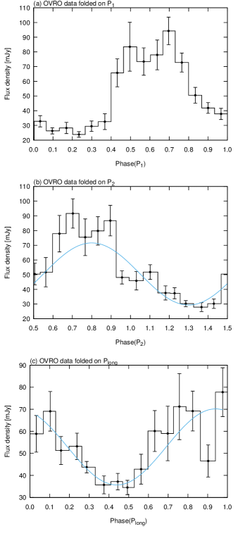
Folding the OVRO data on results in the plot shown in Fig. 4 a, the radio emission peaking from orbital phases , i.e., around apastron, while at periastron the radio flux reaches only mJy. This is in agreement with earlier observations at different radio frequencies (Massi & Torricelli-Ciamponi, 2016, and references therein). The radio data folded with and are shown in Figs 4 b and c, respectively. The peak for the radio data folded with is at whereas radio data folded with have a minimum at 0.45, i.e., maximum at 0.95.
3.2.2 Fermi-LAT
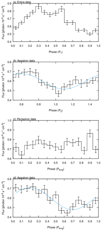
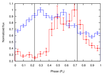
In Fig. 5 a the GeV data are folded on the orbital period , showing that the emission covers the whole orbit. Figure 6 shows the overlay with the radio emission, both normalized to their maximum fluxes for a better comparability of the two. In this plot it is evident that the radio emission is confined to orbital periods around apastron while the GeV emission covers the entire orbit.
Figures 5 b and d present the apastron data folded on the precession period and the long-term period , respectively. As already pointed out by Ackermann et al. (2013) the GeV emission is only affected by the long-term modulation around apastron, and indeed only the plot in panel d shows a significant modulation for , while the plot in Fig. 5 c does not show any significant modulation. The peak of in the folded apastron data is at whereas the peak for apastron data folded with is at .
3.2.3 Phase-offsets between radio and GeV
| d | ||||
| Fermi-LAT | 1.09 | |||
| OVRO | 2.40 | |||
| d | ||||
| Fermi-LAT | 2.12 | |||
| OVRO | 1.17 |
When folding the data on the periods and , as presented in Figs 4 b and c for the OVRO data, and in Figs 5 b and d for the Fermi-LAT apastron data, there is an offset between the otherwise similar shapes of the two. Aimed at investigating this phase-offset we fit the folded data with a sine function of the form
| (5) |
The parameters resulting from this fit are presented in Table 2 and the corresponding curves are plotted as blue solid lines in Figs 4 b and c, and Figs 5 b and d. The phase-offset is then given by
| (6) | |||||
| (7) |
for and , respectively.
As outlined in Appendix A, a phase-offset of the lower of the two frequencies ( in our case) giving rise to a beating results in the long-term modulation to be offset in phase by the negative value . This explains the different sign in the offsets and the fact that the sum of the two observed phase-offsets
| (8) |
is not significantly different from zero.
4 Comparison with previous results
In this section we compare our results of two long-term cycles of Fermi-LAT data with results that Xing et al. (2017, X17 hereafter) obtained by analysing a Fermi-LAT data set covering a very similar time span. In particular we discuss their results of a peak shift and of a dip.
In our Fig. 5 we plot periastron and apastron data for the energy range 0.1 - 3 GeV. X17 show in the top panel of their Fig. 5 a plot of a subset for periastron, , and a subset for apastron, for data 5.5 GeV and for a slightly different long-term period, i.e. 1667 d, instead of our 1659 d (compatible within their uncertainty). Despite the slightly different periods used for the folding, energy interval and orbital phase intervals, our plots and the plot by X17 are consistent. They show the absence of long-term modulation at periastron and the presence of a long-term modulation at apastron, peaking in Fig. 5 top right panel in X17 at superorbital phase about and in the bottom panel of our Fig. 5 around .
Besides, X17 show in the right column of their Fig. 3 data of the energy range 0.1-300 GeV folded on their long-term period of 1667 d for small subsets of data: a single bin of orbital phase . The apastron data (right column of their Fig. 3) indeed show a significant folding and in each fit the peak results constant at the same superorbital phase (from their Table 3). This value is well consistent with the peak at of their Fig. 5, top right panel, as discussed above, and with our value of . The constant value of the peak phase for apastron data is shown in the bottom panel of Fig. 4 in X17. This means that for apastron data there is no shift of the peak phase.
Different is the result for periastron data. At periastron there is no long-term spectral feature in our spectrum shown in Fig. 3 a, neither a folding in both our Fig. 5 c nor in the top left panel of Fig. 5 in X17. They fit the data (their Fig. 3, left column) nevertheless with a sine function and discuss the found large . The fact that the resulting peak phase appears at different phases going from to , i.e., their called “shift” (their Table 3 and the bottom panel of their Fig. 4) just reflects indeed the noise-dominated fit.
Finally, X17 show in their Fig. 3, left column, that in the periastron data folded on a period of 1667 d there appears a “dip” at superorbital phase , the same in their Fig. 5, top right. However, the dip occurs at only one bin. Its noisy nature is clear when it disappears in data folded with a slightly different period: our Fig. 5 c, folded with 1659 d does not show any dip at about .
5 Discussion
The observed flux density from a relativistic jet (Mirabel & Rodríguez, 1999) is the product of an intrinsically variable jet that depends on the orbital period and Doppler boosting (DB) towards the observer that depends on the jet precession period . In the physical model for LS I (Massi & Torricelli-Ciamponi, 2014; Jaron et al., 2016) this implies
| (9) |
The DB factor depends on the jet velocity and as discussed in Jaron et al. (2016) the low velocity of the jet at periastron, Comptoinized before the acceleration region, explains the dependence of GeV emission at periastron on only and the lack of any radio outburst (i.e., electrons ejected in the strong stellar UV radiation suffer catastrophic inverse Compton losses). At apastron the larger distance from the stellar radiation field, and consequently lower inverse Compton losses for the electrons, results in the radio and GeV emission to be both affected by the term. Our result of an offset for between radio and GeV emission implies a different angle with respect to the line of sight for the radio (15 GHz) jet and GeV jet. In fact a different angle induces a different DB and therefore a different phase in the long term modulation. The maximum amplitude corresponds to an alignement of and , i.e., the emitting electrons are ejected at the minimum angle with respect to the line of sight.
A model analogous to the scenario in which Lisakov et al. (2017) explain observed time lags between radio and -ray emission in active galactic nucleus 3C 273, could qualitatively explain the here observed phase-shift between the radio and -ray emission, as sketched in Fig. 7. Particles are ejected into the jet in one direction, and at time these high-energy particles emit -ray emission via the inverse Compton process (left part of the sketch). Here the bulk flow is aligned with the line-of-sight (LoS) and the -ray emission is maximally Doppler boosted333In general the maximum Doppler boosting occurs when the bulk motion encloses the smallest angle with the line-of-sight and is not necessarily perfectly aligned.. Later (right part of the sketch), those particles have moved further down the jet with the bulk velocity. The emission region has expanded and cooled and now those particles emit 15 GHz synchrotron emission. This bulk flow is still aligned with the LoS and now the 15 GHz emission is maximally boosted. At the same time new particles that have been ejected into a different direction due to jet precession emit -rays at time . But now the bulk flow of this new population is less aligned with the LoS and the emission is less boosted. Imagining this as a continuous process (and not discrete as in the simplified sketch), naturally leads to the phase-offset in the Doppler boosting () for radio and -rays, and consequently also for . The implications are:
-
1.
A displacement of the -ray and radio emission regions along the jet naturally explains the phase-offset as a phase-offset in the Doppler boosting.
-
2.
The phase-shift relates to a distance between the -ray emission region and the 15 GHz emission region along the jet.
6 Conclusions
The X-ray binary LS I features highly periodic emission all over the electromagntic spectrum, one period being a long-term modulation of d (e.g., Massi & Torricelli-Ciamponi, 2016). The Fermi-LAT monitoring the entire sky in the GeV since 2008 (Atwood et al., 2009), has now completed two of these long-term cycles of LS I . We performed timing analysis on the Fermi-LAT light curve and the simultanous radio data at 15 GHz obtained by long-term OVRO monitoring. We were aimed to compare the characteristics of the radio and GeV emission. These are our conclusions.
-
1.
GeV emission covers the whole orbit whereas radio emission is confined only around apastron (Fig. 6), confirming the result of Jaron et al. (2016).
-
2.
Whereas GeV emission around periastron is only modulated with , both orbital period and precession period are present in both radio and apastron GeV data. This also confirms the result of Jaron et al. (2016).
-
3.
The here presented analysis yields the new result that when folding data with there is a phase-offset between radio and GeV data of .
-
4.
The long-term modulation () of the flux is present in both radio and apastron GeV data. When data are folded with this period there is an offset between radio GeV data of .
-
5.
The different sign of the offsets of and is as predicted from the beating (see Appendix A).
-
6.
A model as outlined in Sect. 5 is able to qualitatively explain the here observed phase-shift between the radio and GeV emission from LS I , implying that the GeV emission region is upstream from the site of radio emission. Further long-term monitoring of LS I at multiple wavelengths and physical modelling are necessary to quantitatively test this hypothesis.
Acknowledgements
We thank Eduardo Ros for reading the manuscript. FJ thanks Walter Alef and Helge Rottmann for granting computing time at the MPIfR correlator cluster. This work has made use of public Fermi data obtained from the High Energy Astrophysics Science Archive Research Center (HEASARC), provided by NASA Goddard Space Flight Center. The OVRO 40 m Telescope Monitoring Program is supported by NASA under awards NNX08AW31G and NNX11A043G, and by the NSF under awards AST-0808050 and AST-1109911.
References
- Abdo et al. (2009) Abdo, A. A., Ackermann, M., Ajello, M., et al. 2009, ApJ, 701, L123
- Ackermann et al. (2013) Ackermann, M., Ajello, M., Ballet, J., et al. 2013, ApJ, 773, L35
- Albert et al. (2006) Albert, J., Aliu, E., Anderhub, H., et al. 2006, Science, 312, 1771
- Atwood et al. (2009) Atwood, W. B., Abdo, A. A., Ackermann, M., et al. 2009, ApJ, 697, 1071
- Baars et al. (1977) Baars, J. W. M., Genzel, R., Pauliny-Toth, I. I. K., & Witzel, A. 1977, A&A, 61, 99
- Casares et al. (2005) Casares, J., Ribas, I., Paredes, J. M., Martí, J., & Allende Prieto, C. 2005, MNRAS, 360, 1105
- Dubus (2006) Dubus, G. 2006, A&A, 456, 801
- Gregory (2002) Gregory, P. C. 2002, ApJ, 575, 427
- Harrison et al. (2000) Harrison, F. A., Ray, P. S., Leahy, D. A., Waltman, E. B., & Pooley, G. G. 2000, ApJ, 528, 454
- Jaron & Massi (2013) Jaron, F., & Massi, M. 2013, A&A, 559, A129
- Jaron & Massi (2014) Jaron, F., & Massi, M. 2014, A&A, 572, A105
- Jaron et al. (2016) Jaron, F., Torricelli-Ciamponi, G., & Massi, M. 2016, A&A, 595, A92
- Jaron et al. (2017) Jaron, F., Sharma, R., Massi, M., et al. 2017, MNRAS, 471, L110
- Kaiser (2006) Kaiser, C. R. 2006, MNRAS, 367, 1083
- Lisakov et al. (2017) Lisakov, M. M., Kovalev, Y. Y., Savolainen, T., Hovatta, T., & Kutkin, A. M. 2017, MNRAS, 468, 4478
- Lomb (1976) Lomb, N. R. 1976, Ap&SS, 39, 447
- Massi & Jaron (2013) Massi, M., & Jaron, F. 2013, A&A, 554, A105
- Massi et al. (2012) Massi, M., Ros, E., & Zimmermann, L. 2012, A&A, 540, A142
- Massi & Torricelli-Ciamponi (2014) Massi, M., & Torricelli-Ciamponi, G. 2014, A&A, 564, A23
- Massi & Torricelli-Ciamponi (2016) Massi, M., & Torricelli-Ciamponi, G. 2016, A&A, 585, A123
- Massi et al. (2017) Massi, M., Migliari, S., & Chernyakova, M. 2017, MNRAS, 468, 3689
- Mendelson & Mazeh (1989) Mendelson, H., & Mazeh, T. 1989, MNRAS, 239, 733
- Mirabel & Rodríguez (1999) Mirabel, I. F., & Rodríguez, L. F. 1999, ARA&A, 37, 409
- Nagae et al. (2006) Nagae, O., Kawabata, K. S., Fukazawa, Y., et al. 2006, PASJ, 58, 1015
- Paredes et al. (1994) Paredes, J. M., Marziani, P., Marti, J., et al. 1994, A&A, 288, 519
- Readhead et al. (1989) Readhead, A. C. S., Lawrence, C. R., Myers, S. T., et al. 1989, ApJ, 346, 566
- Richards et al. (2011) Richards, J. L., Max-Moerbeck, W., Pavlidou, V., et al. 2011, ApJS, 194, 29
- Rivinius et al. (2013) Rivinius, T., Carciofi, A. C., & Martayan, C. 2013, A&ARv, 21, 69
- Scargle (1982) Scargle, J. D. 1982, ApJ, 263, 835
- Taylor & Gregory (1982) Taylor, A. R., & Gregory, P. C. 1982, ApJ, 255, 210
- Wu et al. (2017) Wu, Y. W., Torricelli-Ciamponi, G., Massi, M., et al. 2017, arXiv:1711.07598 MNRAS in press
- Xing et al. (2017) Xing, Y., Wang, Z., & Takata, J. 2017, ApJ, 851, 92
- Zamanov et al. (1999) Zamanov, R. K., Martí, J., Paredes, J. M., et al. 1999, A&A, 351, 543
Appendix A Beating and phase-offset
When a signal is modulated by two frequencies, and , which are only slightly different from each other, the resulting interference pattern is called a beating. In the following we assume to be the slightly larger frequency, i.e., . Using the convention we examine the sum of two sine functions,
| (10) | |||||
which can be rewritten as a sine function oscillating at the average frequency , slowly modulated by a cosine term with a frequency of . The beat frequency is defined as the frequency of the envelope of the interference pattern, , and is oscillating at twice the frequency of the cosine term. This is what in LS I corresponds to .
A phase-shift of the sine wave oscillating at results in
| (11) |
which shows that the phase-shift affecting the larger frequency has the effect of phase-shifting the slowly oscillating cosine term by , i.e., in the opposite direction. The envelope, however, which has a frequency of is shifted by , which means it experiences the same phase-shift as the sine wave at but in the opposite direction.