Inferring flow parameters and turbulent configuration with physics-informed data-assimilation and spectral nudging

Abstract

Inferring physical parameters of turbulent flows by assimilation of data measurements is an open challenge with key applications in meteorology, climate modeling and astrophysics. Up to now, spectral nudging was applied for empirical data-assimilation as a mean to improve deterministic and statistical predictability in the presence of a restricted set of field measurements only. Here, we explore under which conditions a nudging protocol can be used for two novel objectives: to unravel the value of the physical flow parameters and to reconstruct large-scale turbulent properties starting from a sparse set of information in space and in time. First, we apply nudging to quantitatively infer the unknown rotation rate and the shear mechanism for turbulent flows. Second, we show that a suitable spectral nudging is able to reconstruct the energy containing scales in rotating turbulence by using a blind set-up, i.e. without any input about the external forcing mechanisms acting on the flow. Finally, we discuss the broad potentialities of nudging to other key applications for physics-informed data-assimilation in environmental or applied flow configurations.

Introduction

Extracting information from experimental or observational data of fluid flows is a highly challenging task. While in laboratory experiments one can control and/or measure the properties of the system (e.g. viscosity, thermal expansion coefficient, large scale shear, rotation rate etc…), this is often impossible when performing observations in the open field, such as for meteorological data taken from the atmosphere or astrophysical data in the sky. Thus, one has to resort to other methods to infer the desired parameters, a task which most of the time is obstructed by the quality of the data at hand. The problem is part of a vaster paradigm that goes under the name of data assimilation and optimal reconstruction, where one is faced with the need to infer the flow parameters or to extrapolate measurements from a sparse sub-volume of the flow field to the whole space. The problem is also connected to the need to control and improve predictability for the evolution of chaotic systems by using only a partial set of information about the full trajectory. These problems can be encountered in a wide range of fields, going from atmospherics sciences Akyildiz et al. (2002); Hart and Martinez (2017), astrophysics Fu et al. (2015), optics Carpeggiani et al. (2017) and medical physics Busch et al. (2013). Several tools have been developed to tackle these challenges. In the context of numerical weather prediction, variational principles and ensemble filters have been developed to fine-tune the parameters entering in the sub-grid models Kalnay (2003); Anderson and Anderson (1999); Anderson (2001); Ruiz et al. (2013). Alternatively, other techniques coupled with Bayesian inference, machine learning and deep learning have been proposed to estimate the parameters phase-space in Reynolds-averaged Navier-Stokes models in engineering problems Kennedy and O’Hagan (2001); Xiao et al. (2016); Parish and Duraisamy (2016); Ling et al. (2016). Also, information theory and statistical mechanics tools such as belief propagation have been used to infer parameters from turbulent flows by looking at the motions of transported particles Chertkov et al. (2010). Another interesting example is the use of sparse regression methods to discover not only parameters but the actual form of the terms controlling the evolution of a system Brunton et al. (2016); Rudy et al. (2017).

In this paper, we explore a new avenue and we show how to infer the physical flow parameters from partial data assimilation by exploiting the equations of motion in a dynamical way, using a technique known as nudging, whose conceptual foundation goes well beyond applications to physics (see 2017 Nobel lecture on Economy by R.E. Thaler). Contrary to the attempts previously mentioned where the modeled flow is usually compared with data by using a cost function, nudging introduces an extra term in the dynamical equation where partial information from field measurements is inputted and exploited to reconstruct the unmeasured degrees-of-freedom. Nudging, has been successfully used and developed to input global circulation model into a regional climate model Waldron et al. (1996); von Storch et al. (2000); Miguez-Macho et al. (2004). In this case, due to computational constrains, the global models can not solve the smallest dynamically active scales so as to have accurate local weather predictions, while the regional models can not solve for the large planetary cyclonic and anticyclonic circulations. Nudging is applied to match the overlapping scales in each model by forcing the regional model to behave as the global one via a penalty term. Outside numerical weather prediction, nudging has also been rigorously applied to estimate bounds in the data assimilation problem in two dimensional Navier-Stokes equations Farhat et al. (2016); Gesho et al. (2016), the three dimensional Navier-Stokes $\alpha$-model Albanez et al. (2016), and in Rayleigh-Bernard convection Farhat et al. (2017). It has also been used to study synchronization in maps and dynamical systems Pazó et al. (2014). To the best of our knowledge, no attempts have ever been made to benchmark and optimize its performances to the three-dimensional Navier-Stokes equations in the fully developed turbulent regime, characterized by high chaoticity and by a high-dimensional strange attractor.

We implement a spectral nudging technique with two novel aims. First, we show how to use nudging as a physics-informed tool to accurately infer key flow parameters as, e.g. the rotation rate or the large-scale stirring mechanism, from a limited sub-set of data sparsely measured in time and in Fourier space. Second, we show that the same technique can be used to learn the global physical turbulent configuration. We do this by using the nudged equations to reconstruct in space the large-scale energy distribution of rotating turbulence under the presence of a split energy cascade and without inputting in to the algorithm any information about the external forcing mechanism and about the intensity of the rotation rate. Nudging is thus presented as a general data-driven algorithm to learn from sparse measurements in a dynamical way and a with a broad range of applications. Finally, we discuss a series of open challenges to adapt and extend the application of nudging to other turbulent flow configurations using either Eulerian or Lagrangian field measurements and in different domains.

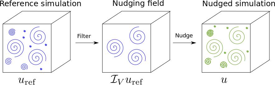
Figure 1: Diagram showing the set-up of our numerical experiments. First, a reference simulation is performed (left). Second, a subset of data is filtered out of the reference field, by keeping only data on a given sub-set of points in space and instant in times (center). Third, we interpolate in time the input partial information and use it to nudge the evolution of a new field to reconstruct the missing data and to infer the correct physics parameters (right).

The nudging technique

As said, nudging means to gently convince a numerical flow to evolve as close as possible to a reference set supposing to have only partial measurements or observations of the latter Waldron et al. (1996); von Storch et al. (2000); Miguez-Macho et al. (2004). The idea is to use the equation of motion to perform an optimal data and flow-parameter assimilation in the interval of time $t\in(0,t^{\prime})$ and in the whole fluid volume. Suppose we have a reference three dimensional turbulent flow, ${\bf u}_{\mathrm{ref}}({\bf x},t)$ evolving under the action of a set of external forces, ${\bf{\cal F}}[{\bf u}_{\mathrm{ref}},{\cal V}_{\mathrm{ref}}]$, parametrised by a set of physical coefficients, ${\cal V}_{\mathrm{ref}}=(\Omega_{\mathrm{ref}},{\cal S}_{\mathrm{ref}},\ell_{\mathrm{ref}},\Delta T_{\mathrm{ref}},\cdots)$ where we denoted with $\Omega_{\mathrm{ref}}$ the rotation rate, with ${\cal S}_{\mathrm{ref}}$ the amplitude of a large scale shear with the typical length scale $\ell_{\mathrm{ref}}$, with $\Delta T_{\mathrm{ref}}$ the temperature difference across the volume etc… Suppose that we have access to the measurements of the reference velocity field, ${\bf u}_{\mathrm{ref}}$ on a limited set of $M$ anemometers placed in ${\bf x}_{j}$ with $j=1,\cdots,M$ that record the flow properties at $N$ time instants $t_{n}$ with $n=1,\cdots,N$ , i.e. we control ${\bf u}_{\mathrm{ref}}$ in a given sub-domain of the whole space-time (3+1) volume only. The idea behind nudging is to evolve an independent three dimensional incompressible Navier-Stokes (NS) equations with an initially educated guess for the set of parameters, ${\cal V}$, and imposing a penalisation whenever the flow field does not reproduce the inputted velocity values of the reference field in the space-time domain $V=({\bf x}_{j},t_{n})$:

$$\frac{\partial{\bm{u}}}{\partial t}+{\bm{u}}\cdot{\bm{\nabla}}{\bm{u}}=-{\bm{\nabla}}p+\nu\nabla^{2}{\bm{u}}+{\bf{\cal F}}[{\bf u},{\cal V}]-\alpha\mathcal{I}_{V}({\bm{u}}-{\bm{u}}_{\mathrm{ref}})$$ (1)

where $\nu$ is the viscosity, $p$ is the pressure that ensures the incompressibility condition, $\mathcal{I}_{V}$ is a dimensionless linear projector operator given by the characteristic function of the set ${V}$, and $\alpha$ is a parameter that controls the intensity imposed by the nudging control and has units of frequency. In its crudest form, $\mathcal{I}_{V}$ is equal to 1 for $({\bf x},t)\in V$ and 0 otherwise. The simplest and most common improvement is to linearly interpolate the different measured snapshots between each time $t_{n}$ and $t_{n+1}$. So when entering (1), ${\bf u}_{\mathrm{ref}}$ will always be assumed to be piece-wise differentiable in time with a characteristic interpolation window, $\tau$. In this way the operator $\mathcal{I}_{V}$ is only acting on the spatial part of the fields. The whole protocol is sketched in Fig. 1. It is important to realize that, in our application, we do not even require to know the exact way the system is forced, i.e. we do not impose ${\cal V}={\cal V}_{\mathrm{ref}}$ and the only a priori information that we provide is inside the partial measurements of the reference field. Clearly, the success of the reconstruction will depend on the amount of information provided (how many measurements in space and in time), on its quality (where and what we measure) and on the intensity of the penalization term, $\alpha$. Notice that, because of potential stiffness and truncation effects arising when $\alpha$ is big, it is not a priori obvious that taking large $\alpha$ is the best choice. It is intuitive to imagine that in some cases it might be better to allow for a larger error in some measuring stations to allow the field to be closer to the target globally.

Set-up of the numerical spectral nudging experiment

We start first by restricting to the case when the set of external parameters are given by the intensity of the Coriolis force due to the presence of a rotation $\Omega$ in the vertical direction and of an external stirring mechanism $\bm{{\cal S}}$:

$${\bf{\cal F}}[{\bf u},{\cal V}]=2\Omega\,\hat{{\bf z}}\times{\bf u}({\bf x},t)+\bm{{\cal S}}({\bf x}).$$ (2)

where $\bm{{\cal S}}$ is a randomly-generated, quenched in time, isotropic field with support on wavenumbers with amplitudes $k\in[k_{f1},k_{f2}]$ whose Fourier coefficients are given by $\bm{\hat{{\cal S}}}({\bf k})=\mathcal{S}k^{-7/2}e^{i\theta_{\bf k}}$, where $\theta_{\bf k}$ are the random phases. In the remaining part of this paper we will address the most ideal case when the information is supplied in Fourier space, i.e. we imagine to have a periodic array of measurement stations that allow us to reconstruct the reference flow configuration in a given range of nudged wavenumbers, $k_{0}<k<k_{1}$. In this case, the $\mathcal{I}_{V}$ operator reduces to a band-pass Fourier filter of the form

$${\cal I}_{V}{\bf u}=\sum_{k_{0}<|{\bf k}|<k_{1}}{\hat{\bf u}}({\bf k},t)\exp{(i{\bf k}\cdot{\bf x})},$$ (3)

that projects the velocity field on the window of nudged Fourier modes.

We implement the whole protocol as follows. First we numerically produce a full space-time evolution of the whole ${\bf u}_{\mathrm{ref}}$ field in a interval $t\in(0,T_{tot})$ by solving the Navier-Stokes equations with a reference rotation rate $\Omega_{\mathrm{ref}}$ and a given intensity of the shear ${\cal S}_{\mathrm{ref}}$ (i.e., Eqs (1) with $\alpha=0$). The values of $\Omega_{\mathrm{ref}}$ and ${\cal S}_{\mathrm{ref}}$ (and also $\nu$ which is the same for both the reference and the nudged simulations) are given in Table 1. All reference simulations are started from rest and allowed to reach stationary states ($t=0$ denotes the start of the stationary states). Second, we extract the inputting field in a subset of discrete times $t_{n}=n\tau$ with $\tau$ chosen as a fraction of the characteristic eddy turnover time of the flow (see Table 1) . Third, we define the nudging field (3) by a linear interpolation between $t_{n}$ and $t_{n+1}$ for all intervals. The initial condition used for all nudged simulation is just the first extracted input field (i.e., the field at $t=t_{0}$) with all the modes outside the nudging region filtered out. All simulations have been performed with a parallel pseudo-spectral code. The code uses a two step Adams Bashfort scheme for the time integration, the “2/3 rule” for dealiasing and periodic boundary conditions in all three directions. In the following we will analyze three different nudging protocols. The first two cases are about simulations made to infer the physical flow parameters, $\Omega_{\mathrm{ref}}$ and $\mathcal{S}_{\mathrm{ref}}$ (called INFER1 and INFER2 in the following, see also Table I for details). The third case is about the reconstruction of the large-scale coherent structures and it is called PHYS1. Numerical details for all set-ups can be found in Table 1. The value of $\tau$ is such that it is smaller than the decorrelation time of the fastest nudged mode, while $\alpha$ was taken as $1/\tau$, these choices follow common practices Omrani et al. (2012). A comprehensive report about the performance of nudging at changing $\alpha,\tau$ for fully developed homogeneous and isotropic turbulent flow is not the scope of this paper and it will be presented elsewhere.

Set-up	$E_{kin}$	$T$	$\nu$	$\mathrm{Re}$	$\mathcal{S}_{\mathrm{ref}}$	$[k_{f1},k_{f2}]$	$\Omega_{\mathrm{ref}}$	$[k_{0},k_{1}]$
INFER1	1.84	3.28	0.002	6030	0.005	[1,2]	2	$[1,4]$
INFER2	1.20	4.06	0.0025	4900	0.02	[1,2]	0	$[1,4]$
PHYS1	0.0012	128	0.002	150	0.004	[10,11]	20	$[8,20]$

Table 1: Parameters used in the different numerical experiments. INFER1 is the set-up for the $\Omega$ scan, INFER2 for the $\mathcal{S}$ scan, and PHYS1 for the inverse cascade experiment. The values listed are the total kinetic energy $E_{kin}=1/2\langle|{\bf u}|^{2}\rangle$, the eddy turnover time $T=L/(2E_{kin})^{1/2}$, with $L=2\pi$ being the largest scale in the flow (same for all simulations), the viscosity $\nu$, the Reynolds number $\mathrm{Re}=L(2E_{kin})^{1/2}/\nu$, the forcing intensity of the reference simulation $\mathcal{S}_{\mathrm{ref}}$, the band of forced wavenumbers in the reference simulation $[k_{f1},k_{f2}]$, the rotation frequency of the reference simulation $\Omega_{\mathrm{ref}}$, and the band of nudged wavenumbers $[k_{0},k_{1}]$. The number of grid points $N^{3}_{\mathrm{grid}}=256^{3}$, the time step of the simulations $dt=0.001$, the nudging intensity $\alpha=10$, and the temporal interpolation window of the nudging field $\tau=0.1$ are the same for all simulations. The box length $L$, the temporal timestep $dt$, the resolution $N^{3}_{\mathrm{grid}}$, and the viscosity $\nu$ are the same for the reference and the nudged simulations in each set. The kinetic energy and Reynolds numbers are given for the reference run of each set, the nudged ones have very similar values.

Inferring physical parameters in rotating turbulence

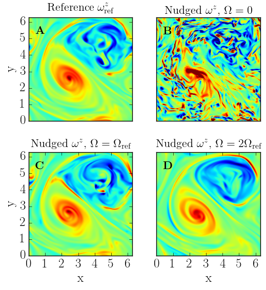
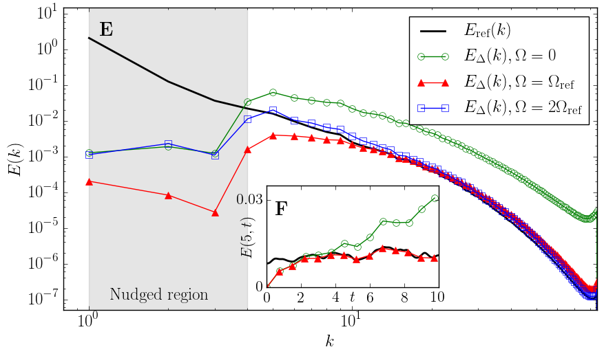
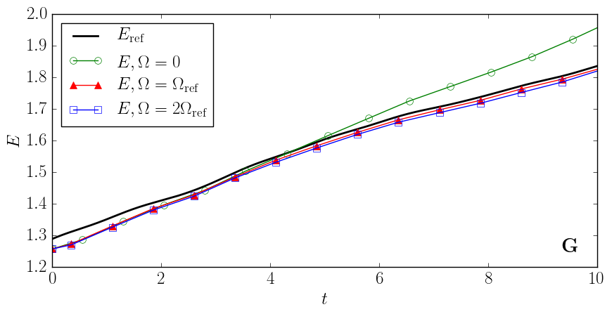
Figure 2: Nudging with different rotation rates. Simulations from set-up INFER1 (see Table 1). A-D: 2D slices of the vorticity field, $\bm{\omega}=\nabla\times{\bf u}$, in the direction parallel to the rotation axis for the reference simulation with a rotation frequency $\Omega_{\mathrm{ref}}$, and three nudged simulations performed with $\Omega=0,\Omega_{\mathrm{ref}},$ and $2\Omega_{\mathrm{ref}}$, respectively. E: Energy spectra of the reference simulation compared with error spectra $E_{\Delta}(k)$ (see Eq. (4)) for different values of the rotation frequency $\Omega$. All spectra were computed at the same instants of time. The shaded gray area indicate the modes where the nudging is acting. F: Time evolution of $E(k,t)$ for $k=5$ for $\Omega=\Omega_{\mathrm{ref}}$ and $\Omega=0$, compared to the reference data. G: Evolution of total energy for the reference field and for the three nudged simulations at changing $\Omega$.

We start by asking how to guess the exact value of the rotation rate, $\Omega_{\mathrm{ref}}$, without any a priori knowledge on its value. To give a first idea on the applications of nudging, in panels (A-D) of Fig. 2 we show a series of 2D slices of the vorticity field in the direction parallel to the rotation axis for the reference simulation (panel A) and for three different nudged simulations (panels B-C-D), two with wrong rotation rates, $\Omega=0$ and $\Omega=2\Omega_{\mathrm{ref}}$, and one with the correct value, $\Omega=\Omega_{\mathrm{ref}}$. Furthermore, in this set of simulations we took ${\cal S}=0$, i.e. we suppose to not know the forcing mechanism (all simulations are from set-up INFER1 shown in Table 1). All snapshots were taken at the same instant in time. Comparing the four panels, it is clear that the simulation nudged with the correct rotation rate (panel C) does reconstruct the reference flow (panel A) much better then the other two (panels B and D). It is also worth pointing out that the standard deviation of the vorticity fields is recovered when rotation is present, with the values begin around $2.8$ for the reference and the simulations of both panels C and D, but this is not the case in the absence of ration (panel C), where the standard deviation takes a value around $5.4$. All fields have zero mean by construction. These qualitative results already provide a first glance of the two main points we make: (i) spectral nudging does work well also for fully turbulent 3D flows, as it does reproduce non-trivial features with high accuracy and (ii) by optimizing the reconstruction properties, one can infer the unknown flow-parameters of the nudging flow. It is worth noticing that the percentage of nudged modes is very small, of the order of $\#_{nudged}\sim 1\times 10^{-4}$, as we are nudging up to $k=4$ while the maximum possible wavenumber in this simulation is $k=85$. The nudged modes are the ones containing the largest amount of energy, but the flow is not completely determined by their evolution, as many more scales should be controlled in order to achieve this Lalescu et al. (2013). This fact is clear when looking at the error spectra in Fig. 2, the error in the unnudged scales is of the order of the energy at that scales even though the large scale reconstruction is very good, meaning the unnudged scales are not slaved to the energy containing modes. Some synchronization of the small scales is nonetheless present, specially for the case with $\Omega=\Omega_{\mathrm{ref}}$. Understanding how much one needs to nudge in order to fully control a turbulent flow is an open question that will be addressed in future work.

In order to control the performance of the nudging protocol in quantitative terms and scale by scale, we introduce a field given by the difference among the exact input and the one reconstructed via (1), $\Delta{\bf u}={\bf u}-{\bf u}_{\mathrm{ref}}$, and we study its spectral properties:

$$E_{\Delta}(k,t)=\frac{1}{2}\sum_{k\leq|{\bf k}|<k+1}|\hat{{\bm{u}}}({\bf k},t)-\hat{{\bm{u}}}_{\mathrm{ref}}({\bf k},t)|^{2}.$$ (4)

Clearly, the smaller the spectrum $E_{\Delta}(k)$, the better the reconstruction. This spectrum will be referred to as the error spectrum.

In the bottom panel (E) of Fig. 2 we show three different curves for $E_{\Delta}(k,t)$ obtained by averaging over all times when we provide the information, $t_{n}$, and for the three different values of the rotation rate, $\Omega=0,\Omega_{\mathrm{ref}},2\Omega_{\mathrm{ref}}$ already discussed in panels (A-D), together with the spectrum of the reference field $E_{\mathrm{ref}}(k)=\sum_{k\leq|{\bf k}|<k+1}|\hat{{\bm{u}}}_{\mathrm{ref}}({\bf k},t)|^{2}$, averaged on the same set of times. In the figure, the set of nudged wavenumbers is denoted by the grey area. From panel (E) it is clear that the optimal nudging is obtained when $\Omega=\Omega_{\mathrm{ref}}$ is used in (1), as revealed from the scale-by-scale nudging error, $E_{\Delta}(k)$, that becomes much smaller than $E_{\mathrm{ref}}(k)$ for $k\in(k_{0},k_{1})$. In all cases, there is a dip in the error spectra at $k=3$, as this is the first scale at which the forcing is not present in the reference flow, so the nudging is able to do a better job reconstructing the data. At $k=4$ the error spectra increases again, mainly because some unnudged modes are integrated when calculating the spectra at this wavenumber. For $\Omega=\Omega_{\mathrm{ref}}$, the scale-by-scale error stays smaller than the reference spectrum up to $k\sim 10$ suggesting a good ability for data assimilation outside the set of nudged degrees of freedom also. This latter fact is also confirmed by the inset (panel F) where we show the temporal evolution of $E_{\mathrm{ref}}(k,t)$ for an unnudged wavenumber, $k=5$, compared with the spectra of the reconstructed field evolved with $\Omega=0$ and $\Omega=\Omega_{\mathrm{ref}}$. In this experiment we started the nudged simulations from zero velocity. As one can see, after a short transient, only the field evolved with the correct $\Omega$ rate is indeed able to synchronize with the time evolution of the inputting data. Finally, we also show the evolution of the total energy in panel G for the same simulations. While the case with $\Omega=0$ is easy to pick apart, the other two are very close to tell which is one produces a better reconstruction of the flow. This indicates that comparing averaged quantities (such as the total energy) may not be the most precise way to determine the value of a parameter.

To be more quantitative about the sensitivity to infer the unknown rotation rate, we have performed also a detailed scan of $\Omega$ values around $\Omega_{\mathrm{ref}}$. In Fig. 3A we show the performance of the nudging reconstruction by plotting the value of the spectrum $E_{\Delta}(k)$, as a function of $\Omega$ and averaged in time and in the nudged window:

$$C=\frac{1}{N\,K}\sum_{n=1}^{N}\int_{k_{0}}^{k_{1}}dkE_{\Delta}(k,t_{n}),$$ (5)

where $t_{n}$ are the instant in times where we have measurements and $K=\int_{k_{0}}^{k_{1}}dkE_{\mathrm{ref}}(k)$ is a normalization factor. Notice that $C$ is defined using information of the nudging data only, i.e. the filtered reference field at the specific times when the information is provided. In contrast, $E_{\Delta}(k)$ needs the whole ${\bf u}_{\mathrm{ref}}$ which in most practical applications would not be available, but that we can nevertheless access in our numerical experiment.

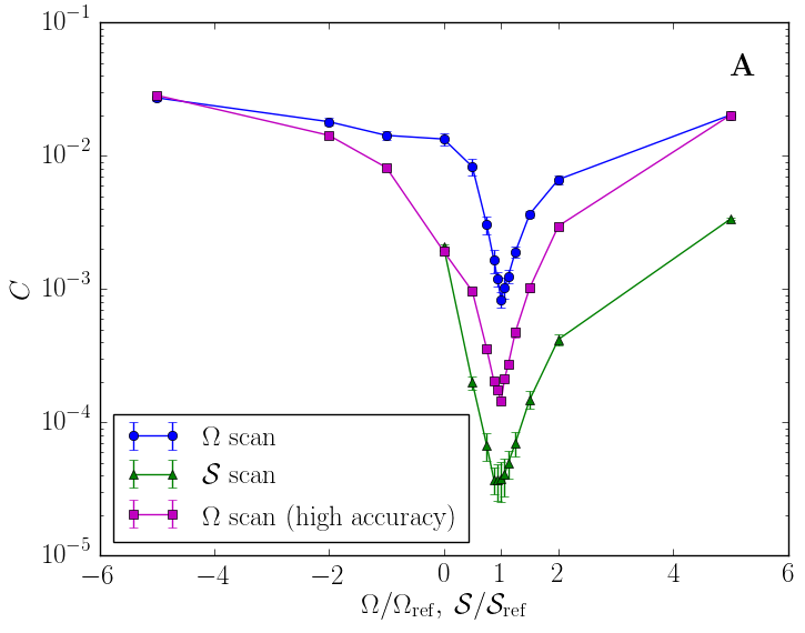
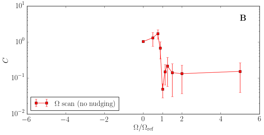
Figure 3: A: Value of the mean error committed to reconstruct the reference field in the nudged window, ${C}$, for two different scanning of the phase space parameters. Blue circle: the case with fixed stirring mechanism and at changing the rotation rate $\Omega$ (set-up INFER1 in Table 1). Green triangles: the case with fixed rotation rate and at changing the intensity of the stirring parameter, $\mathcal{S}$ (set-up INFER2 in Table 1). Magenta squares: a further scan for $\Omega$ following INFER1 but nudging all wavenumbers up to $k=10$. In all cases a clear deep is measured only when the scanning values do correspond to the ones used for the reference data, $\Omega_{\mathrm{ref}}$ and $\mathcal{S}_{\mathrm{ref}}$ respectively. Error bars for each data point were calculated by measuring the standard deviation of $C$. B: Scan of $\Omega$ perfomed without nudging but adding the forcing term (i.e., same as INFER1 but with $\alpha=0$ and $\mathcal{S}=\mathcal{S}_{\mathrm{ref}}$).

From Fig. 3A, it is clear the existence of a minimum in the error when evolving (1) with $\Omega\sim\Omega_{\mathrm{ref}}$. Furthermore, we can determine the correct value of $\Omega$ with a $6.25\%$ error. The error is calculated by looking at which values the errorbars for $C$ overlap. We performed another experiment (set-up INFER2 in Table 1) to test if the intensity $\mathcal{S}$ of mechanical forcing of the reference simulation could also be discovered with our nudging protocol. In this experiment a new reference simulation with $\Omega_{\mathrm{ref}}=0$ and $\mathcal{S}_{\mathrm{ref}}=0.02$ was produced and used to extract the nudging fields (see Table 1 for details). In Fig. 3A we show that the protocol is able to infer the intensity of the stirring mechanism also, with a clear minimum of the error (5) in the proximity of ${\cal S}\sim{\cal S}_{\mathrm{ref}}$. In this case, the correct value of ${\cal S}$ can be pinpointed with a $12.5\%$ error. A third experiment, following INFER1 but nudging more wavenumbers (so using more information from the reference as well is shown. Here all wavenumbers up to $k=10$ where nudged. By doing this we can reduce the error in the estimation of $\Omega$ to $3.125\%$. All numerical experiments show that spectral nudging can be used in a physics-informed way to fit parameters to data and, thus, extract information from it. Furthermore, in set-up INFER1, where no information about the external stirring mechanism is used, performing a one-dimensional scan (i.e. varying only the rotation rate) works well. Having said this, we cannot conclude that this must be the case for generic search in a multi-dimensional phase-space, where the only systematic way to proceed would be to adopt a local gradient-descent algorithm.

A similar scan was performed for the rotation rate but without using the nudging (i.e., $\alpha=0$). In this case, the forcing term was also added (with $\mathcal{S}=\mathcal{S}_{\mathrm{ref}}$), otherwise there would be no energy injection mechanism present. All other parameters are the same as set-up INFER1. The results are shown in Fig. 3B. It is clear that obtaining an accurate value of $\Omega$ out of this scan is very difficult because even though a minimum is readily seen, the errorbars of several datapoints close to it overlap. So while running simulations with different parameter values and performing posterior analysis in order to infer the desired information is possible, our results suggest the using nudging greatly improves the sensitivity and accuracy of the search.

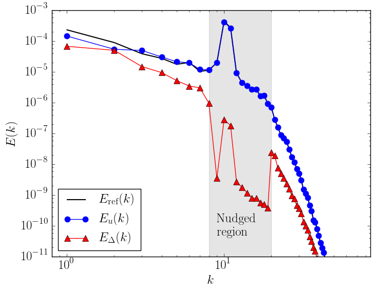
Figure 4: Nudging for the case of rotating turbulence in the inverse energy cascade regime. Simulations from set-up PHYS1 (see Table 1). The nudged window is given by the grey area between $k_{0}=8$ and $k_{1}=20$. The reference spectrum $E_{\mathrm{ref}}$ and the nudged spectrum $E_{u}$ almost coincide for $k>8$, making it hard to discern between the two. Both the intensity of the forcing $\mathcal{S}$ and the rotation rate $\Omega$ are zero in the nudged simulation, so all energy injection and anisotropic effects are coming from the nudging term. Notice the strongly reduced error spectrum $E_{\Delta}(k)$ for a large set of wavenumbers, indicating an optimal reconstruction quality.

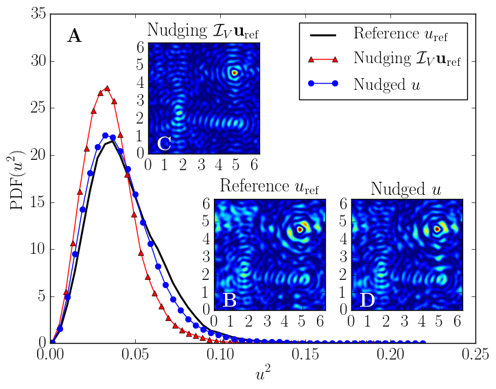
Figure 5: A: Probability density functions (PDF) of the point-wise kinetic energy for the reference simulation $|{\bf u}_{\mathrm{ref}}({\bf x})|^{2}$ (continuous black line), the nudged simulation $|{\bf u}({\bf x})|^{2}$ (circles) and the nudging input field $|\mathcal{I}_{V}{\bf u}_{\mathrm{ref}}({\bf x})|^{2}$ (triangles) for the inverse cascade experiment (set-up PHYS1 in Table 1). B-D: 2D slices of planes perpendicular to the rotation axis of the absolute velocity fields.

Inferring the large-scale velocity distribution without input rotation

In this section we describe how to use nudging to infer, under some circumstances, the entire set of large-scale physical flow structures of the reference data without a detailed knowledge of the forces acting on flow. To test this idea we performed a new experiment by using a turbulent flow under rotation and in the presence of an inverse energy cascade. It is well known that if rotation is strong enough and energy is injected at large wavenumbers the flow undergoes a transition from a direct to a split turbulent energy cascade, accumulating kinetic energy and producing a non-trivial cyclonic distribution of vortices at larger and larger scales Smith et al. (1996); Mininni and Pouquet (2009); Mininni et al. (2009). This regime does not occur naturally in homogeneous isotropic three-dimensional turbulence Biferale et al. (2013), but it is argued to be important in many geophysical set-ups in the oceans Scott and Wang (2005); Corrado et al. (2017) and in the atmosphere Lacorata et al. (2004). Here, we show how a suitable nudging strategy is indeed able to reconstruct the inverse energy cascade even in the absence of any explicit rotation term in the nudged equations (1), provided that the ${\bf u}_{\mathrm{ref}}$ is inputting information around the injection scale. To do this we use a rotating turbulent flow forced at $k_{f}=10$ and with $\Omega_{\mathrm{ref}}=20$ and $\mathcal{S}_{\mathrm{ref}}=0.004$ as a reference (set-up PHYS1 in Table 1) where an inverse energy cascade develops. We then evolve (1) without any rotation and any external forcing:

$${\bf{\cal F}}[{\bf u}_{\mathrm{ref}},{\cal V}_{\mathrm{ref}}]=0$$

in this way we are completely ignorant about the physics we want to reproduce. In Fig. 4 we show that by nudging in the region around the injection mechanism, the energy spectra of the reference simulation is well reproduced by the nudged simulation even, and in particular, in the inverse energy cascade range. The presence of a strong peak around the forced wavenumber is typical of systems where an inverse cascade is present, as this is a slow and inefficient transfer mechanism Smith et al. (1996); Mininni and Pouquet (2009); Mininni et al. (2009); Biferale et al. (2016). Even though the only information we input is the nudging filtered field, the nudged evolution is able to reconstruct the inverse cascade and the correct spectrum slope even for scales much smaller then the ones where we nudge. It is remarkable how the spectrum error, $E_{\Delta}(k)$ is small also for modes outside the nudging window $k<k_{0}$ and $k>k_{1}$, indicating the presence of strong non-local spectral correlation in the split-energy cascade mechanism which are fully reconstructed by our protocol.

To go beyond spectral properties and to check the ability to reconstruct the large-scale coherent structures in the rotating flow, we plot in Fig. 5 the probability density functions (PDFs) of the space-dependent kinetic energy for the reference simulation, $|{\bf u}_{\mathrm{ref}}|^{2}/2$, the nudged simulation, $|{\bf u}|^{2}/2$, and the nudging field, $|\mathcal{I}_{V}{\bf u}_{\mathrm{ref}}|^{2}/2$. As one can see, the reconstructed field has a PDF very close to the reference case, even if the nudging input field does not. In the same figure, we also show 2D slices of the absolute velocity fields in planes perpendicular to the rotation axis for the three fields as before. As one can see, the nudged simulation (panel D) is able to extrapolate the unknown large-scale reference flow structures extremely well (panel B), for a case where the nudged inputting data do not contain any information about those scale (C). The apparent patterns seen in these visualizations are a product of the strong forcing present in the system acting around $k=10$.

Conclusions

Spectral nudging is a physics-informed technique commonly used to guide the evolution of chaotic dynamical systems inputting measured data. Giving examples for both isotropic and rotating 3D turbulence, we have shown how this technique can be efficiently used to infer both the physical parameters entering in the external stirring forces and the large-scale velocity distribution for the inverse energy cascade regime, typical of strongly rotating turbulent flows. The method can be further improved and optimised by using different nudging parameters for different degrees of freedoms, e.g. by changing $\alpha$ and $\tau$ with ${\bf k}$. A detailed study of nudging performances for homogeneous and isotropic turbulence at different Reynolds numbers, different nudging windows and at changing the spatial locations of the measurements stations will be reported elsewhere.

Other strategies used to estimate parameters, such as variational methods Navon (1998) or ensemble based methods Anderson and Anderson (1999); Anderson (2001); Ruiz et al. (2013), require the need to postulate and error correlation matrix and make assumptions about the behavior of the errors and deviations, need to use linearized models (for variational methods), or are based on minimizing complicated functions (again for variational methods). Nudging based strategies do require to perform several forwards simulations, similar to ensemble based method. One advantage other methods have compared to nudging, is the ease to incorporate information on observables (such as precipitation, for example) and not just state variables (such as the velocity field, as was used here. Interestingly, variational data assimilation schemes have been exploited to determine vectors of optimal nudging coefficients Zou et al. (1992). Here, we reversed the point of view: given the coefficients $\alpha,\tau$, we employed nudging to estimate the physical flow parameters. Finally, the method is also general and extendable to other problems, opening the route to applications for parameter inferring to a vast set of hydrodynamical situations including, to cite just the most promising cases, i) optimising sub-grid-scale models in Large Eddy Simulations, by inferring parameters against data extracted from either observation or benchmark direct numerical simulations; ii) large-scale turbulent transport to determine eddy-viscosity and eddy-diffusivity Yu and O’Brien (1991); Lin et al. (2001); iii) the identification of ambient air sources and the quantification of their contribution to pollution levels (the so-called source apportionment problem) Bove et al. (2014); iv) partial field reconstruction using advanced Lidar systems Cooper et al. (1997) to reveal the free parameters characterizing the atmospheric boundary layer; v) correction of velocity fields in ocean circulation models with Lagrangian data (e.g. from drifting buoys) Taillandier et al. (2006a, b) and/or other sources including HF radar data Berta et al. (2014).