Theory of tunneling spectroscopy of normal metal/ferromagnet/spin-triplet superconductor junctions

Abstract

We study the tunneling conductance of a ballistic normal metal / ferromagnet / spin-triplet superconductor junction using the extended Blonder-Tinkham-Klapwijk formalism as a model for a $c$-axis oriented Au / SrRuO₃ / Sr₂RuO₄ junction. We compare chiral $p$-wave (CPW) and helical $p$-wave (HPW) pair potentials, combined with ferromagnet magnetization directions parallel and perpendicular to the interface. For fixed $\theta_{M}$, where $\theta_{M}$ is a direction of magnetization in the ferromagnet measured from the $c$-axis, the tunneling conductance of CPW and HPW clearly show different voltage dependencies. It is found that the cases where the $d$-vector is perpendicular to the magnetization direction (CPW with $\theta_{M}=\pi/2$ and HPW with $\theta_{M}=0$) are identical. The obtained results serve as a guide to determine the pairing symmetry of the spin-triplet superconductor Sr₂RuO₄.

I Introduction

Nowadays, Sr₂RuO₄ is known as an unconventional superconductor with the transition temperature $T_{c}\sim 1.5$ K. Maeno et al. (1994) The fact that the Knight shift does not change across $T_{c}$ is consistent with spin-triplet pairing.Ishida et al. (1998); Tou et al. (1998); Murakawa et al. (2004); Mackenzie and Maeno (2003); Maeno et al. (2012) Various theoretical studies have discussed the microscopic mechanism of spin-triplet pairings in this material. Rice and Sigrist (1995); Miyake and Narikiyo (1999); Kuwabara and Ogata (2000); Nomura and Yamada (2000, 2002a, 2002b); Arita et al. (2004); Nomura and Yamada (2005); Nomura et al. (2008); Yanase and Ogata (2003); Raghu et al. (2010); Sato and Kohmoto ; Kuroki et al. (2001); Takimoto (2000); Tsuchiizu et al. (2015) The existence of a zero bias conductance peak in several tunneling experiments Laube et al. (2000); Mao et al. (2001) indicates the realization of unconventional superconductivity. Tanaka and Kashiwaya (1995); Kashiwaya and Tanaka (2000); Yamashiro et al. (1997) In particular, the broad zero bias conductance peak observed in tunneling spectroscopy suggests the realization of a surface Andreev bound states (SABS) with linear dispersion Kashiwaya et al. (2011); Yamashiro et al. (1997, 1998); Honerkamp and Sigrist (1998). This is in contrast with high $T_{c}$ cuprate superconductors, where a sharp zero bias conductance peak is observed Kashiwaya and Tanaka (2000); Tanaka and Kashiwaya (1995); Kashiwaya et al. (1995, 1998); Covington et al. (1997); Alff et al. (1997); Wei et al. (1998); Iguchi et al. (2000) due to flat band zero energy states.Tanaka and Kashiwaya (1995); Hu (1994); Sato et al. (2011) When spin-triplet pairing is realized, we can expect exotic phenomena, such as the so called anomalous proximity effect in diffusive normal metal / spin-triplet superconductor junctions. Tanaka and Kashiwaya (2004); Tanaka et al. (2005a); Asano et al. (2006); Tanaka et al. (2005b); Asano et al. (2011)

The presence or absence of time reversal symmetry (TRS) in Sr₂RuO₄ is an important issue. Among two-dimensional spin-triplet $p$-wave pairings, chiral and helical $p$-wave pairing seem promising in the absence and presence of TRS, respectively.Qi and Zhang (2011) Broken TRS was observed in $\mu$SR and Kerr-rotation experiments as a result of a spontaneous internal magnetic field below $T_{c}$,Luke et al. ; Xia et al. (2006a); Matsumoto and Sigrist (1999); Xia et al. (2006b) which supports chiral $p$-wave pairing. However, the internal magnetic field has not been detected in scanning SQUID experiments,Kirtley et al. (2007); Hicks et al. (2010) which suggests realization of helical $p$-wave symmetry. Although there are several possible explanations for the absence of broken TRS in Sr₂RuO₄, Huang et al. (2014); Lederer et al. (2014); Ashby and Kallin (2009); Huang et al. (2015); Raghu et al. (2010); Bouhon and Sigrist (2014); Tada et al. (2009); Suzuki and Asano (2016) the pairing symmetry remains a point of discussion. One of the main differences between these two pairing symmetries is the direction of $d$-vector.

A constructive way to distinguish between them is to study the charge transport in ferromagnet / spin-triplet superconductor junctions.Hirai et al. (2001, 2003); Yoshida et al. (1999); Li and Yang (2012); Cheng and Jin (2013) Naively speaking, the direction of the magnetization axis with respect to the $d$-vector (parallel or perpendicular) influences the charge transport. Recently, a Au / SrRuO₃ / Sr₂RuO₄ junction oriented along the $c$-axis has been fabricated by means of epitaxial growth.Anwar et al. (2016) Since SrRuO₃ and Sr₂RuO₄ have similar $a$-axis lattice constants, as well as similar atomic arrangements, a smooth interface between them can be expected, which turns this system into a nice playground for clarifying the direction of the $d$-vector. Because the SABS is absent in this direction, we can directly compare the effect of the magnetization direction relative to the $d$-vector. To interpret the experimental results, a theoretical model is required in which we calculate the tunneling conductance along the $c$-axis, based on a minimal model which takes the quasi-two dimensional nature of Sr₂RuO₄ into account.

In this paper, we investigate normal metal (N) / ferromagnet (F) / spin-triplet superconductor (S) junctions with $s$-wave, chiral and helical $p$-wave pairing symmetries by changing the properties of the ferromagnet, $e.g.$, thickness, magnetization strength and direction. The anisotropic Fermi surface of Sr₂RuO₄ and realistic effective masses are also included, since the Fermi-momentum mismatch changes the transparency and the resulting conductance. Finally, an external magnetic field is taken into account through the Doppler shift.

II Formulation

II.1 Model and Hamiltonian

We consider a three-dimensional N/F/S junction, as shown in Fig. 1.

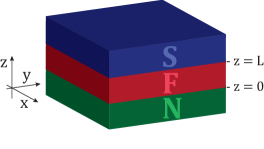
Figure 1: Schematic of the three-dimensional normal metal(N)/ferromagnet(F)/superconductor(S) junction. We assume the structure extends to infinity in all directions.

We assume the junction interfaces to be perpendicular to the $z$-axis and located at $z=0$ and $z=L$. The F has a thickness $L$ and a magnetization $\boldsymbol{M}(z)$. The N and S are considered to be semi-infinite. Superconducting junctions are described by the Bogoliubov-de Gennes (BdG) Hamiltonian

$$\mathcal{\check{H}}(\boldsymbol{r}) =\left[\begin{array}[]{cc}\hat{h}(\boldsymbol{r},H){}&\hat{\Delta}(\boldsymbol{r}){}\\[5.69054pt] -\hat{\Delta}^{*}(\boldsymbol{r}){}&-\hat{h}^{*}(\boldsymbol{r},H){}\\ \end{array}\right],$$ (3)

where the basis is taken as $\Psi(\boldsymbol{r})=[\,\psi_{\uparrow}(\boldsymbol{r})\hskip 5.69054pt\psi_{\downarrow}(\boldsymbol{r})\hskip 5.69054pt\psi_{\uparrow}^{\dagger}(\boldsymbol{r})\hskip 5.69054pt\psi_{\downarrow}^{\dagger}(\boldsymbol{r})\,]^{T},$ where $T$ is the transpose, the symbol $\hat{\cdot}$ ($\check{\cdot}$) represents a $2\times 2$ ($4\times 4$) matrix in the spin (spin-Nambu) space, $H$ is an externally applied magnetic field in the $x$-direction. Since the system has translational symmetry in the $x$- and $y$-direction, the momenta $k_{x}$ and $k_{y}$ are well-defined quantum numbers. Therefore, the wave function can be expressed in the Fourier components as

$$\Psi(\boldsymbol{r})=\sum_{\boldsymbol{k}_{\parallel}}\Psi_{\boldsymbol{k}_{\parallel}}(z)\frac{e^{i(k_{x}x+k_{y}y)}}{\sqrt{L_{x}L_{y}}},$$ (4)

$$\Psi_{\boldsymbol{k}_{\parallel}}(z)=[~{}\psi_{\uparrow,{\boldsymbol{k}_{\parallel}}}~{}~{}\psi_{\downarrow,{\boldsymbol{k}_{\parallel}}}~{}~{}\psi_{\uparrow,{-\boldsymbol{k}_{\parallel}}}^{\dagger}~{}~{}\psi_{\downarrow,{-\boldsymbol{k}_{\parallel}}}^{\dagger}~{}]^{T},$$ (5)

where $\boldsymbol{k}_{\parallel}=(k_{x},k_{y},0)$. In Eq. (4), we assume periodic boundary conditions in order to accommodate the infinite dimensions in the $x$- and $y$-direction. The lateral dimensions $L_{x}$ and $L_{y}$ are normalization factors and do not affect the conductance spectrum. The Hamiltonian becomes

$$\mathcal{\check{H}}_{\boldsymbol{k}_{\parallel}}(z,H) =\left[\begin{array}[]{cc}\hat{h}_{\boldsymbol{k}_{\parallel}}(z,H){}&\hat{\Delta}_{\boldsymbol{k}_{\parallel}}(z){}\\[5.69054pt] -\hat{\Delta}^{*}_{-\boldsymbol{k}_{\parallel}}(z){}&-\hat{h}^{*}_{-\boldsymbol{k}_{\parallel}}(z,H){}\\ \end{array}\right].$$ (8)

The single-particle Hamiltonian $\hat{h}_{\boldsymbol{k}_{\parallel}}$ is given by

$$\hat{h}_{\boldsymbol{k}_{\parallel}}(z,H)=\xi_{\boldsymbol{k}_{\parallel}}(z,H)+\boldsymbol{M}(z)\cdot\boldsymbol{\hat{\sigma}}+\hat{F}_{\boldsymbol{k}_{\parallel}}(z),$$ (9)

$$\xi_{\boldsymbol{k}_{\parallel}}(z,H)=-\frac{\hbar^{2}}{2m_{z}}\frac{\partial^{2}}{\partial z^{2}}-\mu^{\prime}-\Delta_{0}\frac{H}{H_{c}}\frac{k_{\parallel}}{k_{F}}\sin\varphi,$$ (10)

$$\mu^{\prime}=\mu-\frac{\hbar^{2}}{2}\left[\frac{k_{x}^{2}}{m_{x}}+\frac{k_{y}^{2}}{m_{y}}\right],$$ (11)

where $\xi_{\boldsymbol{k}}$ is the kinetic energy in the presence of an external magnetic field in the $x$-direction and $\mu$ is the chemical potential, which we assume to be constant across the junction. A full derivation of Eq. (10) is given in Appendix A. The matrices $\hat{\sigma}_{j}$ $(j\in\{x,y,z\})$ and $\hat{\sigma}_{0}$ are the Pauli matrices and the identity matrix in spin space, $\hat{\boldsymbol{\sigma}}=\hat{\sigma}_{x}\boldsymbol{{e}}_{x}+\hat{\sigma}_{y}\boldsymbol{{e}}_{y}+\hat{\sigma}_{z}\boldsymbol{{e}}_{z}$ with $\boldsymbol{e}_{j}$ being the unit vectors in the $j$-direction. We can modify the shape of Fermi surfaces by tuning the effective masses $\boldsymbol{m}=(m_{x},m_{y},m_{z})$ in each region. In this paper, we parametrize $\boldsymbol{m}$ as

$$\boldsymbol{m}(z)=\left\{\begin{array}[]{clc}(\,m_{N},~{}m_{N},~{}m_{N}\,)&\hskip 14.22636pt\text{for}&z\leq 0,\\[2.84526pt] (\,m_{F},~{}m_{F},~{}m_{F}\,)&\hskip 14.22636pt\text{for}&0<z<L,\\[2.84526pt] (\,m_{\parallel},~{}m_{\parallel},~{}m_{\perp}\,)&\hskip 14.22636pt\text{for}&z\geq L.\\ \end{array}\right.$$ (15)

The magnetization is described as Cheng and Jin (2013)

$$\boldsymbol{M}(z)=M_{0}(\sin\theta_{M}\boldsymbol{e}_{x}+\cos\theta_{M}\boldsymbol{e}_{z})\Theta(z)\Theta(L-z),$$ (16)

where $\Theta(z)$ is the Heaviside step function. In this paper, we ignore the re-orientation of the $d$-vector by the magnetization in FGentile et al. (2013); Terrade et al. (2013); Brydon and Manske (2009); Brydon (2009) for simplicity. The effects of the interfaces are described by $\hat{F}_{\boldsymbol{k}_{\parallel}}(z)$ as Wu and Samokhin (2010)

$$\hat{F}_{\boldsymbol{k}_{\parallel}}(z)=\delta(z)\hat{F}_{1}+\delta(z-L)\hat{F}_{2},$$ (17)

$$\hat{F}_{1,\boldsymbol{k}_{\parallel}}=F_{1}\hat{\sigma}_{0},$$ (18)

$$\hat{F}_{2,\boldsymbol{k}_{\parallel}}=F_{\mathrm{SO}}\boldsymbol{e}_{z}\cdot(\hat{\boldsymbol{\sigma}}\times\boldsymbol{k}),$$ (19)

where $F_{1}$ and $F_{\mathrm{SO}}$ represent the strengths of the barrier potential at $z=0$ and the spin-orbit coupling (SOC) at $z=L$, respectively. The SOC term reduces to

$$\boldsymbol{e}_{z}\cdot(\hat{\boldsymbol{\sigma}}\times\boldsymbol{k}) =\hat{\sigma}_{x}k_{y}-\hat{\sigma}_{y}k_{x}$$ (20)

$$=ik_{\parallel}\left[\begin{array}[]{cc}0&e^{-i\varphi}\\ -e^{+i\varphi}&0\\ \end{array}\right],$$ (23)

where $k_{x}=k_{\parallel}\cos\varphi$ and $k_{x}=k_{\parallel}\sin\varphi$ with $k_{\parallel}=(k_{x}^{2}+k_{y}^{2})^{1/2}$. The pair potential is described by

$$\hat{\Delta}_{\boldsymbol{k}_{\parallel}}(z)=\underline{\hat{\Delta}}_{\boldsymbol{k}_{\parallel}}(z)\Theta(z-L).$$ (24)

The momentum dependence of the pair potentials for $s$ -wave (SW), chiral $p$ -wave (CPW), and helical $p$ -wave (HPW) superconductors are written as

$$\underline{\hat{\Delta}}_{\boldsymbol{k}_{\parallel}}(z)=\left\{\begin{array}[]{ll}\Delta_{0}i\hat{\sigma}_{y}&\text{for SW, }\\[5.69054pt] \Delta_{0}[\bar{k}_{x}+i\chi\bar{k}_{y}]\hat{\sigma}_{x}&\text{for CPW, }\\[5.69054pt] \Delta_{0}[\bar{k}_{x}\hat{\sigma}_{0}+i\bar{k}_{y}\hat{\sigma}_{z}]&\text{for HPW, }\\ \end{array}\right.$$ (28)

where $\Delta_{0}$ is a constant which characterizes the amplitude of the pair potential, $\chi$ is so-called the chirality (which can be $\pm 1$), $\bar{k}_{x}=k_{x}/k_{s\parallel}$ with $k_{s\parallel}=\sqrt{2m_{\parallel}\mu^{\prime}}/\hbar$ being the Fermi wavenumber in $k_{x}$-$k_{y}$ plane for S. The assumption that $\Delta_{0}$ is constant implies that we do not take the inverse proximity effect (from F into S) into account, which is a common assumption.Blonder et al. (1982)

II.2 Wave functions

The wave function is obtained by solving the Hamiltonian at an energy $E$ in each region. Throughout this paper, we assume $E\sim\Delta_{0}\ll\mu$. The wave function for $z\leq 0$ is given by

$$\Psi_{k_{\parallel}}(z)=\check{K}^{+}_{N}\vec{i}+\check{K}_{N}^{-}\vec{r},$$ (29)

where $\check{K}^{\pm}_{N}=e^{\pm i\check{\tau}_{z}k_{N}z}$ with $k_{N}=\sqrt{2m_{N}\mu^{\prime}}/\hbar$ and $\check{\tau}_{z}=\mathrm{diag}[\hat{\sigma}_{0},-\hat{\sigma}_{0}]$ being the third Pauli matrix in Nambu space. The vector $\vec{i}$ represents the wave function amplitude of the incident particles which is given by

$$\vec{i}=\left\{\begin{array}[]{cl}\left[~{}1~{}0~{}0~{}0~{}\right]^{T}{}&~{}\text{for an up-spin electron},\\[5.69054pt] \left[~{}0~{}1~{}0~{}0~{}\right]^{T}{}&~{}\text{for a down-spin electron}.\\ \end{array}\right.$$ (32)

The vector $\vec{r}$ describes the wave function amplitude of the reflected particles as

$$\vec{r}=[~{}r^{p}_{\uparrow}~{}~{}r^{p}_{\downarrow}~{}~{}r^{h}_{\uparrow}~{}~{}r^{h}_{\downarrow}~{}]^{T},$$ (33)

where $r^{p}_{\alpha}$ and $r^{h}_{\alpha}$, $\alpha\in\{\uparrow,\downarrow\}$ are the normal and Andreev reflection coefficients, respectively. The wave function for $0<z<L$ is given by

$$\Psi_{\boldsymbol{k}_{\parallel}}(z)=\check{A}\check{K}^{+}_{F}\vec{f}_{P}+\check{A}\check{K}^{-}_{F}\vec{f}_{N},$$ (34)

where $\check{K}_{F}^{\pm}=\mathrm{diag}[\,e^{\pm ik_{F}^{+}z},~{}e^{\pm ik_{F}^{-}z},~{}e^{\pm ik_{F}^{+}z},~{}e^{\pm ik_{F}^{-}z}\,]$ with $k_{F}^{\pm}=\sqrt{2m_{F}(\mu^{\prime}\mp M_{0})}/\hbar$. The matrix $\check{A}=\mathrm{diag}[\hat{A},\hat{A}]$ characterizes the spin structure of the F, where $\hat{A}$ is given by Cheng and Jin (2013)

$$\hat{A}=\left[\begin{array}[]{rr}~{}\cos({\theta_{M}}/{2})&~{}-\sin({\theta_{M}}/{2}){}\\[5.69054pt] ~{}\sin({\theta_{M}}/{2})&~{}\cos({\theta_{M}}/{2}){}\\ \end{array}\right]$$ (37)

The vectors $\vec{f}_{P(N)}$ describe the wave function amplitudes of particles propagating in the positive (negative) $z$-direction. They are defined as

$$\vec{f}_{P}= \,[~{}f^{p}_{\uparrow,P}~{}~{}f^{p}_{\downarrow,P}~{}~{}f^{h}_{\uparrow,P}~{}~{}f^{h}_{\downarrow,P}~{}]^{T},$$ (38)

$$\vec{f}_{N}= \,[~{}f^{p}_{\uparrow,N}~{}~{}f^{p}_{\downarrow,N}~{}~{}f^{h}_{\uparrow,N}~{}~{}f^{h}_{\downarrow,N}~{}]^{T}.$$ (39)

The wave function for $z\geq L$ is given by

$$\Psi_{k_{\parallel}}(z)=\check{U}\check{K}_{S}\vec{t},$$ (40)

where $\check{K}_{S}=\mathrm{diag}[~{}e^{+ik_{S}z},\,~{}e^{+ik_{S}z},\,~{}e^{-ik_{S}z},\,~{}e^{-ik_{S}z}~{}]$ with $k_{S}=\sqrt{2m_{\perp}\mu^{\prime}}/\hbar$. The vector $\vec{t}$ describes the wave function amplitudes of the transmitted particles as

$$\vec{t}= \,[~{}t^{p}_{\uparrow}~{}~{}t^{p}_{\downarrow}~{}~{}t^{h}_{\uparrow}~{}~{}t^{h}_{\downarrow}~{}]^{T}.$$ (41)

The matrix $\check{U}$ describes the amplitude of the wave function in the superconductor as

$$\check{U}=\left[\begin{array}[]{ll}u_{\boldsymbol{k}_{\parallel}}\hat{\sigma}_{0}&~{}v_{\boldsymbol{k}_{\parallel}}\,\hat{D}_{\boldsymbol{k}_{\parallel}}\\[5.69054pt] v_{\boldsymbol{k}_{\parallel}}\,\hat{D}_{\boldsymbol{k}_{\parallel}}^{\dagger}&~{}u_{\boldsymbol{k}_{\parallel}}\hat{\sigma}_{0}\\ \end{array}\right],$$ (44)

$$\hat{D}_{\boldsymbol{k}_{\parallel}}=\hat{\underline{\Delta}}_{\boldsymbol{k}_{\parallel}}/\Delta_{0},$$ (45)

with

$$u_{\boldsymbol{k}_{\parallel}}=\frac{1}{\sqrt{2}}\,\sqrt{1+\frac{\Omega_{\boldsymbol{k}_{\parallel}}}{E}},$$ (46)

$$v_{\boldsymbol{k}_{\parallel}}=\frac{1}{\sqrt{2}}\,\sqrt{1-\frac{\Omega_{\boldsymbol{k}_{\parallel}}}{E}},$$ (47)

$$\Omega_{\boldsymbol{k}_{\parallel}}=\sqrt{E^{2}-|d_{\boldsymbol{k}_{\parallel}}|^{2}},$$ (48)

where $d_{\boldsymbol{k}_{\parallel}}$ is obtained from the relation $d_{\boldsymbol{k}_{\parallel}}\hat{\sigma}_{0}=\hat{\underline{\Delta}}_{\boldsymbol{k}_{\parallel}}\hat{\underline{\Delta}}_{\boldsymbol{k}_{\parallel}}^{\dagger}$.

II.3 Differential conductance

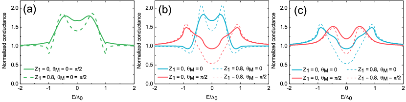
Figure 2: The dimensionless tunneling conductance using pair potentials (a) SW, (b) CPW and (c) HPW. Without barriers ($Z_{1}=0$, solid graphs) and including a small barrier at the first interface ($Z_{1}=0.8$, dashed graphs). The SW case is independent of the magnetization angle. For CPW and HPW, the magnetization angle varies from $\theta_{M}=0$ (blue graphs) to $\theta_{M}=\pi/2$ (red graphs). $X=0.6$, $k_{F}L=11$.

Table 1: Matrix structure of the pair potential. The spin-quantisation axis is taken to be parallel to the magnetisation vector $\boldsymbol{M}$. The first and second rows are for $\boldsymbol{M}\parallel\boldsymbol{z}$ (i.e., $\theta_{M}=0$) and for $\boldsymbol{M}\parallel\boldsymbol{x}$ (i.e., $\theta_{M}=\pi/2$), respectively. From the table, we can see that the $4\times 4$ Hamiltonian can be reduced to two $2\times 2$ Hamiltonian matrices except for the helical $p$ -wave with $\theta_{M}=\pi/2$ case. The angle $\phi$ satisfies the relations: ${k}_{x}=k_{\parallel}\cos\phi$ and ${k}_{y}=k_{\parallel}\sin\phi$ with $k_{\parallel}=|\boldsymbol{k}_{\parallel}|$ being the momentum parallel to the interfaces. The momentum is normalized: $\bar{k}_{x(y)}=k_{x(y)}/k_{\parallel}$. The factor $\chi$ is the chirality of a chiral $p$-wave superconductor.

All coefficients in Eq. (29), (34) and (40) can be determined by the four boundary conditions at $z=0$ and $z=L$. The first two boundary conditions are derived from continuity at $z=0$. They are given byBlonder et al. (1982)

$$\lim_{z\uparrow 0}\Psi_{\boldsymbol{k}_{\parallel}}=\lim_{z\downarrow 0}\Psi_{\boldsymbol{k}_{\parallel}},$$ (49)

$$\lim_{z\uparrow 0}\left[\frac{\partial\Psi_{\boldsymbol{k}_{\parallel}}}{\partial z}+\frac{2m(z)}{\hbar^{2}}\check{F}_{1}\Psi_{\boldsymbol{k}_{\parallel}}\right]=\lim_{z\downarrow 0}\frac{\partial\Psi_{\boldsymbol{k}_{\parallel}}}{\partial z},$$ (50)

where $\check{F}_{1}=\mathrm{diag}[\hat{F}_{1,\boldsymbol{k}_{\parallel}},-\hat{F}_{1,-\boldsymbol{k}_{\parallel}}^{*}]$. The other boundary conditions are related to the interface at $z=L$ as follows

$$\lim_{z\uparrow L}\Psi_{\boldsymbol{k}_{\parallel}}=\lim_{z\downarrow L}\Psi_{\boldsymbol{k}_{\parallel}},$$ (51)

$$\lim_{z\uparrow L}\left[\frac{\partial\Psi_{\boldsymbol{k}_{\parallel}}}{\partial z}+\frac{2m(z)}{\hbar^{2}}\check{F}_{2}\Psi_{\boldsymbol{k}_{\parallel}}\right]=\lim_{z\downarrow L}\frac{\partial\Psi_{\boldsymbol{k}_{\parallel}}}{\partial z},$$ (52)

where $\check{F}_{2}=\mathrm{diag}[\hat{F}_{2,\boldsymbol{k}_{\parallel}},-\hat{F}_{2,-\boldsymbol{k}_{\parallel}}^{*}]$.

In the supplemental material, we derived the expression for the current through the N/F/S junction and found that it was the same as in the original BTK theory.Blonder et al. (1982) Hence, we can use the same differential tunnelling conductance resulting from a spin-$\alpha$ incident particle, which is given by

$${\sigma}(E)=\sum_{\boldsymbol{k}_{\parallel},\alpha}{}^{{}^{\prime}}{\sigma}_{\alpha}(E,\boldsymbol{k}_{\parallel}),$$ (53)

$${\sigma}_{\alpha}(E,\boldsymbol{k}_{\parallel})=1+|r^{h}_{\uparrow}|^{2}+|r^{h}_{\downarrow}|^{2}-|r^{p}_{\uparrow}|^{2}-|r^{p}_{\downarrow}|^{2},$$ (54)

where ${\sigma}_{\alpha}(E,\boldsymbol{k}_{\parallel})$ is the angle-resolved differential conductance for a spin-$\alpha$ incident particle with $\alpha\in\{\uparrow,\,\downarrow\}$.not To model a cylindrical Fermi surface in a quasi-two-dimensional material, we introduce a cutoff in the summation with respect to $\boldsymbol{k}_{\parallel}$ as

$$\sum_{\boldsymbol{k}_{\parallel},\alpha}{}^{{}^{\prime}}\cdots~{}\overset{\mathrm{def}}{=\joinrel=}~{}\sum_{\boldsymbol{k}_{\parallel},\alpha}\cdots\Theta\big{(}|\boldsymbol{k}_{\parallel}|-k_{c}\big{)}$$ (55)

where $k_{c}=k_{N}\sin\theta_{c}$ and $\theta_{c}$ is the cutoff angle.

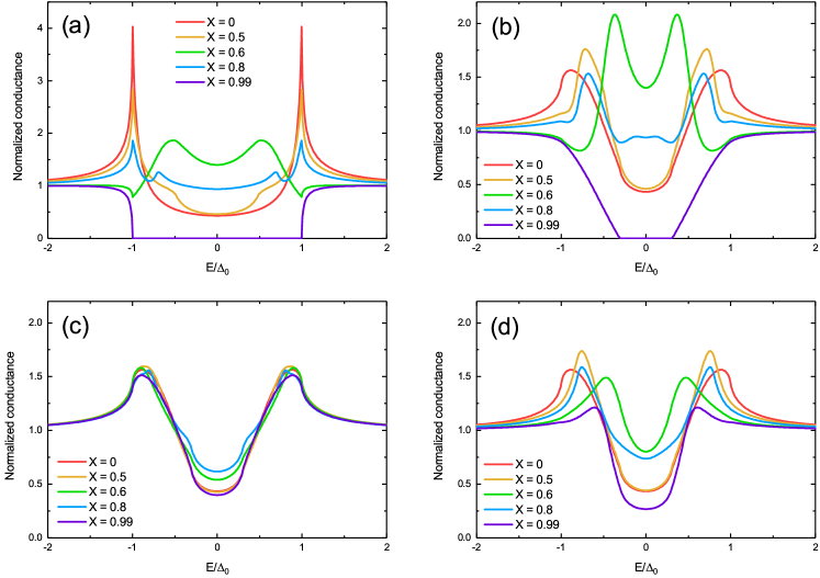
Figure 3: Dimensionless tunneling conductance using pair potentials (a) SW, (b) CPW, $\theta_{M}=0$, (c) HPW, $\theta_{M}=0$ which is identical to CPW, $\theta_{M}=\pi/2$ and (d) HPW, $\theta_{M}=\pi/2$. Magnetization strengths varying from $X=0$ (normal metal) to $X=0.99$ (fully polarized). $Z_{1}=0.8$, $k_{F}L=11$.

III Results

The aim of this paper is to model the conductance of a Au/SrRuO₃/Sr₂RuO₄ junction. A realistic effective mass for ferromagnet SrRuO₃ is $m_{F}=7m_{N}$.Chang et al. (2009) We approximate the Sr₂RuO₄ $\gamma$-band by modelling the Fermi surface as an ellipsoid ($m_{\parallel}=1.3$, $m_{\bot}=16$) with its top and bottom cut off ($\theta_{c}=\pi/10$). We will compare a N/F/S junction without barriers to a N/F/S with a small tunnel barrier $F_{1}$ at the N/F interface. Because of epitaxial growth and minimal lattice mismatch, a smooth F/S interface is expected and therefore, no barrier is introduced. The spin-orbit coupling is set to zero in the main text of the main text. Effects of $F_{SO}$ are discussed in Appendix C.

III.1 Direction of the magnetization

We first show the differential conductances of a junction with a spin-singlet $s$ -wave superconductor in Fig. 2(a), where results with and without the interface barrier are indicated by solid and dashed lines, respectively. Throughout this paper, the differential conductance is normalized by its value in the normal state (i.e., $\Delta_{0}=0$) and the energy is normalized by the maximum amplitude of the pair potential in the absence of an external magnetic field, $\Delta_{0}$. As shown in Fig. 2(a), the coherence peaks appear at an energy lower than the gap amplitude ($E\approx 0.6\Delta_{0}$) which is a result of the ferromagnet with finite thickness $L$. Comparing the solid and dashed lines, we see that the barrier potential at the N/F interface sharpens the peaks around $E\approx 0.5\Delta_{0}$ and the dips around $E\approx\Delta_{0}$ in the differential conductance. In addition, the zero-energy dip becomes more prominent with increasing barrier. This is consistent with the well-known N/S junction.Blonder et al. (1982) In spin-singlet superconductors the conductance does not depend on the direction of the magnetization (i.e., $\theta_{M}$) because a singlet Cooper pair does not have a finite total spin. It should be noted that, throughout this paper, the pair potential is taken non-self-consistent (i.e., $\Delta_{0}$ is constant). The sharp peaks in the conductance would be broadened and lowered if we would include the self-consistency.Wu et al. (2014)

The differential conductance of the spin-triplet CPW and HPW superconductors are shown in Figs. 2(b) and 2(c), respectively. The blue and red lines represent the results for $\theta_{M}=0$ and $\pi/2$, respectively.

The cases with and without N/F interface barrier are indicated by the solid and dashed lines, respectively. The results of the CPW, $\theta_{M}=0$ case are similar to the SW case; there are two peaks around $E\approx 0.6\Delta_{0}$ and a dip at zero-energy. The position of the peaks is determined by the F thickness ($L$) and the magnitude of the magnetization ($X\equiv M/\mu$). In the CPW case, the Hamiltonian becomes equivalent to that for the SW case, except for the amplitude of the pair potential. Therefore, the corresponding results are qualitatively the same.

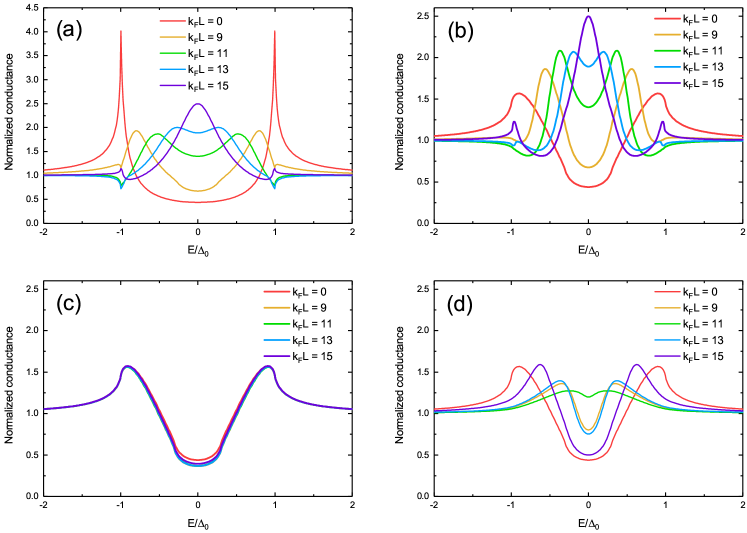
Figure 4: The dimensionless tunneling conductance using pair potentials (a) SW, (b) CPW, $\theta_{M}=0$, (c) HPW, $\theta_{M}=0$ which is identical to CPW, $\theta_{M}=\pi/2$ and (d) HPW, $\theta_{M}=\pi/2$. Without ferromagnet ($k_{F}L=0$) and for varying thicknesses $k_{F}L$ of the ferromagnet. $Z_{1}=0.8$, $X=0.6$.

In the present case, the experimentally observed zero-bias conductance peak (ZBCP)Laube et al. (2000); Mao et al. (2001) does not appear. The Andreev bound states in CPW and HPW superconductors are located in the $b$-$c$ and $c$-$a$ planes. The junction under consideration is, however, along the $c$-axis, implying that these Andreev bound states cannot contribute to the differential conductance.Not

Comparing the red line in Fig. 2(b) to the blue line in Fig. 2(c), we find that the conductance spectra of CPW with $\theta_{M}=\pi/2$ and HPW with $\theta_{M}=0$ are identical. In both cases, the $d$-vector is perpendicular to the magnetization ($\vec{d}\ \bot\ \boldsymbol{M}$), i.e., the total spin of the Cooper pairs is parallel to the magnetization.

By analytically rotating the spin quantization axis, we reduce the matrix form of the pair potential matrix in the proper spin axis in which the $z$-direction is parallel to the magnetization. By doing this, we demonstrate that the pair potentials in the CPW, $\theta_{M}=\pi/2$ and HPW, $\theta_{M}=0$ cases are qualitatively the same, except for the spin-dependent chirality. A full derivation is given in Appendix C; the matrix structures of the pair potential are summarized in table 1. Hence, as far as there is no perturbation which mixes the spins or depends on the chirality (e.g., spin-active interface, spin-orbit coupling, or perturbation which breaks translational symmetry in $x$ and/or $y$ direction such as walls and impurities), it is impossible to distinguish between these two cases.

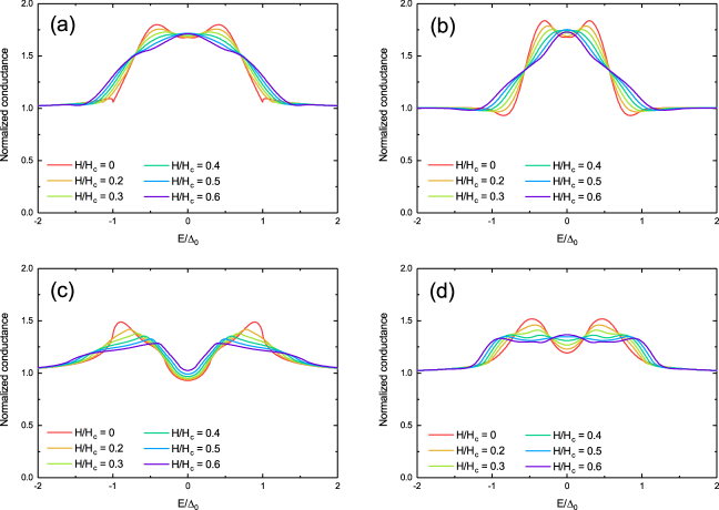
Figure 5: Effects of an external magnetic field on the dimensionless tunneling conductance in the absence of the barrier potential. The pair potential is assumed to be (a) SW, (b) CPW, $\theta_{M}=0$, (c) HPW, $\theta_{M}=0$, and (d) HPW, $\theta_{M}=\pi/2$. The results for the CPW with $\theta_{M}=\pi/2$ are identical to the results in the panel (c). The parameters are set to $Z_{1}=0$, $X=0.6$, and $k_{F}L=11$.

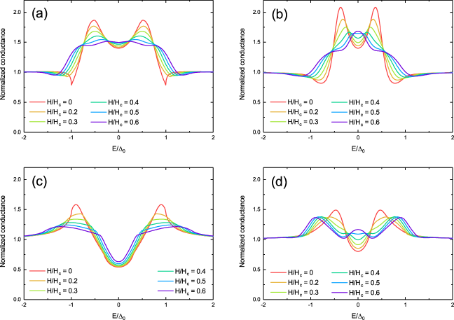
Figure 6: Effects of an external magnetic field on the dimensionless tunneling conductance in the presence of the barrier potential $Z_{1}=0.8$ in the same manner as in Fig. 5.

III.2 Amplitude of the magnetization

The effects of the amplitude of the magnetization are shown in Fig. 3, where the pair potential and the direction of the magnetization are set to (a) SW with $\theta_{M}=0$, (b) CPW with $\theta_{M}=0$, (c) CPW with $\theta_{M}=\pi/2$, and (d) HPW with $\theta_{M}=\pi/2$. We note that the result for the CPW with $\theta_{M}=\pi/2$ and that the HPW with $\theta_{M}=0$ are identical to each other. The barrier strength and the thickness of the ferromagnet are set to $Z_{1}=0.8$ and $k_{F}L=11$, respectively.

In the SW case in the absence of magnetization ($X=0$), we obtain the BTK-like U-shaped spectrumBlonder et al. (1982) as shown in Fig. 3(a). Since the system is regarded as a N/N/S junction when $X=0$, this result is well understood within the BTK theory. When the ferromagnet is fully spin polarised ($X\approx 1$), the conductance becomes zero in the energy range $|E|<\Delta_{0}$. Since there is no propagating channel in the S, a quasi particle with energy $|E|<\Delta_{0}$ must be either normally or Andreev reflected at the F/S interface. In spin-singlet superconductors, Andreev reflection is always accompanied by a spin flip (e.g., an up-spin particle is reflected as a down-spin hole). On the other hand, there is only one band in a fully-polarized ferromagnet, which implies that Andreev reflection is prohibited. As a result, the conductance in the energy range $|E|<\Delta_{0}$ is always zero. For moderate spin polarizations, the conductance spectra have complex structures that are sensitive to the amplitude of $\boldsymbol{M}$.

The conductance spectrum in the CPW, $\theta_{M}=0$ case [Fig. 3(b)] is qualitatively the same as the SW spectrum, because Cooper pairs consist of quasi particles with opposite spin. However, the CPW conductance changes more gradually as a function of magnetization because the amplitude of the pair potential changes depending on $k_{z}$. In the cases where $\vec{d}\ \bot\ \boldsymbol{M}$ [Fig. 3(c)], the conductance spectra do not depend on $\boldsymbol{M}$ qualitatively because the total spin of the Cooper pairs aligns with the magnetization. This implies that the presence of the ferromagnet does not affect the superconductivity and therefore, the conductance spectra are insensitive to the magnetization. Contrary to Figs. 3(a) and 3(b), the conductance in the HPW, $\theta_{M}=\pi/2$ case [Fig. 3(d)] remains finite even if $X\approx 1$. In HPW superconductors, the $d$-vector lies in the $xy$-plain in spin space. Therefore, the $\boldsymbol{k}_{\parallel}$ dependent part of the Andreev reflection is suppressed by the magnetization in the $x$-direction.

III.3 Thickness of the ferromagnet

In Fig. 4, the conductance spectra are plotted for several thicknesses of the ferromagnetic layer $L$. In the SW junction [Fig. 4(a)], the conductance shows the BTK-like U-shaped spectrumBlonder et al. (1982) as seen in Fig. 3(a) with $X=0$. The distance between the two peaks decreases with increasing thickness. Simultaneously, the structures at $E=\Delta_{0}$ change from peaks to dips. When $k_{F}L=15$, the two peaks merge into a ZBCP. We note that this peak is different from the well-known ZBCP in $d$-wave superconductors, which stems from the interference between incident and reflected quasi particles at the interface. On the other hand, the peak at the zero-energy in Fig. 3(a) is formed by an accidental constructive Fabry-Perot interference in the ferromagnet.int Hence, this peak is not robustly resistant to impurities and is therefore not related the topology in the superconductor.

Similar behaviour is seen in the spectrum of the CPW with $\theta_{M}=0$ case [Fig. 4(b)]. In HPW superconductors [Fig. 4(d)], the distance between the two peaks first reduces for $0\leq k_{F}L\leq 11$, whereas it increases for $11\leq k_{F}L\leq 15$. However, the constructive interference as seen in CPW superconductors never occurs at the zero energy. This is a significant difference between CPW and HPW superconductors.

When the $d$-vector is perpendicular to the magnetization (i.e., $\vec{d}\ \bot\ \boldsymbol{M}$), the results are insensitive to the ferromagnet thickness, as shown in Fig. 4(c). This can also be interpreted in terms of the relation between the direction of $\boldsymbol{M}$ and the total spin of Cooper pairs in the superconductor.

III.4 External magnetic field

The magnetic field dependence of the conductance in the absence (presence) of a barrier at the N/F interface is shown in Fig. 5 (Fig. 6), where the other parameters are set to the same values used in Fig. 3. The pair potential is assumed to be (a) SW, (b) CPW with $\theta_{M}=0$, (c) CPW with $\theta_{M}=\pi/2$, and (d) HPW with $\theta_{M}=\pi/2$, where the results for the HPW with $\theta_{M}=0$ are identical to the results in panel (c). We show only the results for an external field $H\leq 0.6H_{c}$, since the effects of the nucleation of vortices are not taken into account.

In general, the Doppler shift causes peaks to split into two smaller peaks, which shift with $k_{\parallel}$, as follows from Eq. (62). Since pairing symmetries have different $k_{\parallel}$-dependencies, the evolution of the peak shape is different in each case. Both SW and CPW with $\theta_{M}=0$ [Figs. 5(a) and 5(b)] show a three dip structure that gradually transitions into a broad ZBCP. For the CPW with $\theta_{M}=\pi/2$ and HPW with $\theta_{M}=0$ cases [Fig. 5(c)], the coherence peaks are smeared out by the magnetic field, although the central dip remains. In the HPW with $\theta_{M}=\pi/2$ case [Fig. 5(d)], the two peaks are split into four smaller peaks [$H/H_{c}=0.4$ in Fig. 5(d)]. The outer peaks shift to away from zero energy, while the inner ones merge and form a small ZBCP.

Including a barrier in the SW, both CPW and HPW, $\theta_{M}=0$ cases [Figs. 6(a)-6(c)] does not change the behaviour qualitatively, but the overall structure is more pronounced. In the HPW, $\theta_{M}=\pi/2$ case [Fig. 6(d)], however, the spectrum changes from a plateau to a three-peak structure. The CPW, $\theta_{M}=0$ and HPW, $\theta_{M}=\pi/2$ cases can be distinguished by looking at the relative peak height of the ZBCP.

IV Summary

We have investigated the conductance of a N/F/S junction with various pair potentials as a function of ferromagnetic properties (thickness, magnetization strength and direction). The SW and CPW, $\theta_{M}=0$ cases are similar, although the latter shows a more rounded conductance due to the angle dependence of the pair potential. We found that the cases where the $d$-vector is perpendicular to the magnetization direction (CPW, $\theta_{M}=\pi/2$ and HPW, $\theta_{M}=0$) are identical. In these cases, the opposite spins parts of the Hamiltonian are decoupled and therefore, they are insensitive to the ferromagnet thickness and magnetization strength. The cases where the $d$-vector is parallel to the magnetization direction are very different due to a more complex structure. The main difference is that CPW, $\theta_{M}=0$ converges to a zero energy peak for $k_{F}L=15$, while HPW, $\theta_{M}=\pi/2$ shows a dip. In the presence of an external magnetic field, the evolution of the conductance spectra depends on the pairing symmetry. In particular, the CPW, $\theta_{M}=0$ case gives an accidental ZBCP. The central dip in the CPW, $\theta_{M}=\pi/2$ and HPW, $\theta_{M}=0$ cases remains. In the HPW, $\theta_{M}=\pi/2$ case, the structure depends on the barrier strength; a plateau or three peaks.

For future research, it would be interesting to take higher applied magnetic fields into account by including Abrikosov vortices. To obtain a more accurate representation of the Sr₂RuO₄, tunneling spectroscopy can be simulated using a multiband model.Yada et al. (2014); Kawai et al. (2017)

Appendix A Doppler shift

In the presence of a magnetic field $\boldsymbol{H}=\boldsymbol{\nabla}\times\boldsymbol{A}$ the canonical momentum operator $\boldsymbol{p}$ is replaced by the kinetic momentum operator $\boldsymbol{\pi}=\boldsymbol{p}-e\boldsymbol{A}(\vec{r})/c$. As a result, the quasi particle kinetic energy $\xi_{k}$ becomes

$$\xi_{k}=\frac{1}{2m}\boldsymbol{\pi}\cdot\boldsymbol{\pi}-\mu=-\frac{\hbar^{2}}{2m}\left(\boldsymbol{\nabla}-i\frac{|e|}{\hbar c}\boldsymbol{A}\right)^{2}-\mu.$$ (56)

where $\mu$ is the chemical potential. In the weak-coupling limit ($\Delta_{0}\ll\mu$), this can be approximated by

$$\xi_{k}\approx-\frac{\hbar^{2}\nabla^{2}}{2m}-i\frac{\hbar|e|}{mc}\boldsymbol{\nabla}\cdot\boldsymbol{A}-\mu.$$ (57)

In our case, an external magnetic field $\boldsymbol{H}$ is applied in the $x$-direction. Hence, the magnetic field and vector potential for $z\geq 0$ are approximatelyFogelström et al. (1997)

$$\boldsymbol{H}(z)=He^{-z/\lambda_{L}}\boldsymbol{e}_{x},$$ (58)

$$\boldsymbol{A}(z)=-H\lambda_{L}e^{-z/\lambda_{L}}\boldsymbol{e}_{y},$$ (59)

where $\lambda_{L}$ is the London penetration depth. The spatial dependence of $\boldsymbol{A}$ is characterized by $\lambda_{L}$, whereas the Cooper pair wave function is characterized by the coherence length $\xi_{0}$. In the type-II limit ($\lambda_{L}/\xi_{0}\gg 1$), the spatial dependence of $\boldsymbol{A}$ does not change the differential conductance. Therefore we introduce the constant vector potentialTanaka et al. (2002)

$$\boldsymbol{A}(z)\approx-H\lambda_{L}\boldsymbol{e}_{y}.$$ (60)

This linear response is only valid in the absence of vortices, i.e. for small magnetic fields ($H\leq 0.6H_{c}$). Assuming plane waves in the $x$- and $y$-direction, the wave function can be written as $\psi(x,y,z)=\psi(z)e^{ik_{x}x}e^{ik_{y}y}$, such that Eq. (57) becomes

$$\xi_{k}=-\frac{\hbar^{2}}{2m}\frac{\partial^{2}}{\partial z^{2}}+\frac{\hbar^{2}k_{\parallel}^{2}}{2m}-\frac{\hbar|e|}{mc}H\lambda_{L}k_{y}-\mu,$$ (61)

where $k_{\parallel}^{2}=k_{x}^{2}+k_{y}^{2}$. Defining $\mu^{\prime}\equiv\mu-\hbar^{2}k_{\parallel}^{2}/2m$ and substituting $H_{c}=\phi_{0}/\pi\xi_{0}\lambda_{L}$, $\phi_{0}=\pi\hbar c/|e|$, $\xi_{0}=\hbar v_{F}/\Delta_{0}$, $k_{y}=k_{\parallel}\sin\varphi$ and $v_{F}=\hbar k_{F}/m$, Eq. (61) can be written as

$$\xi_{k}=-\frac{\hbar^{2}}{2m}\frac{\partial^{2}}{\partial z^{2}}-\mu^{\prime}-\Delta_{0}\frac{H}{H_{c}}\frac{k_{\parallel}}{k_{F}}\sin\varphi,$$ (62)

where $H_{c}$ is the thermodynamical critical field.

Appendix B Numerical method

Substituting wave functions Eqs. (29) and (34) into boundary condition Eq. (49) gives

$$\vec{i}+\vec{r}=\check{A}\left(\vec{f}_{p}+\vec{f}_{n}\right).$$ (63)

We do the same with boundary condition Eq. (50) and divide by $ik_{0}$ for normalization, where we define $k_{0}$ as the momentum in the normal metal, i.e. $k_{0}=\sqrt{2m_{N}\mu}/\hbar$. The second boundary condition becomes

$$\left(\frac{k_{N}}{k_{0}}\check{\tau}_{0}-2i\check{Z}_{1}\right)\vec{i}-\left(\frac{k_{N}}{k_{0}}\check{\tau}_{z}+2i\check{Z}_{1}\right)\vec{r}=\check{A}\check{Q}\left(\vec{f}_{p}-\vec{f}_{n}\right)$$ (64)

where $\check{Q}=\mathrm{diag}[~{}k_{F}^{+},\,~{}k_{F}^{-},\,~{}k_{F}^{+},\,~{}k_{F}^{-}~{}]/k_{0}$ and $\check{Z}_{1}$ is the dimensionless barrier strength of the first interface, given by

$$\check{Z}_{1}=\frac{m(z)\check{F}_{1}}{\hbar^{2}k_{0}}.$$ (65)

We substitute wave functions Eqs. (34) and (40) into the third boundary condition, Eq. (51), to obtain

$$\check{A}\check{K}_{F}^{L+}\vec{f}_{p}+\check{A}\check{K}^{L-}_{F}\vec{f}_{n}=\check{U}\check{K}_{S}^{L}\vec{t},$$ (66)

where we used $\check{K}_{F}^{L\pm}=\left.\check{K}^{\pm}_{F}\right|_{z=L}$ and $\check{K}_{S}^{L\pm}=\left.\check{K}^{\pm}_{S}\right|_{z=L}$ for abbreviation. Similarly, from Eq. (52), we get

$$\check{A}\check{Q}\left(\check{K}_{F}^{L+}\vec{f}_{p}-\check{K}^{L-}_{F}\vec{f}_{n}\right)-2i\check{Z}_{\mathrm{SO}}\check{A}\left(\check{K}_{F}^{L+}\vec{f}_{p}+\check{K}^{L-}_{F}\vec{f}_{n}\right)$$

$$\hskip 142.26378pt=\frac{k_{S}}{k_{0}}\check{U}\check{\tau}_{z}\check{K}^{L}_{S}\vec{t},$$ (67)

where $\check{Z}_{\mathrm{SO}}$ is the dimensionless spin-orbit coupling strength at the second interface, defined as

$$\check{Z}_{\mathrm{SO}}=\frac{m(z)\check{F}_{\mathrm{SO}}}{\hbar^{2}k_{0}}.$$ (68)

Eqs. (63), (64), (66), (67) form a system of 16 equations with 16 unknowns. Substituting Eqs. (66) and (67) into one another, we can write $\check{M}_{1}\vec{f}_{p}=\check{M}_{2}\vec{f}_{n}$, with

$$\check{M}_{1}=\check{A}\check{Q}\check{K}_{F}^{L+}-2i\check{Z}_{\mathrm{SO}}\check{A}\check{K}_{F}^{L+}-\frac{k_{S}}{k_{0}}\check{U}\check{\tau}_{z}\check{U}^{-1}\check{A}\check{K}_{F}^{L+},$$

$$\check{M}_{2}=\check{A}\check{Q}\check{K}_{F}^{L-}+2i\check{Z}_{\mathrm{SO}}\check{A}\check{K}_{F}^{L-}+\frac{k_{S}}{k_{0}}\check{U}\check{\tau}_{z}\check{U}^{-1}\check{A}\check{K}_{F}^{L-}.$$

Combining this with Eq. (64), we can express $\vec{f}_{p}$ and $\vec{f}_{n}$ in terms of $\vec{i}$ and $\vec{r}$ as

$$\vec{f}_{n} =\check{M}_{3}^{-1}(\vec{i}+\vec{r})$$ (69)

$$\vec{f}_{p} =\check{M}_{1}^{-1}\check{M}_{2}\check{M}_{3}^{-1}(\vec{i}+\vec{r}),$$ (70)

where $\check{M}_{3}=\check{A}\left(\check{M}_{1}^{-1}\check{M}_{2}+\check{\tau}_{0}\right)$. Substituting Eqs. (69) and (70) into Eq. (63), we find that

$$\vec{r}=\check{M}_{4}^{-1}\check{M}_{5}\vec{i}$$ (71)

with

$$\check{M}_{4} =\frac{k_{N}}{k_{0}}\check{\tau}_{z}+2i\check{Z}_{1}-\check{A}\check{Q}\left(\check{M}_{1}^{-1}\check{M}_{2}-\vec{\sigma}_{0}\right)\check{M}_{3}^{-1},$$

$$\check{M}_{5} =\frac{k_{N}}{k_{0}}\check{\tau}_{0}-2i\check{Z}_{1}+\check{A}\check{Q}\left(\check{M}_{1}^{-1}\check{M}_{2}-\vec{\sigma}_{0}\right)\check{M}_{3}^{-1}.$$

Using the $\vec{r}$ coefficients, the conductance can be determined by Eq. (54).

Appendix C Rotation of spin quantisation axis

To discuss the spin of Cooper pairs, it is convenient to rotate the spin quantization axis such that the new $z$-axis is parallel to the magnetization $\boldsymbol{M}$. In our case, $\boldsymbol{M}$ is in the $xz$-plane in spin space. Therefore, the rotation should be around the $y$-axis in spin space, which is carried out by the unitary operator

$$\hat{U}(\theta_{M}) =\exp\left[i({\theta_{M}}/{2})\hat{\sigma}_{y}\right]$$ (72)

$$=\hat{\sigma}_{0}\cos\left({\theta_{M}}/{2}\right)+i\hat{\sigma}_{y}\sin\left({\theta_{M}}/{2}\right),$$ (73)

with which we can rotate spin space by an angle $\theta_{M}$. The unitary matrix in Eq. (73) satisfies $\hat{U}^{*}=\hat{U}$ and therefore, the unitary matrix in Nambu space is given by $\check{U}=\mathrm{diag}[\hat{U},\hat{U}^{*}]=\mathrm{diag}[\hat{U},\hat{U}]$. The BdG equation changes accordingly and becomes

$$\check{H}\Psi={E}\Psi\hskip 11.38109pt\rightarrow\hskip 11.38109pt \check{H}^{\prime}\tilde{\Psi}={E}\tilde{\Psi},$$ (74)

with

$$\tilde{\Psi}=\check{U}{\Psi},\hskip 11.38109pt\check{H}^{\prime}=\check{U}\check{H}\check{U}^{\dagger},$$ (75)

$$\Psi=\Big{[}~{}{\psi}_{\uparrow}~{}~{}{\psi}_{\downarrow}~{}~{}{\psi}_{\uparrow}^{\dagger}~{}~{}{\psi}_{\downarrow}^{\dagger}~{}\Big{]}^{T}.$$ (76)

Figure 7: The dimensionless tunneling conductance for CPW, $\theta_{M}=\pi/2$ and HPW, $\theta_{M}=0$, including spin-orbit coupling $Z_{SO}=1$. $Z_{1}=0.8$, $X=0.6$, $k_{F}L=11$.

Only the magnetization term depends on spin in the single-particle Hamiltonian $\hat{h}(z)$. In the new spin basis, the magnetization term for particles and holes is given by, respectively,

$$\hat{U}\big{(}\boldsymbol{M}\cdot\hat{\boldsymbol{\sigma}}\big{)}\hat{U}^{\dagger}=M\hat{\sigma}_{z},$$ (77)

$$\hat{U}\big{(}-\boldsymbol{M}\cdot\hat{\boldsymbol{\sigma}}^{*}\big{)}\hat{U}^{\dagger}=-M\hat{\sigma}_{z}.$$ (78)

The pair potential in the new spin space is

$$\left[\begin{array}[]{cc}&\underline{\hat{\Delta}}_{\boldsymbol{k}_{\parallel}}\\[5.69054pt] -\underline{\hat{\Delta}}^{*}_{-\boldsymbol{k}_{\parallel}}&\\ \end{array}\right]\hskip 5.69054pt\rightarrow\hskip 5.69054pt\left[\begin{array}[]{cc}&\hat{U}\underline{\hat{\Delta}}_{\boldsymbol{k}_{\parallel}}\hat{U}^{\dagger}\\[5.69054pt] -\left[\hat{U}\underline{\hat{\Delta}}_{-\boldsymbol{k}_{\parallel}}\hat{U}^{\dagger}\right]^{*}&\\ \end{array}\right],$$ (83)

where we used the relation $\hat{U}^{*}=\hat{U}$. The superconducting pair potential $\underline{\hat{\Delta}}_{\boldsymbol{k}_{\parallel}}$ is transformed to

$$\hat{U}\underline{\hat{\Delta}}_{\boldsymbol{k}_{\parallel}}\hat{U}^{\dagger}$$

$$=\left\{\begin{array}[]{ll}\Delta_{0}i\hat{\sigma}_{y}&\text{for SW, }\\[5.69054pt] \Delta_{0}\big{(}\bar{k}_{x}+i\chi\bar{k}_{y}\big{)}\big{[}\cos\theta\hat{\sigma}_{x}+\sin\theta\hat{\sigma}_{z}\big{]}&\text{for CPW, }\\[5.69054pt] \Delta_{0}\big{(}\bar{k}_{x}\hat{\sigma}_{0}+i\bar{k}_{y}[\cos\theta\hat{\sigma}_{z}-\sin\theta\hat{\sigma}_{x}]\big{)}&\text{for HPW. }\\[5.69054pt] \end{array}\right.$$ (87)

If we substitute $\theta_{M}=0,\pi/2$, these expressions reduce to the pair potentials in table 1 in the main text.

We focus on CPW, $\theta_{M}=\pi/2$ and HPW, $\theta_{M}=0$. In both cases, the magnetization $\boldsymbol{M}$ is perpendicular to the $d$-vector. In other words, $\boldsymbol{M}$ and the total spin of Cooper pairs are collinear. Therefore, the magnetization does not destroy the Cooper pairs. The $4\times 4$ Hamiltonian matrix can be reduced to two $2\times 2$ matrices:

$$\mathcal{H} =\frac{1}{2}\,\sum_{\boldsymbol{k}_{\parallel}}\int\tilde{\Psi}^{\dagger}(z)\check{H}_{B}(z)\tilde{\Psi}(z)\,dz,$$

$$=\frac{1}{2}\,\sum_{\boldsymbol{k}_{\parallel}}\int\sum_{\alpha=\pm 1}\tilde{\Psi}^{\dagger}_{\alpha}\left[\begin{array}[]{cccc}\xi+\alpha M&\Delta_{\alpha,k_{\parallel}}\\[5.69054pt] -\Delta_{\alpha,-k_{\parallel}}^{*}&-(\xi+\alpha M)\\[2.84526pt] \end{array}\right]\tilde{\Psi}_{\alpha}\,dz.$$ (90)

We have introduced a new basis which depends on the spin sector $\alpha$: $\tilde{\Psi}_{\alpha}(z)=[\,\tilde{\psi}_{\alpha}(z)\hskip 5.69054pt\tilde{\psi}_{\alpha}^{\dagger}(z)\,].$ Eq. (90) implies that the system can be decomposed into the spin-up ($\alpha=1$) and spin-down ($\alpha=-1$) subsystems, where we have redefined the up and down spins for the new spin quantization axis. The $\alpha$-dependent pair potential is given by

$$\Delta_{\alpha,k_{\parallel}}=\left\{\begin{array}[]{ll}\alpha{\Delta_{0}}e^{i\phi}&\text{for CPW, }\theta_{M}=\pi/2,\\[5.69054pt] {\Delta_{0}}e^{i\alpha\phi}&\text{for HPW, }\theta_{M}=0,\\[5.69054pt] \end{array}\right.$$ (93)

where we fix $\chi=1$. In the CPW, $\theta_{M}=\pi/2$ case, the chiralities for up- and down-spin sectors are the same, while the signs of the $\alpha$-dependent pair potential are opposite. In the HPW, $\theta_{M}=0$ case, the chiralities are opposite, while the signs of the $\alpha$-dependent pair potential are equal. Therefore, as far as there is no perturbation which mixes the spins or depends on the chirality ($e.g.$, spin-active interface, spin-orbit coupling and perturbations which breaks translational symmetry in the $x$ and/or $y$ direction such as walls and impurities), it is impossible to distinguish these two cases.

This is demonstrated in Fig. 7, where we introduced spin-orbit coupling at the F/S interface by setting $Z_{SO}=1$. In the absence spin-orbit coupling, these two graphs overlapped as seen in Figs. 3(c), 4(c), 5(c), and 6(c). However, in Fig. 7, we can see that they are indeed slightly different.

References

• Maeno et al. (1994) Y. Maeno, H. Hashimoto, K. Yoshida, S. Nishizaki, T. Fujita, J. G. Bednorz,  and F. Lichtenberg, Nature 372, 532 (1994).
• Ishida et al. (1998) K. Ishida, H. Mukuda, Y. Kitaoka, K. Asayama, Z. Q. Mao, Y. Mori,  and Y. Maeno, Nature 396, 658 (1998).
• Tou et al. (1998) H. Tou, Y. Kitaoka, K. Ishida, K. Asayama, N. Kimura, Y. Onuki, E. Yamamoto, Y. Haga,  and K. Maezawa, Physical Review Letters 80, 3129 (1998).
• Murakawa et al. (2004) H. Murakawa, K. Ishida, K. Kitagawa, Z. Q. Mao,  and Y. Maeno, Phys. Rev. Lett. 93, 167004 (2004).
• Mackenzie and Maeno (2003) A. P. Mackenzie and Y. Maeno, Rev. Mod. Phys. 75, 657 (2003).
• Maeno et al. (2012) Y. Maeno, S. Kittaka, T. Nomura, S. Yonezawa,  and K. Ishida, Journal of the Physical Society of Japan 81, 011009 (2012).
• Rice and Sigrist (1995) T. M. Rice and M. Sigrist, Journal of Physics: Condensed Matter 7, L643 (1995).
• Miyake and Narikiyo (1999) K. Miyake and O. Narikiyo, Phys. Rev. Lett. 83, 1423 (1999).
• Kuwabara and Ogata (2000) T. Kuwabara and M. Ogata, Phys. Rev. Lett. 85, 4586 (2000).
• Nomura and Yamada (2000) T. Nomura and K. Yamada, Journal of the Physical Society of Japan 69, 3678 (2000).
• Nomura and Yamada (2002a) T. Nomura and K. Yamada, Journal of the Physical Society of Japan 71, 404 (2002a).
• Nomura and Yamada (2002b) T. Nomura and K. Yamada, Journal of the Physical Society of Japan 71, 1993 (2002b).
• Arita et al. (2004) R. Arita, S. Onari, K. Kuroki,  and H. Aoki, Phys. Rev. Lett. 92, 247006 (2004).
• Nomura and Yamada (2005) T. Nomura and K. Yamada, Journal of the Physical Society of Japan 74, 1818 (2005).
• Nomura et al. (2008) T. Nomura, D. S. Hirashima,  and K. Yamada, Journal of the Physical Society of Japan 77, 024701 (2008).
• Yanase and Ogata (2003) Y. Yanase and M. Ogata, Journal of the Physical Society of Japan 72, 673 (2003).
• Raghu et al. (2010) S. Raghu, A. Kapitulnik,  and S. A. Kivelson, Phys. Rev. Lett. 105, 136401 (2010).
• (18) M. Sato and M. Kohmoto, Journal of the Physical Society of Japan 69, 3505.
• Kuroki et al. (2001) K. Kuroki, M. Ogata, R. Arita,  and H. Aoki, Phys. Rev. B 63, 060506 (2001).
• Takimoto (2000) T. Takimoto, Phys. Rev. B 62, R14641 (2000).
• Tsuchiizu et al. (2015) M. Tsuchiizu, Y. Yamakawa, S. Onari, Y. Ohno,  and H. Kontani, Phys. Rev. B 91, 155103 (2015).
• Laube et al. (2000) F. Laube, G. Goll, H. v. Löhneysen, M. Fogelström,  and F. Lichtenberg, Phys. Rev. Lett. 84, 1595 (2000).
• Mao et al. (2001) Z. Q. Mao, K. D. Nelson, R. Jin, Y. Liu,  and Y. Maeno, Phys. Rev. Lett. 87, 037003 (2001).
• Tanaka and Kashiwaya (1995) Y. Tanaka and S. Kashiwaya, Phys. Rev. Lett. 74, 3451 (1995).
• Kashiwaya and Tanaka (2000) S. Kashiwaya and Y. Tanaka, Rep. Prog. Phys. 63, 1641 (2000).
• Yamashiro et al. (1997) M. Yamashiro, Y. Tanaka,  and S. Kashiwaya, Phys. Rev. B 56, 7847 (1997).
• Kashiwaya et al. (2011) S. Kashiwaya, H. Kashiwaya, H. Kambara, T. Furuta, H. Yaguchi, Y. Tanaka,  and Y. Maeno, Phys. Rev. Lett. 107, 077003 (2011).
• Yamashiro et al. (1998) M. Yamashiro, Y. Tanaka, Y. Tanuma,  and S. Kashiwaya, J. Phys. Soc. Jpn. 67, 3224 (1998).
• Honerkamp and Sigrist (1998) C. Honerkamp and M. Sigrist, Journal of Low Temperature Physics 111, 895 (1998).
• Kashiwaya et al. (1995) S. Kashiwaya, Y. Tanaka, M. Koyanagi, H. Takashima,  and K. Kajimura, Phys. Rev. B 51, 1350 (1995).
• Kashiwaya et al. (1998) S. Kashiwaya, Y. Tanaka, N. Terada, M. Koyanagi, S. Ueno, L. Alff, H. Takashima, Y. Tanuma,  and K. Kajimura, J. Phys. Chem. Solid 59, 2034 (1998).
• Covington et al. (1997) M. Covington, M. Aprili, E. Paraoanu, L. H. Greene, F. Xu, J. Zhu,  and C. A. Mirkin, Phys. Rev. Lett. 79, 277 (1997).
• Alff et al. (1997) L. Alff, H. Takashima, S. Kashiwaya, N. Terada, H. Ihara, Y. Tanaka, M. Koyanagi,  and K. Kajimura, Phys. Rev. B 55, R14757 (1997).
• Wei et al. (1998) J. Y. T. Wei, N.-C. Yeh, D. F. Garrigus,  and M. Strasik, Phys. Rev. Lett. 81, 2542 (1998).
• Iguchi et al. (2000) I. Iguchi, W. Wang, M. Yamazaki, Y. Tanaka,  and S. Kashiwaya, Phys. Rev. B 62, R6131 (2000).
• Hu (1994) C. R. Hu, Phys. Rev. Lett. 72, 1526 (1994).
• Sato et al. (2011) M. Sato, Y. Tanaka, K. Yada,  and T. Yokoyama, Phys. Rev. B 83, 224511 (2011).
• Tanaka and Kashiwaya (2004) Y. Tanaka and S. Kashiwaya, Phys. Rev. B 70, 012507 (2004).
• Tanaka et al. (2005a) Y. Tanaka, S. Kashiwaya,  and T. Yokoyama, Phys. Rev. B 71, 094513 (2005a).
• Asano et al. (2006) Y. Asano, Y. Tanaka,  and S. Kashiwaya, Phys. Rev. Lett. 96, 097007 (2006).
• Tanaka et al. (2005b) Y. Tanaka, Y. Asano, A. A. Golubov,  and S. Kashiwaya, Phys. Rev. B 72, 140503 (2005b).
• Asano et al. (2011) Y. Asano, A. A. Golubov, Y. V. Fominov,  and Y. Tanaka, Phys. Rev. Lett. 107, 087001 (2011).
• Qi and Zhang (2011) X.-L. Qi and S.-C. Zhang, Rev. Mod. Phys. 83, 1057 (2011).
• (44) G. M. Luke, Y. Fudamoto, K. M. Kojima, M. I. Larkin, J. Merrin, B. Nachumi, Y. J. Uemura, Y. Maeno, Z. Q. Mao, Y. Mori, H. Nakamura,  and M. Sigrist, Nature 394, 558.
• Xia et al. (2006a) J. Xia, Y. Maeno, P. T. Beyersdorf, M. M. Fejer,  and A. Kapitulnik, Phys. Rev. Lett. 97, 167002 (2006a).
• Matsumoto and Sigrist (1999) M. Matsumoto and M. Sigrist, Journal of the Physical Society of Japan 68, 3120 (1999).
• Xia et al. (2006b) J. Xia, Y. Maeno, P. T. Beyersdorf, M. M. Fejer,  and A. Kapitulnik, Phys. Rev. Lett. 97, 167002 (2006b).
• Kirtley et al. (2007) J. R. Kirtley, C. Kallin, C. W. Hicks, E.-A. Kim, Y. Liu, K. A. Moler, Y. Maeno,  and K. D. Nelson, Phys. Rev. B 76, 014526 (2007).
• Hicks et al. (2010) C. W. Hicks, J. R. Kirtley, T. M. Lippman, N. C. Koshnick, M. E. Huber, Y. Maeno, W. M. Yuhasz, M. B. Maple,  and K. A. Moler, Phys. Rev. B 81, 214501 (2010).
• Huang et al. (2014) W. Huang, E. Taylor,  and C. Kallin, Phys. Rev. B 90, 224519 (2014).
• Lederer et al. (2014) S. Lederer, W. Huang, E. Taylor, S. Raghu,  and C. Kallin, Phys. Rev. B 90, 134521 (2014).
• Ashby and Kallin (2009) P. E. C. Ashby and C. Kallin, Phys. Rev. B 79, 224509 (2009).
• Huang et al. (2015) W. Huang, S. Lederer, E. Taylor,  and C. Kallin, Phys. Rev. B 91, 094507 (2015).
• Bouhon and Sigrist (2014) A. Bouhon and M. Sigrist, Phys. Rev. B 90, 220511 (2014).
• Tada et al. (2009) Y. Tada, N. Kawakami,  and S. Fujimoto, New Journal of Physics 11, 055070 (2009).
• Suzuki and Asano (2016) S.-I. Suzuki and Y. Asano, Phys. Rev. B 94, 155302 (2016).
• Hirai et al. (2001) T. Hirai, N. Yoshida, Y. Tanaka, J. ichiro Inoue,  and S. Kashiwaya, Journal of the Physical Society of Japan 70, 1885 (2001).
• Hirai et al. (2003) T. Hirai, Y. Tanaka, N. Yoshida, Y. Asano, J. Inoue,  and S. Kashiwaya, Phys. Rev. B 67, 174501 (2003).
• Yoshida et al. (1999) N. Yoshida, Y. Tanaka, J. Inoue,  and S. Kashiwaya, Journal of the Physical Society of Japan 68, 1071 (1999).
• Li and Yang (2012) H. Li and X. Yang, Solid State Communications 152, 1655 (2012).
• Cheng and Jin (2013) Q. Cheng and B. Jin, Physica B 426, 40 (2013).
• Anwar et al. (2016) M. S. Anwar, S. R. Lee, R. Ishiguro, Y. Sugimoto, Y. Tano, S. J. Kang, Y. J. Shin, S. Yonezawa, D. Manske, H. Takayanagi, T. W. Noh,  and Y. Maeno, Nature Commun. 7, 13220 (2016).
• Gentile et al. (2013) P. Gentile, M. Cuoco, A. Romano, C. Noce, D. Manske,  and P. M. R. Brydon, Phys. Rev. Lett. 111, 097003 (2013).
• Terrade et al. (2013) D. Terrade, P. Gentile, M. Cuoco,  and D. Manske, Phys. Rev. B 88, 054516 (2013).
• Brydon and Manske (2009) P. M. R. Brydon and D. Manske, Phys. Rev. Lett. 103, 147001 (2009).
• Brydon (2009) P. M. R. Brydon, Phys. Rev. B 80, 224520 (2009).
• Wu and Samokhin (2010) S. Wu and K. V. Samokhin, Phys. Rev. B 81, 214506 (2010).
• Blonder et al. (1982) G. E. Blonder, M. Tinkham,  and T. M. Klapwijk, Phys. Rev. B 25, 4515 (1982).
• (69) We note that Eq. (53) is still valid in the presence of spin-rotation. SOC only influences the transport coefficients and does not affect the validity of Eq. (53).
• Chang et al. (2009) Y. J. Chang, C. H. Kim, S.-H. Phark, Y. S. Kim, J. Yu,  and T. W. Noh, Phys. Rev. Lett. 103, 057201 (2009).
• Wu et al. (2014) C.-T. Wu, O. T. Valls,  and K. Halterman, Phys. Rev. B 90, 054523 (2014).
• (72) The condition under which the ABSs emerge is given by $\Delta(k_{z})\Delta(-k_{z})<0$.Asano et al. (2004) All pair potentials in Eq. (28), however, do not depend on $k_{z}$. Therefore, no ABS appears in a junction along the $c$-axis.
• (73) There are two types of the zero-energy conductance peaks. One is a conductance peak which appears accidentally at zero-energy, the other is a conductance peak which should appear at the zero-energy because of, for example, the Andreev interface/surface bound state originating from the topology of the bulk wave functions. A zero-energy peak is not expected on the surface perpendicular to the $c$ direction of Sr2RuO4. Moreover, if the peak in Fig. 3a is caused by, for example, the Andreev bound states in F, the energy of the conductance peek is not affected by the details of a system such as the thickness. In Fig. 3a, the peeks at $\pm\Delta_{0}$ for $L=0$ move in the $\mp E$ direction with increasing $L$. At $k_{F}L=15$, these two peaks merge. For a longer $L$, the two peaks just pass each other.
• Yada et al. (2014) K. Yada, A. A. Golubov, Y. Tanaka,  and S. Kashiwaya, Journal of the Physical Society of Japan 83, 074706 (2014).
• Kawai et al. (2017) K. Kawai, K. Yada, Y. Tanaka, Y. Asano, A. A. Golubov,  and S. Kashiwaya, Phys. Rev. B 95, 174518 (2017).
• Fogelström et al. (1997) M. Fogelström, D. Rainer,  and J. A. Sauls, Phys. Rev. Lett. 79, 281 (1997).
• Tanaka et al. (2002) Y. Tanaka, Y. Tanuma, K. Kuroki,  and S. Kashiwaya, Journal of the Physical Society of Japan 71, 2102 (2002).
• Asano et al. (2004) Y. Asano, Y. Tanaka,  and S. Kashiwaya, Phys. Rev. B 69, 134501 (2004).