A cosmological pathway to testable leptogenesis

Abstract

Leptogenesis could have occurred at temperatures much lower than generally thought, if the cosmological history of the Universe underwent a period of accelerated expansion, as is predicted for example in a class of scalar-tensor theories of gravitation. We discuss how non-standard cosmologies can open new pathways for low scale leptogenesis. Within these scenarios direct tests of leptogenesis could also provide informations on the very early times Universe evolution, corresponding to temperatures larger than the TeV.

1 Introduction

The cosmological baryon asymmetry is very elegantly explained via the leptogenesis mechanism [1] according to which an initial asymmetry is generated in lepton number and then partly converted in a baryon number asymmetry by $B+L$ violating sphaleron processes [2, 3] which, above the temperature of the electroweak (EW) phase transition, proceed with in-equilibrium rates (for reviews on the leptogenesis mechanism see [4, 5]). A very attractive feature of the standard leptogenesis realization based on the type-I seesaw [6, 7, 8, 9] is that it provides a semi-quantitative relation connecting the out-of-equilibrium condition [10] for the decays of the heavy right handed (RH) neutrinos with the light neutrino mass scale. RH neutrino decays can be sufficiently out of equilibrium if $m_{\nu}\sim 10^{-2\pm 1}\,$eV, which is in beautiful agreement with neutrino oscillation data. On the other hand, type-I seesaw leptogenesis has also an unpleasant facet. A lepton asymmetry is preferably generated in the decay of the lightest RH neutrino $N_{1}$ since they generally occur at temperatures when the dynamics of the heavier $N_{2,3}$ neutrino is no more efficient. However, the CP asymmetry in $N_{1}$ decays is bounded by the following relation [11]:

$$\left|\epsilon_{1}\right|\leq\frac{3}{16\pi}\frac{M_{1}}{v^{2}}\frac{\Delta m^{2}_{\oplus}}{m_{1}+m_{3}}\,,$$ (1.1)

where $M_{1}$ is the $N_{1}$ mass, $v\sim 174\,$GeV is the Standard Model (SM) EW breaking vacuum expectation value (VEV), $\Delta m^{2}_{\oplus}\sim 2.4\times 10^{-3}\,{\rm eV}^{2}$ is the atmospheric neutrino mass square difference, and $m_{1,3}$ are the lightest and heaviest light neutrino masses, which are bounded by cosmological data to lie not much above $\sim 10^{-1}\,$eV. Since a minimum CP asymmetry $\left|\epsilon_{1}\right|\ \hbox to0.0pt{\raise 3.0pt\hbox{$>$}\hss}{\lower 3.0pt\hbox{$\sim$}}\ {\rm few}\times 10^{-7}$ is required to account quantitatively for the observed baryon asymmetry, the $N_{1}$ mass cannot lie much below $10^{9}\,$GeV. The conclusion that the CP asymmetry is too small to explain the baryon asymmetry if the leptogenesis scale is too low, implies that direct tests of the standard type-I seesaw leptogenesis are out of experimental reach. Since the argument does not involve any cosmological input, it holds regardless of the assumed cosmological model.

In more generic realization of leptogenesis eq. (1.1) does not necessarily hold: the simple relation between the CP asymmetries and the light neutrino masses is in fact quite specific of the type-I seesaw and is often lost in other models. The most direct way to relax this bound is to rescale $v$ in eq. (1.1) and this can be realized in model where neutrinos only couple through a neutrinophilic Higgs which obtains a VEV $v_{\nu}\ll v$  [19, 20]. Other examples are the inert scalar doublet model [21] complemented with heavy Majorana neutrinos [22], as well as many other models, see [23, 24, 18, 25, 26, 27, 28] for a sample list. Still, the vast majority of models that attempt to generate the baryon asymmetry from heavy particle decays are subject to an additional constraint which, although less tight than the one implied by eq. (1.1), is much more general. This constraint stems from a general relation between the strength of the washout scatterings which tend to erase any lepton number asymmetry present in the thermal bath, and the CP asymmetries in the decays of the heavy states. To our knowledge, in standard cosmologies only models which invoke a resonant enhancement of the CP asymmetries [29, 30, 31, 27] can evade the corresponding bound and bring leptogenesis from heavy particle decays down to a testable scale [32].

In this paper we point out that this conclusion can be avoided if in the very early stages, the cosmological history of the Universe is described by a scalar-tensor gravity (ST) theory [33, 34, 35] rather than by general relativity (GR). ST theories benefit from an attraction mechanism which, prior to Big Bang Nucleosynthesis (BBN), makes them flow towards standard GR [36], so that discrepancies with direct cosmological observations can be avoided. Such a possibility was already put forth in relation to possible large enhancements of the dark matter (DM) relic density with respect to a standard cosmological evolution [37, 38], as a consequence of a modified expansion rate. Many studies on conformally coupled ST models have been performed in [39, 40, 41, 42, 43, 44, 45, 46, 47, 48, 49, 50]. In [49] it was shown that, in comformally coupled ST theories, BBN constraints can be severe and allow only moderate deviations from the standard GR expansion history at the time of DM decoupling so that, based on the boundary conditions and DM masses used in  [37, 38], the enhancement of the DM relic density cannot exceed a factor of three . However, larger DM masses ($\sim 1$ TeV) were considered in ref. [50] where it was shown that the particles undergo a second annihilation process. In that case the enhancement of the relic density can be quite large compared to the standard cosmological evolution. In ref. [51], generalized ST theories were studied after including also disformal couplings [52] and it was concluded that the relic density can be large even for smaller DM masses, with an increase up to a few orders of magnitude compared to the standard GR case. The larger relic density in both conformal and disformal cases is due to the boosted cosmological expansion rate which characterizes ST theories. The magnitude of the enhancement depends on boundary conditions and it can be a few orders of magnitude larger compared to the standard GR expansion. We will make use of this enhancement in the expansion rate in our study of leptogenesis.

Differently from the case of DM, for which the typical decoupling temperature falls in the few GeV range, the generation of a baryon asymmetry via leptogenesis must occur above the EW scale before the EW sphaleron processes get out of equilibrium. Since a leptogenesis scale up to a couple of TeV might still be within the reach of collider tests, we are interested in modifications of the standard cosmology at temperatures in the range $100\,{\rm GeV}-{\rm few}\,{\rm TeV}$. Indeed, due to the larger scale in the game, we find that in the framework of conformally coupled ST theories the modified expansion does allows to lower the scale for successful leptogenesis down to $M_{1}\ \hbox to0.0pt{\raise 3.0pt\hbox{$<$}\hss}{\lower 3.0pt\hbox{$\sim$}}\ 1\,{\rm TeV}$. Hence, in our analysis we will mainly focus on conformally coupled ST theories since this conclusion holds also for ST theories with disformal couplings.

The paper is organized as follows. In sec. 2, we discuss constraints on the leptogenesis scale, in sec. 3, we discuss cosmological scenarios yielding boosted expansion rates. In sec. 4 we present a simple benchmark model which will be used for the leptogenesis analysis. In sec. 5, we discuss the network of Boltzmann equations (BE) for leptogenesis in the modified cosmology, in sec. 6 we discuss our results, in sec. 7, we discuss the enhancement scales in the extensions of the SM, e.g., Minimal Supersymmetric Standard Model (MSSM) and we conclude in sec. 8.

2 Constraints on the leptogenesis scale

The quantum field theory conditions required in order that loop diagrams can generate a lepton ($L$) number (or any other global quantum number) violating CP asymmetry in the decays of an heavy state $X$ are: (i) complex couplings between $X$ and the particles running in the loop (say $Y$ and $Z$); (ii) a CP even phase from the loop factors, which only arises if the $Y,Z$ propagators inside the loops can go on-shell; (iii) $L$ violation inside the loop. Condition (ii) then implies that $Y$ and $Z$ can also participate as external asymptotic states in scattering processes, and condition (iii) implies that these scatterings are necessarily $L$ violating. This means that decay CP asymmetries unavoidably imply $L$ violating washout scatterings [22, 24]. Since the same couplings enter both in the expression for the CP asymmetries and for the washout scattering rates, it is not surprising that a quantitative relation between CP asymmetries and scattering rates can be worked out. A general expression for this relation has been obtained in [24] and reads:

$$\Gamma(YZ\leftrightarrow\bar{Y}\bar{Z})\approx\frac{64}{\pi}\,T\,\left(\frac{T}{M_{X}}\right)^{n}\,\epsilon_{X}^{2}\,,$$ (2.1)

where $\Gamma$ is the rate of the $\Delta L=2$ washout scatterings, $\epsilon_{X}$ is the CP asymmetry in $X$ decays, and $n=0$ for a scalar $X$ decaying into two scalars $Y,Z$; $n=2$ for a fermion $X$ decaying into a fermion and scalar pair, and $n=4$ for a scalar $X$ decaying into two fermions. Note that eq. (2.1) relates scattering washout rates to CP asymmetries without any reference to the cosmological model. In relation to successful leptogenesis, cosmology enters through the requirement that at the relevant temperature $T\sim M_{X}$ the washout rates do not attain thermal equilibrium:

$$\Gamma(YZ\leftrightarrow\bar{Y}\bar{Z})\ \hbox to0.0pt{\raise 3.0pt\hbox{$<$}\hss}{\lower 3.0pt\hbox{$\sim$}}\ \tilde{H}(T)\big{|}_{T\sim M_{X}}\,,$$ (2.2)

where we parametrize the deviations of the expansion in terms of a temperature dependent function $\xi(T)$ multiplying the canonical GR expansion rate $H(T)=1.66\sqrt{g_{*}}\,T^{2}/M_{P}$ (with $g_{\star}$ the relativistic degrees of freedom and $M_{P}=1.22\times 10^{19}$ GeV), namely $\tilde{H}(T)=\xi(T)H(T)$ (two examples of $\xi(T)$ are given in Figure I) .

In the relevant temperature range $T\sim M_{X}$ the out-of-equilibrium condition eq. (2.2) yields:

$$M_{X}\ \hbox to0.0pt{\raise 3.0pt\hbox{$>$}\hss}{\lower 3.0pt\hbox{$\sim$}}\ 1.2M_{P}\frac{\epsilon^{2}_{X}}{\xi(M_{X})}\,.$$ (2.3)

Assuming as a benchmark value $\epsilon_{X}\ \hbox to0.0pt{\raise 3.0pt\hbox{$>$}\hss}{\lower 3.0pt\hbox{$\sim$}}\ 10^{-7}$ as the lowest possible CP asymmetry able to explain $n_{b}/n_{\gamma}\sim 10^{-10}$, we see that standard cosmology with $\xi(T)=1$ yields the (conservative) limit $M_{X}\ \hbox to0.0pt{\raise 3.0pt\hbox{$>$}\hss}{\lower 3.0pt\hbox{$\sim$}}\ 1.4\cdot 10^{5}\,$GeV, so that in any generic model of leptogenesis from heavy particle decays the relevant scale lies well above experimental reach. As an example, we see from the left plot of Figure I that in modified ST cosmologies the function $\xi(T)$ can remain of order $10^{2}$ in an interval centered at $T\sim$ TeV and spanning about two orders of magnitude in $z={\rm TeV}/T$ . Because of the boosted expansion, in the relevant temperature range, the dynamical processes that govern leptogenesis, in particular, the $\Delta L=2$ washout processes discussed above, can more easily go out of equilibrium, rendering viable scales as low as $M_{X}\lesssim\;$TeV for which direct tests can be foreseen.

3 Cosmological expansion in scalar-tensor theories

In ST theories, the gravitational interaction is mediated by both the metric and a scalar field. The cosmological evolution deviates from the standard expansion of the Universe at early times, but an attractor mechanism  [53, 54] relaxes the theory towards GR prior to the onset of BBN. ST theories are often formulated in one of two frames of reference, namely, the Jordan or Einstein frames. As is shown in [52], the most general transformation, physically consistent, between the two metrics of these frames is given by

$$\tilde{g}_{\mu\nu}=C(\phi)g_{\mu\nu}+D(\phi)\partial_{\mu}\phi\partial_{\nu}\phi,$$ (3.1)

where $\tilde{g}_{\mu\nu}$ is metric in the Jordan frame, $C(\phi)$ is the conformal coupling, $g_{\mu\nu}$ is the metric in the Einstein frame and $D(\phi)$ is the so-called disformal coupling. The conformal coupling characterizes the Brans-Dicke class of ST theories [37, 38, 39, 49, 41] and the disformal coupling arises naturally in D-brane models, as discussed in [55].

The respective advantages of these two frames is that the scalar couplings enter through either the gravitational sector (Jordan frame) or the matter sector (Einstein frame), leaving the other sector unaffected. In the Jordan frame matter fields $\Psi$ are coupled directly to the metric, $\tilde{g}_{\mu\nu}$, which means that the matter sector of the action can be written as $S_{Matter}=S_{Matter}(\tilde{g}_{\mu\nu},\Psi)$. Thus, this frame is more convenient for particle physics considerations because the usual observables, e.g. a mass, have their standard interpretation. However, the scalar field couples to the gravitational sector producing a rather cumbersome gravitational field equations.

On the other hand, in the Einstein frame, the matter piece of the action becomes $S_{Matter}=S_{Matter}(g_{\mu\nu},\phi,\partial_{\mu}\phi,\Psi)$. This implies that physical quantities associated with particles (i.e. mass) measured in this frame have a spacetime dependency. However, the gravitational field equations take their standard form, where the Einstein tensor is proportional to the total energy momentum tensor.

The most common strategy followed in the literature  [49, 37, 50, 51] is to determine the cosmic evolution in the Einstein frame, where the cosmological equations take a more straightforward form, and then transform the results over to the Jordan frame. As was already hinted out before, the effect of modified gravity will enter the computation of particle physics processes through the expansion rate, $\tilde{H}$, in the Jordan frame. Thus, for our leptogenesis analysis, we implement the standard BE by including a modified Hubble parameter $\tilde{H}$. In the following paragraphs we will recall some key definitions and we present the equations for ST theories developed in [50, 51] that allow to evaluate $\tilde{H}$.

The action we consider, written in the Einstein frame, is given by

$$S=\frac{1}{2\kappa^{2}}\!\!\int{\!d^{4}x\sqrt{-g}\,R}-\!\!\int{\!d^{4}x\sqrt{-g}\left[\frac{1}{2}(\partial\phi)^{2}+V(\phi)\right]}$$

$$-\!\!\int{\!d^{4}x\sqrt{-\det\left[C(\phi)g_{\mu\nu}+D(\phi)\partial_{\mu}\phi\partial_{\nu}\phi\right]}\,{\cal L}_{M}(\tilde{g}_{\mu\nu})}\,.$$ (3.2)

where $\kappa^{2}\approx 8\pi G$ (see [50]), $\cal{L}_{M}$ is the matter Lagrangian and $V(\phi)$ is the potential of the scalar field.

After considering an homogeneous and isotropic FRW metric $g_{\mu\nu}$,

$$ds^{2}=-dt^{2}+a(t)^{2}dx_{i}dx^{i}\,,$$ (3.3)

where $a(t)$ is the scale factor, the gravitational field equations and the equation of motion for the scalar field become

$$H_{E}^{2}=\frac{\kappa^{2}}{3}\left[\rho_{\phi}+\rho\right]\,,$$ (3.4)

$$\dot{H}_{E}+H_{E}^{2}=-\frac{\kappa^{2}}{6}\left[\rho_{\phi}+3P_{\phi}+\rho+3P\right]\,,$$ (3.5)

$$\ddot{\phi}+3H_{E}\dot{\phi}+\frac{dV}{d\phi}+Q_{0}=0\,,$$ (3.6)

In the previous equations, dots represent derivatives with respect to the time in the Einstein frame, $H_{E}\equiv\frac{\dot{a}}{a}$ is the expansion rate in the Einstein frame. Note that $H_{E}$ is not the same as the expansion rate in standard cosmology, which we denote by $H$. Additionally, $\rho$ and $P$ are the energy density and pressure of the universe written in the Einstein frame. Moreover, the energy density and pressure of the scalar field are $\rho_{\phi}=\frac{1}{2}\dot{\phi}^{2}+V(\phi)$ and $P_{\phi}=\frac{1}{2}\dot{\phi}^{2}-V(\phi)$.

In (3.6) we introduce $Q_{0}$, which is given by

$$Q_{0}=\rho\left[\frac{D}{C}\,\ddot{\phi}+\frac{D}{C}\,\dot{\phi}\left(\!3H_{E}+\frac{\dot{\rho}}{\rho}\right)\!+\!\left(\!\frac{D_{,\phi}}{2C}-\frac{D}{C}\frac{C_{,\phi}}{C}\!\right)\dot{\phi}^{2}+\frac{C_{,\phi}}{2\,C}(1-3\,\omega)\right],\\$$

where $\omega=P/\rho$ is measured in the Einstein frame. $\omega$ can be related to the equation of state parameter in the Jordan frame ($\tilde{\omega}$) , which is the frame where temperature takes the standard interpretation, through $\omega=(1+DC^{-1}\dot{\phi}^{2})\tilde{\omega}$. To calculate $\tilde{\omega}$ in the very early universe, one has to consider the contribution of each particle in the cosmic fluid to the energy density and pressure of the universe. Throughout most of the early radiation era $\tilde{\omega}=1/3$, but once the temperature of the universe drops below the rest mass of each particle, $\tilde{\omega}$ becomes slightly less than one third.

In order to solve the cosmological equations, it is convenient to replace time derivatives of a generic function $f$ with derivatives with respect to the number of e-folds N ($dN=Hdt$), which will be denoted with a prime $f^{\prime}=df/dN$. We also introduce a dimensionless scalar field $\varphi=\kappa\phi$ for convenience.

After combining (3.4), (3.5) and (3.6) one arrives to the so-called master equation, which describes the evolution of the scalar field during any epoch of the universe (see ref. [50]). During the radiation dominated era, $\rho$ dominates over $V$, so that we can take $V\approx 0$. Moreover, in this work, we will focus on the pure conformal case and set $D=0$. Under those considerations, the master equation becomes

$$\frac{2}{1-\varphi^{\prime 2}/6}\,\varphi^{\prime\prime}+\left(1-\omega\right)\varphi^{\prime}+2(1-3\,\omega)\,\alpha(\varphi)=0\,,$$ (3.7)

where $\alpha(\varphi)=\frac{d\ln C^{1/2}}{d\varphi}$. We consider the conformal coupling $C(\varphi)=1+0.1\exp[-8\varphi]$, which has been used in previous works [37, 50, 51].

As was stated earlier, we need the expansion rate in the Jordan frame for our leptogenesis calculation. This expansion rate, $\tilde{H}$, can be written as (see  [50])

$$\tilde{H}^{2}=\frac{\kappa^{2}}{\kappa_{GR}^{2}}\frac{C(1+\alpha(\varphi)\varphi^{\prime})^{2}}{1-\varphi^{\prime 2}/6}\,H^{2}\,,$$ (3.8)

where $H^{2}=\frac{\kappa^{2}_{GR}}{3}\tilde{\rho}$, $\kappa^{2}\simeq\kappa^{2}_{GR}=8\pi G$ and $\tilde{\rho}\sim g(T)T^{4}$ for the radiation dominated era. From this relation the speedup parameter $\xi$ can be defined as

$$\xi\equiv\frac{\tilde{H}}{H}\,.$$ (3.9)

As mentioned above, the evolution of the scalar field is described by (3.7). This equation contains a term that can be interpreted as an effective potential, given by $V_{eff}=\ln C$. During the radiation dominated era, $\omega=1/3$ and the effective potential term disappears. Later on, around the time when the particles of the plasma become non-relativistic, the parameter $\omega$ in the equation of state differs slightly from $1/3$ (see [50]) and the effective potential kicks in. Therefore, the evolution of the scalar field depends on the effective potential, the initial conditions chosen, and the particle content.

In general, both the initial position and velocity of the scalar field can take any positive or negative values. For the conformal factor chosen, we see that if the velocity is positive or zero, the scalar field will roll down the potential and will slow down due to Hubble friction to a final positive value. That is, the conformal factor will evolve rapidly towards 1, and hence the modification to the expansion rate would be negligible (see eq. (3.8)).

A more interesting result arises when considering negative velocities of the scalar field. In this case, the field will start rolling-up the effective potential towards smaller values of the field, eventually turning back down and moving towards its final value. So, if the field starts at a positive value, and given a sufficiently negative initial velocity, it will move towards negative values until its velocity becomes zero and then positive again, as it rolls back down the effective potential. This change in sign for the scalar field will produce a peak in the conformal coupling, which will give rise to a non-trivial modification of the expansion rate $\xi\neq 1$. This particular behavior is shown in Figure I.

The equation of state parameter $\omega$ plays an important role in locating the temperature at which the speedup factor drops back to 1. Slight variations from the radiation dominated value $\omega=1/3$ appear when particles become non-relativistic. So, to calculate $\omega$, one has to take into account all the SM particles and, depending on the specific SM extensions one is dealing with, one would add right-handed neutrinos, supersymmetric partners or other type of heavy species.

In choosing the boundary conditions to solve eq. (3.7), care must be taken to respect the constraints imposed by the post-Newtonian parameters [56, 57, 58, 59, 60] and, most importantly, one has to ensure that by the time of the onset of BBN $\xi\approx 1$.

Another interesting scenario yielding modified Hubble parameters is the pure disformal scenario, which is defined by a conformal coupling equal to one, and a disformal coupling different from zero in eq. (3.1). This scenario is studied extensively in [51] where the authors present the mathematical formalism, solve the necessary equations for the evolution of the scalar field, and find the modifications to the expansion rate for the particular case $D=1/M_{D}^{4}$, where $M_{D}$ is a mass scale motivated by String Theory, and depends on the string coupling and string scale.

In Figure I we also present the speedup factor $\xi$ in a pure disformal case (thin red lines). In this scenario, $M_{D}$ plays the most important role in the location and shape of $\xi$. The maximum $\xi$ happens close to a temperature equal to $M_{D}$. It is interesting to notice that by rescaling $M_{D}$, $\xi$ moves to a higher (or lower) temperature without changing shape.

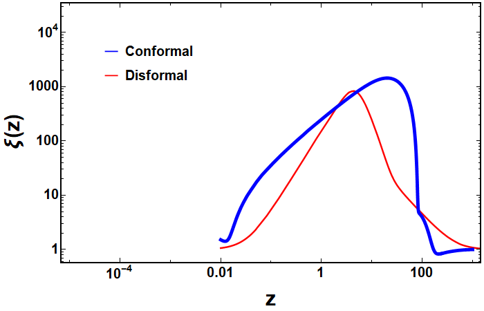
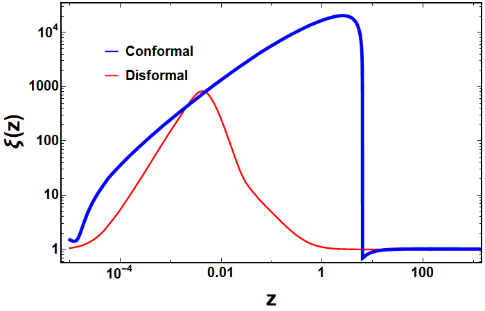
Figure I: Two examples for the speedup factor $\xi(z)$ for conformal (thick blue lines) and disformal (thin red lines) scenarios, as a function of $z=1\,\rm{TeV}/T$ with $T$ the temperature. Left plot: $\xi(z)$ in a conformal scenario with initial conditions $(\varphi_{i},\varphi^{\prime}_{i})=(0.8,-1.83)$ and initial temperature $100\,$TeV, and in a disformal scenario with $(\varphi_{i},\varphi^{\prime}_{i})=(0.2,-2\times 10^{-6})$ and a mass scale $M_{D}=2.5\,$TeV. Right plot: $\xi(z)$ in a conformal and disformal scenario with initial conditions as before, but initial temperature $T=10^{5}\,$TeV, and $M_{D}=2500\,$TeV for the disformal case.

Due to the fact that, as in GR, also in ST cosmologies the total entropy is conserved, adapting the BE for leptogenesis to ST cosmologies is rather straightforward. Considering just the BE for the evolution of the RH neutrinos density $n_{N}$ including only decays and inverse decays will suffice to illustrate this. Denoting with $a$ the scale factor, the BE reads:

$$a^{-3}\frac{d(n_{N}a^{3})}{dt}=\langle\Gamma_{N}\rangle(n_{N}^{0}-n_{N})\,,$$ (3.10)

where $\langle\Gamma_{N}\rangle$ is the thermal averaged decay rate and $n_{N}^{\rm eq}$ the equilibrium density. As usual we use the fiducial variable $z=M_{N}/T$ with $T$ the temperature, and write the time derivative as:

$$\frac{d}{dt}=z\left(\frac{1}{z}\frac{dz}{dt}\right)\frac{d}{dz}=z\left(\frac{1}{a}\frac{da}{dt}\right)\frac{d}{dz}=z\tilde{H}\frac{d}{dz}\,.$$ (3.11)

The second step relies on entropy conservation $d(sa^{3})/dt=0$ with $s\propto T^{3}$ the entropy density which implies the usual temperature-scale factor relation $T\propto 1/a$, while $\tilde{H}$ is the physical Hubble parameter defined as the rate of change of the physical length scale. The rest is standard: denoting by $\gamma_{N}=n_{N}^{\rm eq}\langle\Gamma_{N}\rangle$ the density of the reaction, and normalizing the particle number densities to the entropy density as $Y_{N}=n_{N}/s$ we have:

$$\frac{dY_{N}}{dz}=\frac{1}{sz\tilde{H}}\left(1-\frac{Y_{N}}{Y_{N}^{\rm eq}}\right)\gamma_{N}=\frac{1}{szH}\left(1-\frac{Y_{N}}{Y_{N}^{\rm eq}}\right)\frac{\gamma_{N}}{\xi(z)}\,.$$ (3.12)

In the second equation we have rewritten $\tilde{H}=H\,\xi(z)$ with $H=H_{GR}$ and $\xi(z)>1$ the $T$-dependent speedup factor, to put in evidence how in the BE its effect is equivalent to “slowing down” the decay and inverse decay reactions, favoring the enforcement of the out-of-equilibrium condition.

In the next section, we will show how a simple (non-resonant) leptogenesis model, when embedded in a non-standard cosmology characterized by a boosted expansion rate, allows to get around the constraint eq. (2.3). It is interesting to remark that if a particle physics model can be experimentally established as responsible for the cosmological baryon asymmetry via (non-resonant) baryogenesis via decays of TeV scale particles, this would constitute a direct evidence of non-standard cosmology in a temperature range unreachable by all other cosmological probes (DM freeze-out, EW phase transition, etc.).

4 A simple test model

Besides the generic constraint in eq. (2.3), the type-I (non-resonant) leptogenesis is subject to eq. (1.1) from neutrino mass. In order to get around the latter, a simple way is to assume that the VEV responsible for the neutrino masses is much smaller than the full EW breaking VEV: $v_{\nu}\ll v\sim 174\,$GeV. By requiring a sufficient CP asymmetry $\epsilon_{1}\gtrsim 10^{-7}$, the scale $M_{1}\sim 1\,$TeV can be reached for $v_{\nu}\ \hbox to0.0pt{\raise 3.0pt\hbox{$<$}\hss}{\lower 3.0pt\hbox{$\sim$}}\ 0.2\,$GeV. Of course one has to introduce an ad hoc Higgs field with $\langle H_{\nu}\rangle=v_{\nu}$ coupled to RH neutrinos $N_{j}$ as $\lambda_{j\alpha}\bar{N}_{j}L_{\alpha}H_{\nu}$, and forbid the couplings with the standard Higgs $H$ via some $\mathbb{Z}_{2}$ or $U(1)$ symmetry (a $U(1)$ softly broken might be preferrable to avoid domain wall problems with a spontaneously broken $\mathbb{Z}_{2}$). Such model exists, see for example [19], or [20] for various different possibilities (in the last paper, Model Type I with $m^{2}_{12}>0$ and $\lambda_{5}=0$ is probably the best option). Although the ‘neutrinophilic’ VEV model (we will denote it as $v_{\nu}$-model) might not represent the most elegant possibility, its structure remains very similar to the standard type-I see-saw model, with the advantage that it minimizes the differences with respect to the standard leptogenesis case, rendering it suitable as test model to illustrate the effects of non-standard cosmologies. The usual seesaw formula still holds:

$$m_{\nu}\simeq\lambda^{T}\frac{v^{2}_{\nu}}{M}\lambda,$$ (4.1)

and so does the Casas Ibarra parametrization of the Yukawa couplings:

$$\lambda_{j\alpha}=\frac{1}{v_{\nu}}\sqrt{M_{j}}R_{j\beta}\sqrt{m_{\beta}}(U^{\dagger})_{\beta\alpha}\,,$$ (4.2)

with $M_{j}$ and $m_{\beta}$ the heavy and light neutrino mass eigenvalues, $U$ the neutrino mixing matrix, and $R$ a generic complex orthogonal matrix ($RR^{T}=I$).

Let us consider eq. (4.1). In the usual seesaw with the SM VEV $v\sim 174\,$GeV, to allow for a low value of $M$ while still ensuring $m_{\nu}\ \hbox to0.0pt{\raise 3.0pt\hbox{$<$}\hss}{\lower 3.0pt\hbox{$\sim$}}\ 0.1\,$eV, one has to take tiny Yukawa couplings $\lambda$, which in turn imply tiny CP asymmetries. In the $v_{\nu}$-model instead, the couplings $\lambda$ can be large since it is $v_{\nu}$ that is small, and thus the CP asymmetries can be also large. However, if the scale $M_{1}$ is low, leptogenesis will occur when the Universe expansion is slower, and then the $\Delta L=2$ washouts $LH\leftrightarrow\bar{L}\bar{H}$ or $LL\leftrightarrow\bar{H}\bar{H}$ that are mediated by the same Yukawa couplings can attain thermal equilibrium, realizing the situation in which leptogenesis cannot be successful because of the constraint discussed in sec. 2.

In order to illustrate these constraints in the GR, we show in Figure II the bounds on the lightest RH neutrino mass $M_{1}$ from leptogenesis in the $v_{\nu}$-model as a function of washout parameter defined as

$$K_{1}=\left.\frac{\Gamma_{N1}}{H}\right|_{T=M_{1}}$$ (4.3)

where $\Gamma_{N_{1}}=\frac{(\lambda\lambda^{\dagger})_{11}M_{1}}{8\pi}$ is the total decay width of $N_{1}$. Outside these regions, one cannot generate sufficient baryon asymmetry. Notice that for $K_{1}=1$, the effective neutrino mass is

$${m_{\rm eff}}\equiv\frac{(\lambda\lambda^{\dagger})_{11}v_{\nu}^{2}}{M_{1}}=3.6\times 10^{-8}\sqrt{\frac{g_{\star}}{110.75}}\left(\frac{v_{\nu}}{1\,{\rm GeV}}\right)^{2}\,{\rm eV}.$$ (4.4)

This implies that even in the strong washout regime $K_{1}\gg 1$, the lightest light neutrino remains essentially massless i.e. $m_{1}\approx 0$.

In Figure II, the red/thick and blue/thin lines correspond respectively to values of $v_{\nu}=1,2$ GeV. The solid lines are for the case of vanishing initial $N_{1}$ abundance $Y_{N_{1}}(0)=0$ while dotted lines for thermal initial $N_{1}$ abundance $Y_{N_{1}}(0)=Y_{N_{1}}^{\rm eq}(0)$. The horizontal dashed lines refer to the absolute lower bounds obtained for the respective $v_{\nu}$ if leptogenesis proceeds with $Y_{N_{1}}(0)=Y_{N_{1}}^{\rm eq}(0)$ in the absence of washout (or in the weak washout regime $K_{1}\ll 1$). The lower and upper bounds are respectively due to eq. (1.1) and $\Delta L=2$ washout scattering discussed in sec. 2. Notice that one cannot lower the scale of $M_{1}$ indefinitely by lowing $v_{\nu}$, at some point, the washout will be too strong to generate sufficient baryon asymmetry. This is the case for $v_{\nu}=1$ GeV where no solution exists for the case of $Y_{N_{1}}(0)=0$. In this case, one arrives at lower bound on $M_{1}$ of few times $10^{5}$ GeV in agreement with the estimation in sec. 2.

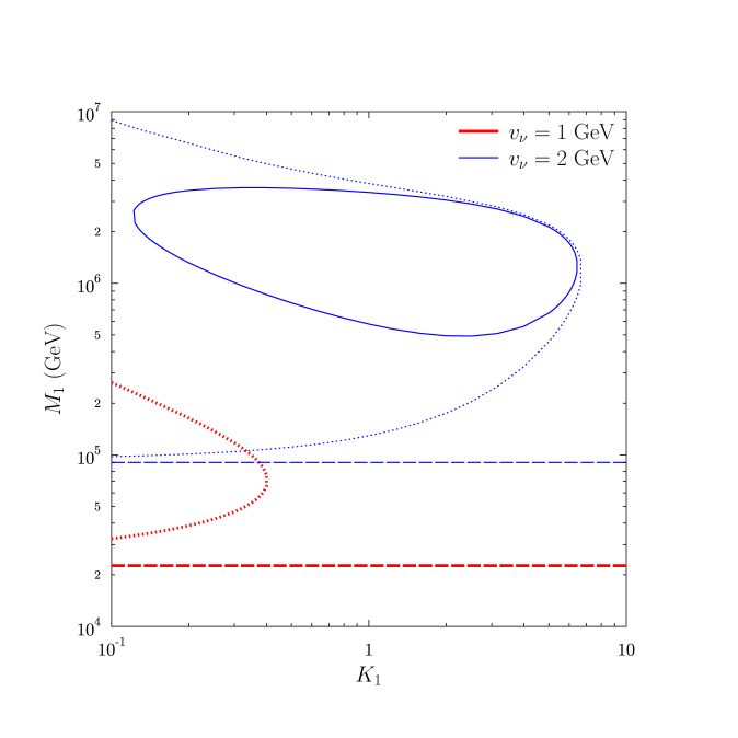
Figure II: The bounds on $M_{1}$ for $v_{\nu}=1,2$ GeV (red/thick, blue/thin lines) as a function of $K_{1}$ defined in eq. (4.3). Outside these closed regimes, one cannot obtain sufficient baryon asymmetry. The solid lines are for zero initial abundance of $N_{1}$ while dotted lines for thermal initial abundance of $N_{1}$. The horizontal dashed lines are the absolute lower bounds obtained for the respective $v_{\nu}$ which correspond to having thermal initial abundance of $N_{1}$ and no washout.

5 Boltzmann equations in the modified cosmology

In the following, we will describe a particle $X$ in term of abundance $Y_{X}\equiv n_{X}/s$ defined as its number density $n_{X}$ normalized over entropic density $s=\frac{2\pi^{2}}{45}g_{\star}T^{3}$. In the following, we will fix $g_{\star}=110.75$ for the SM with an additional (neutrinophilic) Higgs doublet. We start with the following BEs for $Y_{N_{1}}$ and $Y_{\Delta_{\alpha}}$ with $\Delta_{\alpha}\equiv\frac{B}{3}-L_{\alpha}$ as follows

$$s\xi Hz\frac{dY_{N_{1}}}{dz} = -\gamma_{N_{1}}\left(\frac{Y_{N_{1}}}{Y_{N_{1}}^{{\rm eq}}}-1\right),$$ (5.1)

$$s\xi Hz\frac{dY_{\Delta_{\alpha}}}{dz} = -\epsilon_{1\alpha}\gamma_{N_{1}}\left(\frac{Y_{N_{1}}}{Y_{N_{1}}^{{\rm eq}}}-1\right)+\frac{1}{2}P_{1\alpha}\gamma_{N_{1}}\left(\frac{Y_{\Delta\ell_{\alpha}}}{Y_{f}}+\frac{Y_{\Delta H_{\nu}}}{Y_{b}}\right)$$ (5.2)

$$+\gamma_{22}^{\alpha\alpha}\left(\frac{Y_{\Delta\ell_{\alpha}}}{Y_{f}}+\frac{Y_{\Delta H_{\nu}}}{Y_{b}}\right)+\sum_{\beta\neq\alpha}\gamma_{22}^{\alpha\beta}\left(\frac{Y_{\Delta\ell_{\alpha}}}{2Y_{f}}+\frac{Y_{\Delta\ell_{\beta}}}{2Y_{f}}+\frac{Y_{\Delta H_{\nu}}}{Y_{b}}\right),$$

where we have defined $z\equiv\frac{M_{1}}{T}$, $Y_{f}\equiv\frac{15}{8\pi^{2}g_{\star}}$ and $Y_{b}\equiv\frac{15}{4\pi^{2}g_{\star}}$. In the above, $Y_{\Delta\ell_{\alpha}}$ and $Y_{\Delta H_{\nu}}$ refer to abundances per gauge degrees of freedom. Explicitly, the total thermal averaged decay reaction density $\gamma_{N_{1}}$ is given by

$$\gamma_{N_{1}}=\sum_{\alpha}\gamma_{N_{1}\to\ell_{\alpha}H_{\nu}}=n_{N_{1}}^{\rm eq}\Gamma_{N_{1}}\frac{{\cal K}_{1}(z)}{{\cal K}_{2}(z)},$$ (5.3)

where ${\cal K}_{n}(z)$ refers to the modified Bessel function of second type of order $n$ and the branching ratio for $N_{1}$ decay to lepton of flavor $\alpha$ as $P_{1\alpha}\equiv\frac{\gamma_{N_{1}\to\ell_{\alpha}H_{\nu}}}{\gamma_{N_{1}}}$. The $\Delta L=2$ washout mediated by off-shell $N_{i}$ is described by $\gamma_{22}^{\alpha\beta}$. In order to minimize the complication from flavor effects and focus solely on the effect of ST cosmology, we choose the democratic flavor structure as follows

$$\epsilon_{1e} = \epsilon_{1\mu}=\epsilon_{1\tau}\equiv\frac{\epsilon_{1}}{3},$$ (5.4)

$$P_{1e} = P_{1\mu}=P_{1\tau}=\frac{1}{3},$$ (5.5)

$$\gamma_{22}^{\alpha\beta} \equiv \frac{1}{9}\gamma_{22},$$ (5.6)

where $\epsilon_{1}\equiv\sum_{\alpha}\epsilon_{1\alpha}$ and $\gamma_{22}\equiv\sum_{\alpha\beta}\gamma_{22}^{\alpha\beta}$. With the above assumptions, the BE for $Y_{\Delta_{\alpha}}$ becomes

$$s\xi Hz\frac{dY_{\Delta_{\alpha}}}{dz} = -\frac{1}{3}\gamma_{N_{1}}\epsilon_{1}\left(\frac{Y_{N_{1}}}{Y_{N_{1}}^{{\rm eq}}}-1\right)+\frac{1}{6}\gamma_{N_{1}}\left(\frac{Y_{\Delta\ell_{\alpha}}}{Y_{f}}+\frac{Y_{\Delta H_{\nu}}}{Y_{b}}\right)$$ (5.7)

$$+\frac{1}{9}\gamma_{22}\left(\frac{Y_{\Delta\ell_{\alpha}}}{Y_{f}}+\frac{Y_{\Delta H_{\nu}}}{Y_{b}}\right)+\frac{1}{9}\gamma_{22}\left(\frac{Y_{\Delta\ell_{\alpha}}}{Y_{f}}+2\frac{Y_{\Delta H_{\nu}}}{Y_{b}}+\frac{1}{2}\sum_{\beta\neq\alpha}\frac{Y_{\Delta\ell_{\beta}}}{Y_{f}}\right).$$

For $M_{2,3}\gg M_{1}$, the total CP parameter is given by [70]

$$\epsilon_{1} \simeq -\frac{3}{16\pi}\sum_{j>1}\frac{{\rm Im}\left[\left(\lambda\lambda^{\dagger}\right)_{1j}^{2}\right]}{\left(\lambda\lambda^{\dagger}\right)_{11}}\frac{M_{1}}{M_{j}},$$ (5.8)

and using eq. (4.2), one can derive the Davidson-Ibarra bound [11]

$$\left|\epsilon_{1}\right| \leq \frac{3}{16\pi}\frac{M_{1}}{v_{\nu}^{2}}\left(m_{3}-m_{1}\right)\equiv\epsilon_{1}^{{\rm max}},$$ (5.9)

as introduced in eq. (1.1) but with $v\to v_{\nu}$. We further parametrize the off-shell $\Delta L=2$ washout mediated by $N_{i}$ valid for $T<M_{i}$ as follows

$$\gamma_{22} \equiv \frac{n}{\pi^{3}}\frac{{\rm Tr}\left[m_{\nu}m_{\nu}^{\dagger}\right]}{v_{\nu}^{4}}T^{3}=\frac{nM_{1}^{3}}{\pi^{3}z^{3}}\frac{\sum_{i}m_{i}^{2}}{v_{\nu}^{4}},$$ (5.10)

where $n=\frac{2}{\pi^{2}}T^{3}$. As shown in eq. (4.4), the lightest light neutrino mass $m_{1}$ can be neglected and we can rewrite the above in term of eq. (5.9) as follows

$$\gamma_{22} \simeq \frac{256n}{9\pi}\frac{M_{1}}{z^{3}}\epsilon_{1}^{{\rm max},2}.$$ (5.11)

From the above, we see that the $\Delta L=2$ washout is indeed proportional to $\epsilon_{1}^{{\rm max},2}$ as argued in eq. (2.1), so that $M_{1}$ remains bounded from below by the general lower limit given in eq. (2.3). As in the standard type-I seesaw, also in the present case an upper bound on $M_{1}$ exists, which follows from the requirement that $\Delta L=2$ washout scatterings will not become too strong to erase the asymmetry. Eq. (5.10) shows that once the neutrino mass scale $m_{i}$ is fixed, for each value of $v_{\nu}$ there is a limiting upper value of $M_{1}$ for which $\gamma_{22}$ remains sufficiently out of equilibrium. However, while in the standard case this hints to a loose upper limit of order $\sim 10^{14}\,$GeV, due to the large hierarchy $v_{\nu}/v\ \hbox to0.0pt{\raise 3.0pt\hbox{$<$}\hss}{\lower 3.0pt\hbox{$\sim$}}\ 10^{-2}$ and to the quartic dependence on the VEV values, in the neutrinophilic VEV model the corresponding constraint is much stronger.

For the spectator effects [71, 72], we consider the temperature regime $T\lesssim 10^{5}$ GeV where all Yukawa interactions are in chemical equilibrium. We further assume that $H_{\nu}$ does not carry a conserved charge and we have

$$\left(\begin{array}[]{c}Y_{\Delta\ell_{e}}\\ Y_{\Delta\ell_{\mu}}\\ Y_{\Delta\ell_{\tau}}\end{array}\right) = \frac{1}{207}\left(\begin{array}[]{ccc}-64&5&5\\ 5&-64&5\\ 5&5&-64\end{array}\right)\left(\begin{array}[]{c}Y_{\Delta_{e}}\\ Y_{\Delta_{\mu}}\\ Y_{\Delta_{\tau}}\end{array}\right),$$ (5.21)

$$Y_{\Delta H_{\nu}} = -\frac{2}{23}\left(Y_{\Delta_{e}}+Y_{\Delta_{\mu}}+Y_{\Delta_{\tau}}\right).$$ (5.22)

Substituting the result above into eq. (5.7) and summing over $\alpha$ on both sides, the BE becomes

$$s\xi Hz\frac{dY_{\Delta}}{dz} = -\gamma_{N_{1}}\epsilon_{1}\left(\frac{Y_{N_{1}}}{Y_{N_{1}}^{{\rm eq}}}-1\right)+\frac{1}{6}\gamma_{N_{1}}\left(-\frac{6}{23}\frac{Y_{\Delta}}{Y_{f}}-\frac{6}{23}\frac{Y_{\Delta}}{Y_{b}}\right)$$ (5.23)

$$+\frac{1}{9}\gamma_{22}\left(-\frac{6}{23}\frac{Y_{\Delta}}{Y_{f}}-\frac{6}{23}\frac{Y_{\Delta}}{Y_{b}}\right)+\frac{2}{9}\gamma_{22}\left(-\frac{6}{23}\frac{Y_{\Delta}}{Y_{f}}-\frac{6}{23}\frac{Y_{\Delta}}{Y_{b}}\right)$$

$$= -\gamma_{N_{1}}\epsilon_{1}\left(\frac{Y_{N_{1}}}{Y_{N_{1}}^{{\rm eq}}}-1\right)-\frac{3}{23}\left(\gamma_{N_{1}}+2\gamma_{22}\right)\frac{Y_{\Delta}}{Y_{f}},$$

where we have defined $Y_{\Delta}\equiv Y_{\Delta_{e}}+Y_{\Delta_{\mu}}+Y_{\Delta_{\tau}}$. In ref. [73], assuming the SM, it was obtained that the EW sphaleron processes freeze out at $T_{\rm EWSp}=132$ GeV after the EW symmetry breaking at $T_{c}=159$ GeV. Assuming the EW symmetry breaking also happens before $T_{{\rm EWSp}}$ in $v_{\nu}$-model, we have [74, 75]

$$Y_{\Delta B} = \frac{30}{97}Y_{\Delta},$$ (5.24)

excluding the contributions from heavy charged (neutrinophilic) Higgs and top quark.

6 Results

The asymmetry $Y_{\Delta}$ can be parametrized in term of efficiency factor $\eta=\eta(K_{1},v_{\nu},m_{3},M_{1})$ as follows

$$Y_{\Delta} = \epsilon_{1}Y_{N_{1}}^{{\rm eq},0}\eta,$$ (6.1)

where $Y_{N_{1}}^{{\rm eq},0}\equiv Y_{N_{1}}^{{\rm eq}}\left(0\right)=\frac{45}{\pi^{4}g_{\star}}$. The above parametrization is convenient because once we substitute it into eq. (5.23), for temperature-independent $\epsilon_{1}$, the BE becomes independent of $\epsilon_{1}$. The final asymmetry is obtained by evaluating the final efficiency $\eta=\eta(z\to\infty)$. In the case with an initial thermal abundance of $N_{1}$, one saturates to the maximal efficiency $\eta=1$ in limit of weak washout $K_{1}\ll 1$ and small $\Delta L=2$ washout. As we will see in more detail later, as $M_{1}$ gets close to the EW sphaleron freezeout temperature $T_{\rm EWSp}$, one might not be able to saturate the efficiency factor because the baryon asymmetry will be frozen before all $N_{1}$ can decay.

Using eq. (5.9) and eq. (5.24), the maximal asymmetry is given by

$$Y_{\Delta B}^{{\rm max}} = \frac{30}{97}\frac{3}{16\pi}\frac{M_{1}m_{3}}{v_{\nu}^{2}}Y_{N_{1}}^{{\rm eq},0}\eta.$$ (6.2)

Setting $Y_{\Delta B}^{{\rm max}}=Y_{\Delta B}^{{\rm obs}}=8.7\times 10^{-11}$, we can derive both upper and lower bounds on $M_{1}$. Starting from a very small $M_{1}$ while keeping the $\Delta L=2$ washout under control, the CP parameter might be too small and we need to increase $M_{1}$ until $Y_{\Delta B}^{{\rm max}}=Y_{\Delta B}^{{\rm obs}}$, which gives us the lower bound on $M_{1}$. As we continue to increase $M_{1}$, eventually the $\Delta L=2$ washout eq. (5.10) will become too strong until which we are no longer able to obtain sufficient baryon asymmetry and this gives us an upper bound on $M_{1}$. As we explain below eq. (5.11), this upper bound is specific to the model we have chosen due to neutrino mass constraint. In other words, from the following equation

$$M_{1}\eta\left(K_{1},v_{\nu},m_{3},M_{1}\right) = \frac{97}{30}\frac{16\pi}{3}\frac{v_{\nu}^{2}}{m_{3}}\frac{Y_{\Delta B}^{{\rm obs}}}{Y_{N_{1}}^{{\rm eq},0}},$$ (6.3)

for a given $v_{\nu}$ and $m_{3}$, we can have no solution, one solution, or two solutions for $M_{1}$. The two solutions will correspond to upper and lower bounds on $M_{1}$. Notice that as we go to smaller $M_{1}$, the EW sphaleron freezeout temperature becomes relevant and we fix this to be $T_{\rm EWSp}=132$ GeV after which the value of baryon asymmetry will be frozen.

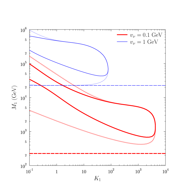
Figure III: The bounds on $M_{1}$ for $v_{\nu}=0.1,1$ GeV (red/thick, blue/thin lines) as a function of $K_{1}$ defined in eq. (4.3). Outside the closed regimes, one cannot obtain sufficient baryon asymmetry. The solid lines are for zero initial abundance of $N_{1}$ while dotted lines for thermal initial abundance. The horizontal dashed lines represent the absolute lower bounds on $M_{1}$ for the respective $v_{\nu}$ obtained with initial thermal abundance of $N_{1}$ and no washout.

It is important to note the temperature where speedup happens is crucial for leptogenesis. As discussed in sec. 3, while the regime of speedup for conformal case depends on initial temperature and $\varphi$ field configurations, the regime of speedup for disformal case depends on a new mass scale $M_{D}$. Besides this point, the qualitative effect of the speedup for both scenarios on leptogenesis remains the same. Hence we will only illustrate the result for speedup factor for conformal case as shown in the left plot of Figure I. In this example where speedup happens in the range $10\,{\rm GeV}<T<10^{5}\,{\rm GeV}$, it will affect leptogenesis with $M_{1}$ which falls in the relevant mass range.

Our main results are presented in Figure III in the $K_{1}-M_{1}$ plane for a fixed $m_{3}=0.05$ eV and $v_{\nu}=0.1,1$ GeV (red/thick, blue/thin lines) where outside these closed regime, one cannot obtain sufficient baryon asymmetry. The solid lines are for $Y_{N_{1}}(0)=0$ while dotted lines for $Y_{N_{1}}(0)=Y_{N_{1}}^{\rm eq}(0)$. The horizontal dashed lines are the absolute lower bounds obtained for the respective $v_{\nu}$ which correspond to having $Y_{N_{1}}(0)=Y_{N_{1}}^{\rm eq}(0)$ and no washout. For $Y_{N_{1}}(0)=0$ and small $K_{1}$, due to the speedup in the Hubble expansion, the inverse decay is not efficient in populating $N_{1}$. Less $N_{1}$ results in less asymmetry being produced and hence $M_{1}$ needs to increase correspondingly to enhance the CP violation. As one goes to larger $K_{1}$, $N_{1}$ is more efficiently populated and one is allowed to have smaller $M_{1}$. Crucially, in all cases, $\Delta L=2$ washout is suppressed sufficiently due to the speedup factor $\xi$ as evidence from the fact that one is able to obtain successful leptogenesis for $M_{1}$ much below $10^{5}$ GeV (cf. Figure II). In fact, a smaller speedup in the early times (see Figure I) allows an efficient washout of an initial ‘wrong’ sign asymmetry (generated during the production of $N_{1}$) by $\Delta L=2$ scattering and one ends up enhancing the final asymmetry. Instead of a curse, $\Delta L=2$ becomes a blessing. Numerically, we found the lowest $M_{1}$ to be around 350 GeV which corresponds to $v_{\nu}\sim 0.03$ GeV and $K_{1}\sim 3000$.

As a final remark, notice that the behaviors of $M_{1}$ lower bounds for $Y_{N_{1}}(0)=Y_{N_{1}}^{\rm eq}(0)$ for small $K_{1}$ are different for the case of $v_{\nu}=0.1,1$ GeV. In the small $K_{1}$ regime, we expect them to approach the absolute lower bounds (the horizontal dashed lines). While this happens for the case of $v_{\nu}=1$ GeV, the lower bound actually moves away from the horizontal line for the case of $v_{\nu}=0.1$ GeV. The reason is that for $M_{1}\sim$ TeV and small $K_{1}$, the decays happen very late close to the EW sphaleron freezeout temperature $T_{\rm EWSp}$. When we reach this temperature, the baryon asymmetry will be frozen before all $N_{1}$ can decay, resulting in smaller final asymmetry.

7 Minimal Supersymmetric Standard Model and right handed neutrinos

In section 3, we mentioned that the scale for the enhanced expansion rate can be moved around as a function of the new scale associated with $D(\varphi)$ term in the disformal case. In the conformal case, an extension of the SM can change the enhancement scale. In this section, we discuss the scale for enhancement in the cases of MSSM and SM with 3 RH neutrinos.

In the left plot of Figure I, we show the speedup factor, in the conformal scenario, for one set of values for $\varphi$ and $\varphi^{\prime}$ at a initial temperature of $100$ TeV considering only the SM particle spectrum. If we add three 10 TeV RH neutrinos, the speedup factor and its slope at around 1 TeV is the same as in the SM case, but $\xi$ drops to 1 slightly earlier.

We now add the RH neutrinos to the spectrum of the SM and MSSM. In Figure IV, we show the enhancements for various values of $\varphi^{\prime}$ and initial temperatures. We add three RH neutrinos at $\sim$ 10 TeV in the particle spectrum along with the SM (solid lines). In the bottom panel of the figure, we show $\omega$ as a function of $z$ (blue solid line) and we find a new small trough at around 10 TeV due to the new RH neutrinos. The other dips in $\omega$ are due to the SM particles. The expansion rate increases when $\varphi^{\prime}$ increases, however if $\varphi^{\prime}$ is too large, the speedup factor does not get reduced to 1 before the BBN. As mentioned before, a sudden drop of the enhancement factor to the standard GR value occurs due to the troughs in $\omega$, which create an attractive effective potential when $\omega\neq 1/3$. For large initial values of $\varphi^{\prime}$, the scalar field overcomes this attractive potential and the enhancement factor never reduces to one.

In Figure IV, left plot, we consider an initial temperature of 100 TeV. The expansion rate can be enhanced by a factor of 100, or more, for temperatures between 100 GeV and 1 TeV. If, however, we increase the initial temperature to $10^{5}$ TeV or higher, the enhancement scale moves to a higher temperature and enhancements bigger than 100 can occur for temperatures between 1 TeV and $10^{4}$ TeV. At higher temperature, the Hubble friction slows down the scalar field faster, and since the attractive effective potential kicks in early, due to the trough in $\omega$ caused by the RH neutrinos (at around 10 TeV), the enhancement factor drops to one at higher temperature.

Using dotted lines in Figure IV, we show the speedup factors due to the MSSM particles, where we keep the SUSY partners of the SM particles at around 1 TeV and, for illustration, three RH neutrinos (and their SUSY partners) at $\sim$ 10 TeV. In the panel below the figure, we show $\omega$ (red dotted line) for MSSM + 3 RH neutrinos and we find a new deep trough in $\omega$ at around 1 TeV due to the SUSY particles (we put all of them together). The other dips are due to the SM particles. Like before, we find that the enhancement and its slope does not change much compared to the SM case but the speedup factor reduces to one for higher temperature.

It is also important to mention, no matter what particle spectrum we consider, that the initial value of the scalar field does not play a relevant roll in the shape and slope of the speedup factor, as long as this value is positive and order one.

We find that an enhancement of the expansion rate with initial temperature at $10^{2-3}$ TeV is most effective in producing a successful leptogenesis, with the enhancement scale around TeV, caused by the SM particle spectrum. Now, the initial temperature is set by the inflation scale. In the case of the MSSM, it is shown that, the thermal leptogenesis constraint from the type I seesaw is $T_{R}>10^{6}$ TeV [76, 77]. This bound conflicts with the cosmological gravitino bound for unstable gravitinos. For a gravitino mass closer to a 100 GeV DM mass, BBN implies stringent upper bound on reheating temperature $\leq O(1)\times 10^{2}$ TeV [78]. Based on our analysis, this low reheating scale is very helpful to have the leptogenesis scale to be around 1 TeV.

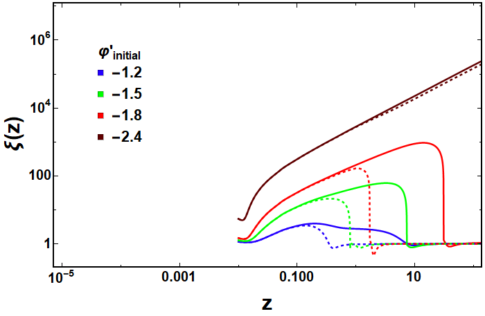
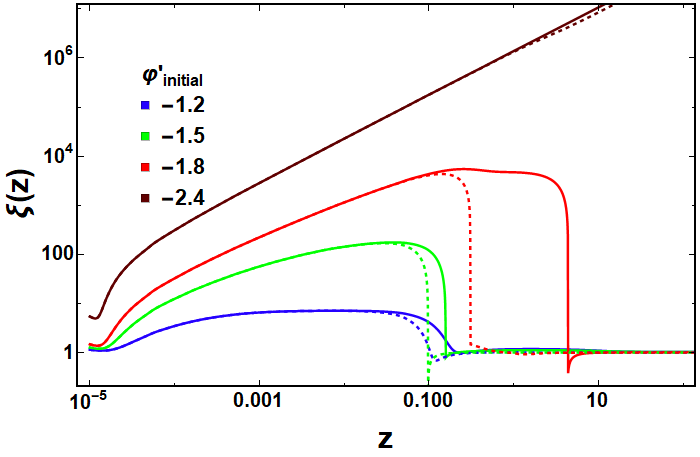
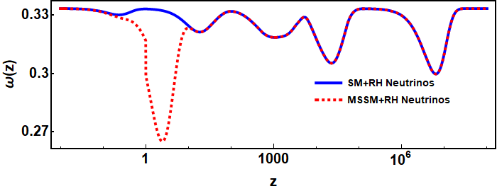
Figure IV: Speedup factor $\xi(z)$ as a function of $z=1\,\rm{TeV}/T$ for SM+3 RH neutrinos (solid lines) and MSSM+3 RH neutrinos (dotted lines) for various values of $\varphi^{\prime}$. The RH neutrinos mass value is $10\,$ TeV, and the initial temperatures are $10^{5}$ GeV (left plot) and $10^{8}$ GeV (right plot). The bottom figure shows the equation of state parameter $\omega$ for the two cases.

8 Concluding remarks

Since it is difficult to probe the universe between inflation and the onset of BBN, the evolution of the universe is mostly unconstrained during this period. Origins of DM, baryon abundances etc. are crucially dependent on the evolution history around that time. During this epoch the expansion rate can be different in ST theories compared to the standard cosmology even though the universe is still radiation dominated. The changes in the expansion rate are caused by conformal and disformal factors in the metric. For an initial temperature set at $\sim$ 100 TeV, the conformal modification of the metric can cause an enhancement in the expansion rate, compared to the standard GR case, by more than two orders of magnitude for temperatures between 100 GeV and a few TeV, due to the SM particles. Although, the size and shape of the enhancements as a function of time are independent of initial $\varphi$ choices, they depend on initial $\varphi^{\prime}$ values. The enhancement scale can move to higher temperatures for extensions of the SM and higher initial temperatures (e.g., $\geq 10^{5}$ TeV). In the case of a disformal scenario, an enhancement can occur at any scale which is determined by the new scale associated with the $\partial_{\mu}\phi\partial^{\mu}\phi$ term in the metric. All these modifications in expansion rates can cause significant changes in the relic dark matter abundance calculations. In this paper, we focused on the effect of an enhancement of the expansion rate on the scale of leptogenesis.

The scale of leptogenesis in the case of a typical type I seesaw model is very high and is out of reach for the ongoing experimental facilities. However, many models with a much lower leptogenesis scale exist where the RH neutrino masses arise due to new physics around multi-TeV scale. In these models, it is found that (if no resonant enhancement of CP asymmetries is assumed), there exists a lower bound on the scale of leptogenesis which is $\sim$ 10 TeV under the assumption of an initial thermal abundance for RH neutrinos along with no washout. The lower bound increases in the case of zero initial abundance. This conclusion changes in ST theories with an enhanced expansion rate which helps the leptogenesis models to be probed in the ongoing experiments.

In the case of an enhanced expansion, the requirement of a larger washout scattering rate demands the scale of leptogenesis to be smaller since the scattering rate is inversely proportional to $M^{n}$ where the exact value of $n$ ($\geq 0$) depends on the details of the initial and final state particle properties. We used a toy model of leptogenesis to manifest the lowering of the leptogenesis scale due to an enhanced expansion rate. In this model the RH neutrinos do not couple to the SM Higgs, instead they couple to a new Higgs. We found that the scale of leptogenesis can be lowered down to $\sim$ TeV for both zero and thermal initial abundances for the RH neutrinos for a wide range of model parameter space which allows these models to be probed at the ongoing experimental facilities. In some parameter space of the model, we showed that an enhancement of the expansion rate can lower the leptogenesis scale down to $\sim 400$ GeV. The existence of an enhanced expansion rate between 100 GeV to a few TeV due to the SM particle spectrum (plus the RH neutrinos) in the case of a conformal modification of the metric is crucial to lower the scale of leptogenesis. If an enhancement happens at a higher scale, the scale of leptogenesis is not lowered and an enhancement at a smaller scale is also not helpful in lowering the leptogenesis scale with the correct amount of asymmetry since the EW sphaleron freezeout occurs at around 130 GeV. All of our findings for this model should apply to any leptogenesis model.

References

- [1] M. Fukugita and T. Yanagida, Baryogenesis Without Grand Unification, Phys. Lett. B174 (1986) 45–47.
- [2] V. A. Kuzmin, V. A. Rubakov, and M. E. Shaposhnikov, On the Anomalous Electroweak Baryon Number Nonconservation in the Early Universe, Phys. Lett. B155 (1985) 36.
- [3] V. A. Rubakov and M. E. Shaposhnikov, Electroweak baryon number non-conservation in the early universe and in high-energy collisions, Usp. Fiz. Nauk 166 (1996) 493–537, [hep-ph/9603208].
- [4] S. Davidson, E. Nardi, and Y. Nir, Leptogenesis, Phys. Rept. 466 (2008) 105–177, [0802.2962].
- [5] C. S. Fong, E. Nardi, and A. Riotto, Leptogenesis in the Universe, Adv. High Energy Phys. 2012 (2012) 158303, [1301.3062].
- [6] P. Minkowski, mu e gamma at a rate of one out of 1-billion muon decays?, Phys. Lett. B67 (1977) 421.
- [7] M. Gell-Mann, P. Ramond, and R. Slansky, Complex spinors and unified theories, . published in Supergravity, P. van Nieuwenhuizen and D.Z. Freedman (eds.), North Holland Publ. Co., 1979.
- [8] T. Yanagida, Horizontal gauge symmetry and masses of neutrinos, . In Proceedings of the Workshop on the Baryon Number of the Universe and Unified Theories, Tsukuba, Japan, 13-14 Feb 1979.
- [9] R. N. Mohapatra and G. Senjanovic, Neutrino Masses and Mixings in Gauge Models with Spontaneous Parity Violation, Phys. Rev. D23 (1981) 165.
- [10] A. D. Sakharov, Violation of CP invariance, C asymmetry, and Baryon Asymmetry of the Universe, Pisma Zh. Eksp. Teor. Fiz. 5 (1967) 32–35.
- [11] S. Davidson and A. Ibarra, A lower bound on the right-handed neutrino mass from leptogenesis, Phys. Lett. B535 (2002) 25, [hep-ph/0202239].
- [12] T. Hambye, M. Raidal, and A. Strumia, Efficiency and maximal CP-asymmetry of scalar triplet leptogenesis, Phys. Lett. B632 (2006) 667–674, [hep-ph/0510008].
- [13] G. Engelhard, Y. Grossman, E. Nardi, and Y. Nir, The Importance of N2 leptogenesis, Phys. Rev. Lett. 99 (2007) 081802, [hep-ph/0612187].
- [14] A. Abada, S. Davidson, F.-X. Josse-Michaux, M. Losada, and A. Riotto, Flavor issues in leptogenesis, JCAP 0604 (2006) 004, [hep-ph/0601083].
- [15] E. Nardi, Y. Nir, E. Roulet, and J. Racker, The Importance of flavor in leptogenesis, JHEP 01 (2006) 164, [hep-ph/0601084].
- [16] A. Abada, S. Davidson, A. Ibarra, F. X. Josse-Michaux, M. Losada, and A. Riotto, Flavour Matters in Leptogenesis, JHEP 09 (2006) 010, [hep-ph/0605281].
- [17] S. Blanchet and P. Di Bari, Flavor effects on leptogenesis predictions, JCAP 0703 (2007) 018, [hep-ph/0607330].
- [18] J. Racker, M. Pena, and N. Rius, Leptogenesis with small violation of B-L, JCAP 1207 (2012) 030, [1205.1948].
- [19] N. Haba and O. Seto, Low scale thermal leptogenesis in neutrinophilic Higgs doublet models, Prog. Theor. Phys. 125 (2011) 1155–1169, [1102.2889].
- [20] J. D. Clarke, R. Foot, and R. R. Volkas, Natural leptogenesis and neutrino masses with two Higgs doublets, Phys. Rev. D92 (2015), no. 3 033006, [1505.05744].
- [21] E. Ma, Verifiable radiative seesaw mechanism of neutrino mass and dark matter, Phys. Rev. D73 (2006) 077301, [hep-ph/0601225].
- [22] J. Racker, Mass bounds for baryogenesis from particle decays and the inert doublet model, JCAP 1403 (2014) 025, [1308.1840].
- [23] D. Aristizabal Sierra, M. Dhen, and T. Hambye, Scalar triplet flavored leptogenesis: a systematic approach, JCAP 1408 (2014) 003, [1401.4347].
- [24] D. Aristizabal Sierra, C. S. Fong, E. Nardi, and E. Peinado, Cloistered Baryogenesis, JCAP 1402 (2014) 013, [1309.4770].
- [25] T. Hambye, Leptogenesis: beyond the minimal type I seesaw scenario, New J. Phys. 14 (2012) 125014, [1212.2888].
- [26] D. Aristizabal Sierra, L. A. Munoz, and E. Nardi, Purely Flavored Leptogenesis, Phys. Rev. D80 (2009) 016007, [0904.3043].
- [27] M. C. Gonzalez-Garcia, J. Racker, and N. Rius, Leptogenesis without violation of B-L, JHEP 11 (2009) 079, [0909.3518].
- [28] D. Aristizabal Sierra, M. Losada, and E. Nardi, Variations on leptogenesis, Phys. Lett. B659 (2008) 328–335, [0705.1489].
- [29] A. Pilaftsis and T. E. Underwood, Resonant leptogenesis, Nucl.Phys. B692 (2004) 303–345, [hep-ph/0309342].
- [30] A. Pilaftsis, Resonant tau leptogenesis with observable lepton number violation, Phys. Rev. Lett. 95 (2005) 081602, [hep-ph/0408103].
- [31] A. Pilaftsis and T. E. J. Underwood, Electroweak-scale resonant leptogenesis, Phys. Rev. D72 (2005) 113001, [hep-ph/0506107].
- [32] E. J. Chun et al., Probing Leptogenesis, 1711.02865.
- [33] P. Jordan, Schwerkraft und Weltall: Grundlagen der theoretische Kosmologie, vol. 107. Vieweg. (Braunschweig: und Sohns), 1955.
- [34] M. Fierz, On the physical interpretation of P.Jordan’s extended theory of gravitation, Helv. Phys. Acta 29 (1956) 128–134.
- [35] C. Brans and R. H. Dicke, Mach’s principle and a relativistic theory of gravitation, Phys. Rev. 124 (1961) 925–935.
- [36] N. Bartolo and M. Pietroni, Scalar tensor gravity and quintessence, Phys. Rev. D61 (2000) 023518, [hep-ph/9908521].
- [37] R. Catena, N. Fornengo, A. Masiero, M. Pietroni, and F. Rosati, Dark matter relic abundance and scalar - tensor dark energy, Phys. Rev. D70 (2004) 063519, [astro-ph/0403614].
- [38] R. Catena, N. Fornengo, M. Pato, L. Pieri, and A. Masiero, Thermal Relics in Modified Cosmologies: Bounds on Evolution Histories of the Early Universe and Cosmological Boosts for PAMELA, Phys. Rev. D81 (2010) 123522, [0912.4421].
- [39] G. B. Gelmini, J.-H. Huh, and T. Rehagen, Asymmetric dark matter annihilation as a test of non-standard cosmologies, JCAP 1308 (2013) 003, [1304.3679].
- [40] T. Rehagen and G. B. Gelmini, Effects of kination and scalar-tensor cosmologies on sterile neutrinos, JCAP 1406 (2014) 044, [1402.0607].
- [41] S.-z. Wang, H. Iminniyaz, and M. Mamat, Asymmetric dark matter and the scalar-tensor model, Int. J. Mod. Phys. A31 (2016), no. 07 1650021, [1503.06519].
- [42] A. Lahanas, N. Mavromatos, and D. V. Nanopoulos, Dilaton and off-shell (non-critical string) effects in Boltzmann equation for species abundances, PMC Phys. A1 (2007) 2, [hep-ph/0608153].
- [43] C. Pallis, Cold Dark Matter in non-Standard Cosmologies, PAMELA, ATIC and Fermi LAT, Nucl. Phys. B831 (2010) 217–247, [0909.3026].
- [44] P. Salati, Quintessence and the relic density of neutralinos, Phys. Lett. B571 (2003) 121–131, [astro-ph/0207396].
- [45] A. Arbey and F. Mahmoudi, SUSY constraints from relic density: High sensitivity to pre-BBN expansion rate, Phys. Lett. B669 (2008) 46–51, [0803.0741].
- [46] H. Iminniyaz and X. Chen, Relic Abundance of Asymmetric Dark Matter in Quintessence, Astropart. Phys. 54 (2014) 125–131, [1308.0353].
- [47] M. T. Meehan and I. B. Whittingham, Asymmetric dark matter in braneworld cosmology, JCAP 1406 (2014) 018, [1403.6934].
- [48] M. T. Meehan and I. B. Whittingham, Dark matter relic density in Gauss-Bonnet braneworld cosmology, JCAP 1412 (2014) 034, [1404.4424].
- [49] M. T. Meehan and I. B. Whittingham, Dark matter relic density in scalar-tensor gravity revisited, JCAP 1512 (2015), no. 12 011, [1508.05174].
- [50] B. Dutta, E. Jimenez, and I. Zavala, Dark Matter Relics and the Expansion Rate in Scalar-Tensor Theories, JCAP 1706 (2017), no. 06 032, [1612.05553].
- [51] B. Dutta, E. Jimenez, and I. Zavala, D-brane Disformal Coupling and Thermal Dark Matter, 1708.07153.
- [52] J. D. Bekenstein, The Relation between physical and gravitational geometry, Phys. Rev. D48 (1993) 3641–3647, [gr-qc/9211017].
- [53] T. Damour and K. Nordtvedt, General relativity as a cosmological attractor of tensor scalar theories, Phys. Rev. Lett. 70 (1993) 2217–2219.
- [54] T. Damour and K. Nordtvedt, Tensor - scalar cosmological models and their relaxation toward general relativity, Phys. Rev. D48 (1993) 3436–3450.
- [55] T. Koivisto, D. Wills, and I. Zavala, Dark D-brane Cosmology, JCAP 1406 (2014) 036, [1312.2597].
- [56] B. Bertotti, L. Iess, and P. Tortora, A test of general relativity using radio links with the Cassini spacecraft, Nature 425 (2003) 374–376.
- [57] S. S. Shapiro, J. L. Davis, D. E. Lebach, and J. S. Gregory, Measurement of the Solar Gravitational Deflection of Radio Waves using Geodetic Very-Long-Baseline Interferometry Data, 1979-1999, Phys. Rev. Lett. 92 (2004) 121101.
- [58] J. G. Williams, X. X. Newhall, and J. O. Dickey, Relativity parameters determined from lunar laser ranging, Phys. Rev. D53 (1996) 6730–6739.
- [59] C. M. Will, The Confrontation between general relativity and experiment, Living Rev. Rel. 4 (2001) 4, [gr-qc/0103036].
- [60] G. Esposito-Farese and D. Polarski, Scalar tensor gravity in an accelerating universe, Phys. Rev. D63 (2001) 063504, [gr-qc/0009034].
- [61] T. Hambye, Y. Lin, A. Notari, M. Papucci, and A. Strumia, Constraints on neutrino masses from leptogenesis models, Nucl. Phys. B695 (2004) 169–191, [hep-ph/0312203].
- [62] M. Raidal, A. Strumia, and K. Turzynski, Low-scale standard supersymmetric leptogenesis, Phys. Lett. B609 (2005) 351–359, [hep-ph/0408015]. [Addendum: Phys. Lett.B632,752(2006)].
- [63] A. Ibarra, E. Molinaro, and S. T. Petcov, TeV Scale See-Saw Mechanisms of Neutrino Mass Generation, the Majorana Nature of the Heavy Singlet Neutrinos and -Decay, JHEP 09 (2010) 108, [1007.2378].
- [64] B. Shuve and I. Yavin, Baryogenesis through Neutrino Oscillations: A Unified Perspective, Phys. Rev. D89 (2014), no. 7 075014, [1401.2459].
- [65] D. Aristizabal Sierra and C. E. Yaguna, On the importance of the 1-loop finite corrections to seesaw neutrino masses, JHEP 08 (2011) 013, [1106.3587].
- [66] E. W. Kolb and S. Wolfram, Baryon Number Generation in the Early Universe, Nucl. Phys. B172 (1980) 224. [Erratum: Nucl. Phys.B195,542(1982)].
- [67] J. N. Fry, K. A. Olive, and M. S. Turner, Evolution of Cosmological Baryon Asymmetries, Phys. Rev. D22 (1980) 2953.
- [68] E. Nardi, J. Racker, and E. Roulet, CP violation in scatterings, three body processes and the Boltzmann equations for leptogenesis, JHEP 09 (2007) 090, [0707.0378].
- [69] C. S. Fong, M. C. Gonzalez-Garcia, and J. Racker, CP Violation from Scatterings with Gauge Bosons in Leptogenesis, Phys. Lett. B697 (2011) 463–470, [1010.2209].
- [70] E. Roulet, L. Covi, and F. Vissani, On the CP asymmetries in Majorana neutrino decays, Phys. Lett. B424 (1998) 101–105, [hep-ph/9712468].
- [71] W. Buchmuller and M. Plumacher, Spectator processes and baryogenesis, Phys. Lett. B511 (2001) 74–76, [hep-ph/0104189].
- [72] E. Nardi, Y. Nir, J. Racker, and E. Roulet, On Higgs and sphaleron effects during the leptogenesis era, JHEP 01 (2006) 068, [hep-ph/0512052].
- [73] M. D’Onofrio, K. Rummukainen, and A. Tranberg, Sphaleron Rate in the Minimal Standard Model, Phys. Rev. Lett. 113 (2014), no. 14 141602, [1404.3565].
- [74] J. A. Harvey and M. S. Turner, Cosmological baryon and lepton number in the presence of electroweak fermion number violation, Phys. Rev. D42 (1990) 3344–3349.
- [75] T. Inui, T. Ichihara, Y. Mimura, and N. Sakai, Cosmological baryon asymmetry in supersymmetric Standard Models and heavy particle effects, Phys. Lett. B325 (1994) 392–400, [hep-ph/9310268].
- [76] W. Buchmuller, P. Di Bari, and M. Plumacher, Leptogenesis for pedestrians, Annals Phys. 315 (2005) 305–351, [hep-ph/0401240].
- [77] G. F. Giudice, A. Notari, M. Raidal, A. Riotto, and A. Strumia, Towards a complete theory of thermal leptogenesis in the SM and MSSM, Nucl. Phys. B685 (2004) 89–149, [hep-ph/0310123].
- [78] M. Kawasaki, K. Kohri, T. Moroi, and A. Yotsuyanagi, Big-Bang Nucleosynthesis and Gravitino, Phys. Rev. D78 (2008) 065011, [0804.3745].