Shape Partitioning via L_p Compressed Modes

Abstract

The eigenfunctions of the Laplace Beltrami operator (Manifold Harmonics) define a function basis that can be used in spectral analysis on manifolds. In [21] the authors recast the problem as an orthogonality constrained optimization problem and pioneer the use of an $L_{1}$ penalty term to obtain sparse (localized) solutions. In this context, the notion corresponding to sparsity is compact support which entails spatially localized solutions. We propose to enforce such a compact support structure by a variational optimization formulation with an $L_{p}$ penalization term, with $0<p<1$. The challenging solution of the orthogonality constrained non-convex minimization problem is obtained by applying splitting strategies and an ADMM-based iterative algorithm. The effectiveness of the novel compact support basis is demonstrated in the solution of the 2-manifold decomposition problem which plays an important role in shape geometry processing where the boundary of a 3D object is well represented by a polygonal mesh. We propose an algorithm for mesh segmentation and patch-based partitioning (where a genus-0 surface patching is required). Experiments on shape partitioning are conducted to validate the performance of the proposed compact support basis.

1 Introduction

Spectral analysis of the Laplace-Beltrami Operator (LBO) on a discrete manifold has found many applications in surface processing, such as for example in shape matching, smoothing, shape recognition, and segmentation [25, 10, 37, 34, 28, 19].

We are in particular interested in two significant surface processing applications of the LBO, namely mesh segmentation (or mesh partitioning) and patch-based partitioning, which are members of a higher level class known as shape partitioning.

Mesh segmentation is fundamental for many computer graphics and animation techniques such as modeling, rigging, shape-retrieval, and deformation. Given an object with arbitrary topology and a discrete manifold representing the object’s boundary, this process consists in the decomposition of an object into salient sub-parts and it relies mostly on surface geometric attributes of the object’s boundary.

Patch-based partitioning has a variety of applications in product design and modeling, reverse engineering, texturing, and 3D printing. By means of this process a discrete manifold is decomposed into smaller patches or sub-manifolds that can be parameterized. Computations can then be performed on simple parameter domains. The patch-based partitioning is often used together with a B-spline surface fitting technology. In general patch-based patching produces discrete sub-manifolds of smaller size with respect to the mesh segmentation.

In recent years, the basis generated by the eigenfunctions of LBO, called Manifold Harmonic Basis (MHB) has been proposed in [32] in analogy to Fourier analysis, and used for example for object segmentation applications [37].

However, in the shape partitioning context, rather than a multiresolution representation of the shape, which is the peculiarity of the MHB on manifolds, the focus is on identifying the observable features of the manifold which represent for example protrusions, ridges, details in general localized in small regions.

Hence, in the partitioning context, a more suitable alternative to the MHB is represented by the Compressed Manifold Basis (CMB), introduced in [20], which is characterized by compact support quasi-eigenfunctions of the LBO obtained by imposing sparsity constraints.

Motivated by the advantages in terms of control on the compact support obtained by using the L₁ norm to force the sparsity of the solution discussed in [21] and [20], we devised to replace the $L_{1}$ norm by a more effective sparsity-inducing L_p norm term, with $0<p\leq 1$, which stronger enforces the locality of the resulting basis functions. The set of functions $\Psi=\left\{\psi_{k}\right\}_{k=1}^{N}$, that we will call $L_{p}$ Compressed Modes ($L_{p}$CMs), is computed by solving the following variational model

$$\min_{\Psi}\sum_{k=1}^{N}\left(\frac{1}{\mu}\|{\psi_{k}}\|_{p}^{p}-\frac{1}{2}<{\psi_{k}},\Delta{\psi_{k}}>\right)\quad s.t.\quad<{\psi_{j}},{\psi_{k}}>=\delta_{jk}$$ (1)

where $\delta_{jk}$ is the Kronecker delta, and $\mu>0$ is a penalty parameter. They form an orthonormal basis for the $L^{2}(\Omega)$ space, where $\Omega$ is the domain in consideration, and they represent a set of quasi-eigenfunctions of the Laplace-Beltrami operator.

The second term in the objective function of (1) is the fidelity term which represents the accuracy of the shape approximation provided by the set of functions $\Psi$, while the first term, so-called penalty term, forces the sparsity in the functions $\Psi$ thus imposing spatially sparse solutions. We remark that at the aim to construct a basis which is sparse but also localized in space it is necessary to further demonstrate that the functions $\Psi$ determined by solving (1) have compact support. This aspect will be proved in this work.

The penalty parameter $\mu$ controls the compromise between the two aspects. It is well known that the sparsity is better induced by the L_p norm for $0<p<1$, rather than the L₁ norm. For $p=1$ model (1) reduces to the proposal in [21], where the sparsity is forced only by acting on the $\mu$ value to increase the contribution of the penalty term, thus decreasing the shape approximation guaranteed by the fidelity term.

The parameter $p$ plays a crucial role since it allows to force the sparsity while maintaining the approximation accuracy without excessively stressing the penalty via the $\mu$ value. The accuracy is fundamental to localize the support of the functions in specific local features of the shape such as protrusions and ridges.

Some evidence of the benefit obtained by the sparsity-inducing proposal, is shown in Fig.LABEL:fig:hand where we try to answer the following question: Can we identify the most salient parts of the manifold hand using only six compressed modes? Fig.LABEL:fig:hand compares the supports of the compressed modes determined as solution of the variational problem (1) with $p=1$ (Fig.LABEL:fig:hand(a)) and $p=0.8$ (Fig.LABEL:fig:hand (b)) where the $\mu$ parameter has been chosen, for each $p$ value, to provide the most natural salient part identification. An automatic strategy for the choice of the optimal $\mu$ parameter will be also discussed in this work. The supports of the six quasi-eigenfunctions are colored in red and we can observe that using $p<1$ strengthens the sparsity, while if $p=1$ no $\mu$ value has allowed to correctly identify all the fingers.

An efficient solution of the orthogonality constrained problem (1) represents a challenging task due to the nonlinear, non-convex orthogonality constraints combined with the non-smooth and non-convex objective function, which may lead to many different local minimizers as solutions. Non-trivial iterative approaches are commonly used to solve this kind of optimization problems. In this paper we propose a variant of the basic Alternating Direction Method of Multipliers (ADMM) approach [6] where the non-convex orthogonality constraints defined for the $L_{p}$ Compressed Modes $\Psi$ in (1) are preserved by means of a SVD matrix factorization, following [14], and a suitable proximal operator is devised to deal with the non-convex penalty.

Although we currently have no proof of convergence for this method, our numerical experiments verify that the method generates a sequence of iterative solutions preserving the orthogonality constraints and decreasing the cost functional in (1). This anyway will motivate future theoretical analysis.

Finally, the proposed ADMM algorithm becomes the kernel of a more sophisticated strategy finalized to the decomposition of a 2-manifold approximated by only a few L_pCMs. The identification and selection of features is a key problem in the context of shape partitioning and the L_pCMs hold the potential for naturally handle this problem thanks to the compact support property that characterizes them.

We devised two methods for generating a suitable L_pCM basis, the first imposes the $\mu$ parameter in (1) while leaving the number of functions free to increase until the shape boundary is completely covered; the second method is based instead on an automatic tuning of the parameter $\mu$ for a fixed number of L_p compressed modes. Once the set of functions $\Psi$ is determined, a region growing process is applied to construct a partitioning of the mesh. A unified algorithm is proposed for both mesh partitioning and a more demanding patch-based partitioning (which guarantee genus-0 patches).

Summarizing, the main contributions are as follows:

• a new variational model for the construction of a compact support basis for the Laplacian operator;

• analysis of the compact support property of the obtained basis functions;

• proposal of an efficient algorithm for the solution of the optimization problem based on ADMM;

• devise of a partitioning algorithm for both shape segmentation and patch-based partitioning based on L_p compressed modes.

The paper is organized as follows. In Section 2 we briefly review the compressed modes and their extension to the 2-manifold context. In Section 3 we introduce the sparsity-inducing variational model to determine the L_pCMs and we provide two important theoretical results. The discretization of the optimization problem on triangulated surfaces is given in Section 4. An efficient ADMM-based iterative algorithm for the solution of the discrete version of (1) is presented in Section 5. Basic notions on the partitioning problem are provided in Section 6 and the algorithmic proposal for both segmentation and patch-based partitioning is described in Section 7. Numerical experiments are presented in Section 8 and conclusions are drawn in Section 9.

1.1 Related work on shape partitioning

Patch-based partitioning and mesh segmentation have been widely studied over recent years, creating a whole categorization of methods based on different methodologies, see [30, 1, 8, 2, 27].

In order to partition a mesh, the spectral analysis methods use the eigenvalues of properly defined matrices, called affinity matrices, based on the connectivity of the mesh. The authors in [18] define an affinity matrix using both geodesic and angular distances. The spectral analysis is performed on the Laplacian matrix weighted by dihedral angle differences in [37], and by mean curvature in [12], and then successfully applied to mesh partitioning. In [7] an affinity matrix is proposed based on the optimal normalized Cheeger cut which encodes both the structural and the geometrical information in order to segment concave regions.

The results of the methods in the class of spectral-based mesh segmentation strongly depend on the affinity matrix considered. In the proposed approach good quality results are obtained simply from the Laplace-Beltrami spectral decomposition, by imposing suitable constraints of orthogonality and sparsity.

In [30], patch-based partitioning is named surface-type segmentation and what is here defined as mesh segmentation is instead referred as part-type segmentation.

An important result on part-type segmentation has been presented in [37], where a convexified version of the variational Mumford-Shah model is presented and extended to 3D meshes. In reverse engineering and Computer Aided Design (CAD) applications, patch-based partitioning is seen as an automatic procedure to create CAD models from measured data, [33]. Patch-based partitioning in [35] is finalized to fitting quadric surfaces to the mesh, while in [17] a smooth stitch of spline patches is built. However, the success of any patch-based method strongly depends on the goodness of the underlying shape partitioning.

We propose a unified framework to perform both mesh segmentation and patch-based partitioning. The proposed method carries out two approaches, one completely unsupervised, namely the number of segments is determined automatically, and the other supervised, by performing a segmentation into a given number of parts. We refer the reader to [31] for unsupervised state-of-the-art methods, and to [5, 13] for supervised competitors.

2 Background on Compressed Modes

In the preliminary work [21] the authors show how to produce a basis of localized functions $\{\psi_{k}\}_{k=1}^{N}$ in ${\mathbb{R}}^{d}$, called Compressed Modes (CMs), by solving the following variational problem

$$\min_{\left\{\psi_{1},\psi_{2},..,\psi_{N}\right\}}\sum_{k=1}^{N}\left(\frac{1}{\mu}\|{\psi_{k}}\|_{1}+\left\langle{\psi_{k}},H{\psi_{k}}\right\rangle\right)\quad s.t.\quad<{\psi_{j}},{\psi_{k}}>=\delta_{jk},$$ (2)

where $H=-\frac{1}{2}\Delta+V(x)$ is the Hamiltonian operator corresponding to potential $V(x)$, the $L_{1}$ norm is defined as $\|f\|_{1}=\int_{\Omega}|f|dx$ and $\left\langle f,g\right\rangle=\int_{\Omega}f^{*}gdx\;\Omega\subset{\mathbb{R}}^{d}$. Here the L₁ norm is a penalty term used to achieve spatial sparsity. The orthonormality constraints in (2), which enforce the orthonormality of the basis functions, lead to a non-convex variational problem, with many local minimizers.

A theoretical analysis of the CMs, provided in [4], allows for finding the minimizer of the variational formulation of the Schrodinger equation, showing the spatial localization property of CMs, and establishing an upper bound on the volume of their support. Consistency results for the CMs were proved in [3].

In [20] the variational problem (2) in ${\mathbb{R}}^{d}$ domains has been extended to deal with Laplace-Beltrami eigenfunctions on 2-manifolds discretized by three-dimensional meshes. These new basis functions, named Compressed Manifold Modes (CMM), form the Compressed Manifold Basis (CMB) and define an alternative to the classical MHB, proposed in [32]. It is well known that the eigenfunctions of the Laplace Beltrami operator, called Manifold Harmonics (MH), define a function basis. In particular, for a smooth manifold $\mathcal{M}$ embedded in ${\mathbb{R}}^{3}$ the Laplace-Beltrami operator induces a set of eigenfunctions $\{\phi_{k}\}$ and associated eigenvalues $\{\lambda_{k}\}$ determined by

$$-\Delta\phi_{k}=\lambda_{k}\phi_{k}\qquad k\in{\mathbb{N}},\;\lambda_{k}\in{\mathbb{R}}.$$ (3)

The self-adjointness of $\Delta$ implies that the eigenvalues are real and that the eigenfunctions are orthogonal with respect to the L₂-inner product: $<f,g>=\int_{\mathcal{M}}f\;g$.

One major drawback of this basis is that, similarly to the Fourier spectrum, the MHs are dense and have global spatial support. This means that the functions do not give intuitive insight on the features of the manifold, thus reducing their use in practical shape processing applications [16]. However, it is well known that using a reduced number of eigenfunctions corresponding to the smallest eigenvalues $\lambda$, the MHs allow to approximate the shape of the manifold in an improved manner as the number of eigenfunctions increases.

3 The sparsity-inducing variational model for L_pCMs

Let $\Omega=B(0,R)\subset{\mathbb{R}}^{d}$ denote the $d$-dimensional ball of radius $R$ centered at the origin. Relation (1) can be rewritten as:

$$\min_{\Psi}\sum_{k=1}^{N}\left(\frac{1}{\mu}\int_{\Omega}{\left|{\psi_{k}}\right|^{p}dx}-\frac{1}{2}\int_{\Omega}{{\psi_{k}}\Delta{\psi_{k}}dx}\right)\quad s.t.\quad\int_{\Omega}{{\psi_{j}}\,{\psi_{k}}\,dx}\,=\,\delta_{jk},$$ (4)

where we denoted the $L_{p}$ norm of a function by $\|f\|_{p}=\left(\int_{\Omega}|f|^{p}dx\right)^{1/p}$.

Before proceeding with the solution of the variational model (4) we demonstrate in the following two important properties of the L_p compressed functions such as local support and completeness, which also hold for the CMs determined by solving (2).

3.1 On the support of the L_pCMs

In this subsection we establish an asymptotic upper bound on the volume of the support of the L_pCMs in terms of the penalty parameter $\mu$ and the sparsity parameter $p$. At this aim, we first reformulate (4) by using integration by parts and imposing zero boundary conditions on $\Omega$. It follows that the first $N$ compressed modes $\left\{\psi_{i}\right\}_{i=1}^{N}$ solve the following constrained optimization problem:

$$\min_{\Psi}\sum_{i=1}^{N}\left(\frac{1}{\mu}\int_{\Omega}{\left|{\psi_{i}}\right|^{p}dx}+\frac{1}{2}\int_{\Omega}{\left|\nabla{\psi_{i}}\right|^{2}dx}\right)\quad s.t.\quad\int_{\Omega}{{\psi_{j}}{\psi_{k}}dx}=\delta_{jk}.$$ (5)

We first introduce the following result on the volume support of the first compressed mode.

Proposition 1.

$\forall x\in\Omega$, any $0<p$ $<$ $1$, and $\mu$ sufficiently small, we have

$$\int_{\Omega}{\left(\frac{1}{\mu}\left|{\psi_{1}}\right|^{p}+\frac{1}{2}\left|\nabla{\psi_{1}}\right|^{2}\right)dx}\leq m(\Omega)^{\frac{1}{p}-1}\mu^{-\frac{4}{4+d}}$$ (6)

where $m(\Omega)$ is the finite measure of the domain $\Omega\subset{\mathbb{R}}^{d}$.

Proof.

From the relation between $L_{p}$ norm and $L_{q}$ norm, with $0<p<q\leq\infty$

$$\|f\|_{p}\leq m(\Omega)^{\frac{1}{p}-\frac{1}{q}}\|f\|_{q},$$ (7)

for $q=1$ and $0<p<1$, it follows that

$$\int_{\Omega}{\left(\frac{1}{\mu}\left|{\psi_{1}}\right|^{p}+\frac{1}{2}\left|\nabla{\psi_{1}}\right|^{2}dx\right)}\leq m(\Omega)^{\frac{1}{p}-1}\cdot\int_{\Omega}{\left(\frac{1}{\mu}\left|{\psi_{1}}\right|+\frac{1}{2}\left|\nabla{\psi_{1}}\right|^{2}\right)dx.}$$ (8)

By using Proposition 3.4 of [4], namely

$$\int_{\Omega}{\left(\frac{1}{\mu}\left|{\psi_{1}}\right|+\frac{1}{2}\left|\nabla{\psi_{1}}\right|^{2}\right)dx}=C_{1}\mu^{-\frac{4}{4+d}},$$

where $C_{1}$ is some fixed constant depending on $d$, we easily obtain the bound in (6). ∎

Theorem 1.

There exist $\mu_{0}$, such that for $\mu<\mu_{0}$ the corresponding L_p compressed modes $\left\{\psi{{}_{i}}\right\}_{i=1}^{N}$ satisfy

$$\left|supp(\psi_{i})\right|\leq C\mu^{-\frac{8}{4+d}+1}m(\Omega)^{\frac{1}{p(1-p)}-2}$$ (9)

where $C$ depends on $N$ and $p$.

The proof is postponed to the appendix.

The result in Theorem 9 is fundamental for the construction of a compact support L_pCM basis and it will represent the key aspect for the shape partitioning method based on the L_pCMs that will be described in Section 7.

An example demonstrating the essence of Theorem 9 is shown in Figure 2. In each row three L_pCM functions are illustrated obtained for a particular $\mu$ value, and fixed $N$ and $p$ values. Since the upper bound given in (9) depends on $\mu,p,N$, for increasing values of $\mu$, as we expected, we notice an enlargement of the compact support of each function.

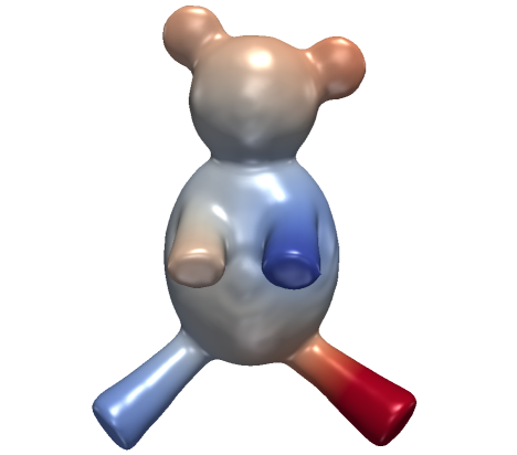
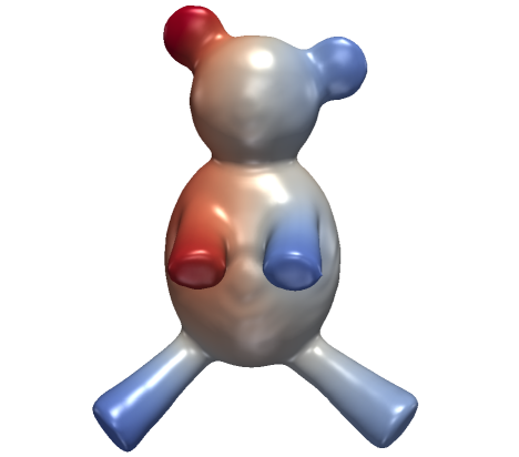
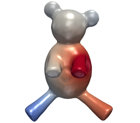
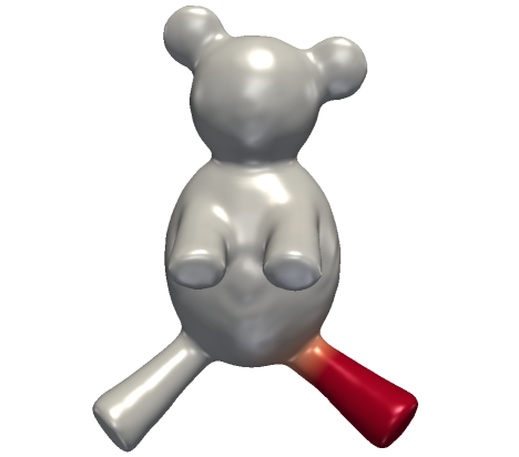
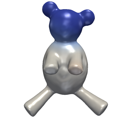
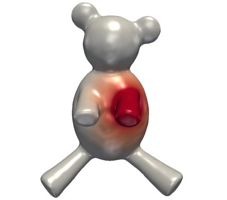
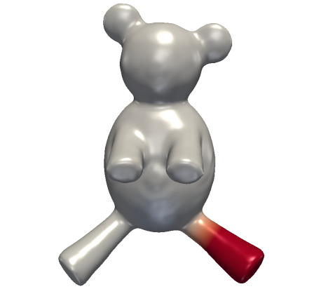
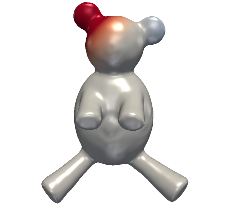
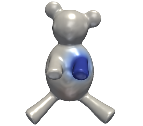
Fig. 2: Three L_pCMs generated for the teddy_2 mesh for three different $\mu$ values, row-wise $\mu=\{250,160,50\}$

3.2 Completeness of the $L_{p}$CMs

We now investigate a completeness result on the $L_{p}$CMs and its effect on shape approximation. In particular, we prove that, for a fixed $\mu$ value in (4), under some unitary transformations, the $L_{p}$CM functions $\left\{\psi_{i}\right\}_{i=1}^{N}$ approximate the eigenfunctions of the Laplacian operator in an improved manner as $N$ increases.

Let $\Phi=\left\{\phi_{i}\right\}_{i=1}^{M}$ be the set of orthonormal eigenfunctions of $-\frac{1}{2}\Delta$ corresponding to the eigenvalues $\left\{\lambda_{i}\right\}_{i=1}^{M}$, defined by (3) where the eigenvalues are arranged in non-decreasing order.

The following result of completeness for the $L_{p}$CMs holds.

Theorem 2.

Given fixed parameters $\mu$ and $p$ in (4), for a fixed integer $M<N$, the first $N$ functions $L_{p}$CMs $\left\{\psi_{i}\right\}_{i=1}^{N}$ up to an unitary transformation, satisfy

$$\lim_{N\rightarrow\infty}\|\phi_{i}-\psi_{i}\|_{2}^{2}=0,\quad i=1,\ldots,M.$$ (10)

Proof.

The proof follows from [36], where the authors demonstrate the result in the case of $L_{1}$-norm, but it still holds if the $L_{1}$ norm term is replaced by any functional bounded by $L_{2}$ norm. In fact, for the relation (7) between $L_{p}$ and $L_{q}$ norms, $0<p<q\leq\infty$, if we set $q=2$, it follows that $L_{p}$-norm, $0<p<2$, is bounded by $L_{2}$-norm. ∎

The completeness result confirms that using the $L_{p}$CM orthogonal basis, analogously to the $\Phi$ basis, we can reconstruct any function defined on the shape, up to an arbitrary degree of precision. However, for a small number $N$ of functions, the approximated reconstructions show significant differences.

By the way of illustration, let us consider the geometric reconstruction of the 2-manifold horse.The shape approximation process, described for MHs in [32], also holds for L_pCMs. The reconstruction obtained by using all the $N$ eigenfunctions of the LBO, where $N=868$, is shown in Fig.3 (top).

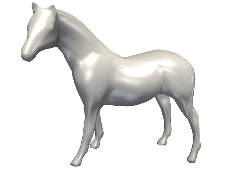
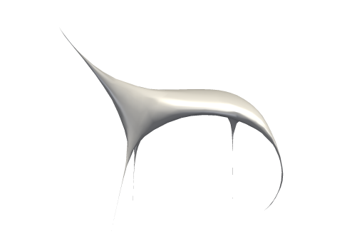
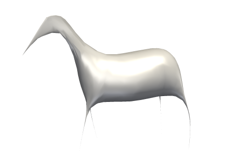
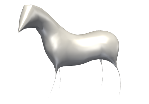
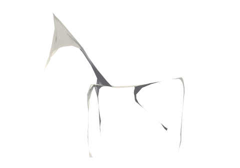
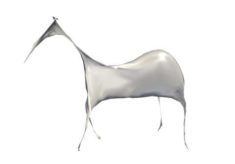
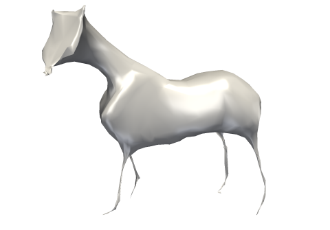
Fig. 3: Reconstruction of the horse shape (top) using MH (middle row) and L_pCM (bottom row) bases for increasing space dimension $N$; from left to right $N=8$, $N=15$, and $N=30$.

In the second and third row of Fig.3 we show, respectively, the shape reconstructions obtained using the basis MHB computed by solving (3), and the proposed L_pCM basis obtained by (4), formulated in the 2-manifold context which will be discussed in the following sections. For a fixed value of the dimension $N$ in the range $N=8,15,30$, the reconstruction obtained by MHB is smoother but less representative of the underlying shape, while the L_pCM approximation looks like a more stylized shape, roughly a skeleton of the shape. Moreover, while the MHB approximations for increasing dimensions tend to refine the basic shape, the L_pCM basis enriches the skeleton shape with smaller features while maintaining the structure of the shape. This can be observed in the horse reconstructions in Fig.3 (bottom) where the horse’s legs and ears are well represented only using the L_pCM bases.

4 Discretization of the variational model

We are interested in the application of model (1) to compute the $L_{p}$ Compressed Modes induced by the LBO on a manifold $\mathcal{M}$. We approximate $\mathcal{M}$ by a triangulated surface mesh $M:=(V,T)$, where $V=\{X_{1},\cdots,X_{n}\}$ is the set of $n$ vertices, $T$ is the connectivity graph, and we denote by $\mathcal{E}\subseteq{V}\times{V}$ the set of edges. Each vertex $X_{i}\in V$ has immediate neighbors $X_{j},j\in N(X_{i}),$ to which it is connected by a single edge $e_{ij}$. We denote by $N_{\triangle}(X_{i})$ the set of triangles with vertex $X_{i}$, and by $|N_{\triangle}(X_{i})|:=\sum_{j\in N_{\triangle}(X_{i})}A(\tau{{}_{j}})$, where $A(\tau{{}_{j}})$ is the area of the triangle $\tau{{}_{j}}$.

We first introduce a popular discretization of the Laplace-Beltrami operator for a triangle mesh $M$, which, according to [24], may be realized by $D^{-1}L$, where $L\in{\mathbb{R}}^{n\times n}$ is a symmetric, positive semi-definite, sparse matrix (weight matrix) defined as

$$\begin{array}[]{l}L(i,j):=\left\{\begin{array}[]{ll}\omega_{ij}=\frac{1}{2}(\cot\gamma_{j}+\cot\delta_{j})&j\in N(X_{i})\\ -\sum_{k\in N(X_{i})}\omega_{ik}&i=j\\ 0&otherwise\end{array}\right.\end{array}$$ (11)

where $\gamma_{j}$, $\delta_{j}$ are the opposite angles to the edge $e_{i,j}$ in the triangles tuple connected by the edge; $D$ is a lumped mass matrix defined as $D=diag\{|N_{\triangle}(X_{1})|,\cdots,|N_{\triangle}(X_{n})|\}$ which relates to the area/volume around the vertices of the discretized manifold.

By applying the discretization $D^{-1}L$ for the LBO on $M$, and arranging the discretized L_pCMs in columns of a matrix $\Psi=\left[\psi_{1},\ldots,\psi_{N}\right]$, with $\Psi\in{\mathbb{R}}^{n\times N}$, the constrained minimization problem (4) on $M$ reads as follows

$$\Psi^{*}\,=\,\arg\min_{\Psi}\frac{1}{\mu}\|\Psi\|_{p}^{p}+\mbox{Tr}\left(\Psi^{T}L\Psi\right)\quad s.t.\quad\Psi^{T}D\Psi=I,$$ (12)

where $Tr(\cdot)$ denotes the trace operator, and $\|\Psi\|_{p}^{p}=\sum_{i,j}d_{i}|\Psi_{i,j}|^{p}$, with $d_{i}$ diagonal elements of the matrix D.

A discussion on the existence of a minimizer for a constrained variational problem relies on conditions on the associated Lagrangian and on the constraints. In particular, the orthogonality constraints in problem (12) are bounded above by quadratic functions. The Lagrangian function of (12) is defined as

$$\mathcal{J}(\Psi,\Lambda)=\frac{1}{\mu}\|\Psi\|_{p}^{p}+\mbox{Tr}\left(\Psi^{T}L\Psi\right)-\mbox{Tr}\left(\Lambda(\Psi^{T}D\Psi-I)\right),$$ (13)

where $\Lambda$ is the matrix of Lagrangian multipliers. The function (13) is proper, lower semi-continuous, bounded from below and coercive. If $\Psi$ is a local minimizer of (12) then $\Psi$ satisfies the first-order optimality conditions

$$\mathcal{D}_{\Psi}\mathcal{J}(\Psi,\Lambda)=\frac{1}{\mu}\nu^{*}+(2L-2\Lambda D)\Psi=0,$$ (14)

where $\nu^{*}\;\;{\in}\;\>\partial_{\Psi}\left[\,\|\Psi\|_{p}^{p}\,\right](\Psi^{*})$ represents the subdifferential (with respect to $\Psi$, calculated at $\Psi^{*}$), defined in (46), and we used results from [26] for trace derivative.

5 Applying ADMM to the proposed model

In this section, we illustrate in detail the ADMM-based iterative algorithm used to numerically solve the proposed model (12). Two different splitting methods for solving problem (12) have been proposed in [21] and [20]. In [21] the authors solve the minimization problem by the splitting orthogonality constraint (SOC) method introduced in [14], while in [20] an ADMM approach is introduced that improves the empirical convergence performance of the former. Our approach follows the ADMM strategy, and mainly differs from [20] in the proximal map sub-problem.

First, we replace the orthogonality constraint in (12) using an indicator function

$$\iota(\Psi)=\left\{\begin{array}[]{ll}0&\,\mbox{if}\quad\Psi^{T}D\Psi=I\\ \infty&\mbox{otherwise.}\end{array}\right.$$

Then problem (12) can be rewritten as:

$$\Psi^{*}\,=\,\arg\min_{\Psi}\frac{1}{\mu}\|\Psi\|_{p}^{p}+\mbox{Tr}(\Psi^{T}L\Psi)+\iota(\Psi).$$ (15)

We can resort to the variable splitting technique for the orthogonality constraint and introduce two new auxiliary matrices, $E,S\in R^{n\times N}$, the problem (15) is then rewritten as:

$$\min_{\Psi,S,E}\frac{1}{\mu}\|S\|_{p}^{p}+\mbox{Tr}(E^{T}LE)+\iota(\Psi)\quad s.t.\quad\Psi=S,\;\,\Psi=E.$$ (16)

To solve problem (16), we define the augmented Lagrangian functional

$$\mathcal{L}(\Psi,S,E;U_{E},U_{S};\mu) \;\;{=}\;\; \displaystyle{\frac{1}{\mu}\|S\|_{p}^{p}+\mbox{Tr}(E^{T}LE)+\iota(\Psi)}$$ (17)

$$\displaystyle{{-}\;\langle\,U_{S},\Psi-S\,\rangle\,\;\;{+}\;\frac{\rho}{2}\,\|\Psi-S\|_{F}^{2}}$$

$$\displaystyle{{-}\;\langle\,U_{E},\Psi-E\,\rangle\;{+}\;\frac{\rho}{2}\>\|\Psi-E\|_{F}^{2}\;\,,}$$

where $\rho>0$ is scalar penalty parameter and $U_{S}\in{\mathbb{R}}^{n\times N}$, $U_{E}\in{\mathbb{R}}^{n\times N}$ are the matrices of Lagrange multipliers associated with the linear constraints $\Psi=S$ and $\Psi=E$ in (16), respectively.

We then consider the following saddle-point problem:

$$\mathrm{Find} \;\;\>(\Psi^{*},S^{*},E^{*};U_{S}^{*},U_{E}^{*})\;\;{\in}\;\;{\mathbb{R}}^{n\times N}{\times}\;\,{\mathbb{R}}^{n\times N}{\times}\;\,{\mathbb{R}}^{n\times N}{\times}\;\,{\mathbb{R}}^{n\times N}{\times}\;\,{\mathbb{R}}^{n\times N}$$

$$\mathrm{s.t.} \;\;\>\mathcal{L}\,(\Psi^{*},S^{*},E^{*};U_{E},U_{S};\mu)\;\;{\leq}\;\>\mathcal{L}\,(\Psi^{*},S^{*},E^{*};U_{E}^{*},U_{S}^{*};\mu)\>\;{\leq}\;\>\mathcal{L}\,(\Psi,S,E;U_{E}^{*},U_{S}^{*};\mu)$$ (18)

$$\;\;\>\forall\>(\Psi,S,E;U_{E},U_{S})\;\;\>\!\>\!{\in}\;\;{\mathbb{R}}^{n\times N}{\times}\;\,{\mathbb{R}}^{n\times N}{\times}\;\,{\mathbb{R}}^{n\times N}{\times}\;\,{\mathbb{R}}^{n\times N}{\times}\;\,{\mathbb{R}}^{n\times N}\>,$$

with the augmented Lagrangian functional $\mathcal{L}$ defined in (17).

In the following we present the ADMM-based iterative algorithm used to compute a saddle-point solution of (17)–(18) which provides a minimizer of problem (12).

Given the previously computed (or initialized for $k=0$) matrices $S^{(k)}$, $E^{(k)}$, $U_{S}^{(k)}$ and $U_{E}^{(k)}$, the $k$-th iteration of the proposed ADMM-based iterative scheme applied to the solution of the saddle-point problem (17)–(18) reads as follows:

$$\Psi^{(k+1)} \;{\leftarrow}\;\;\,\,\mathrm{arg}\>\min_{\Psi\in{\mathbb{R}}^{n\times N}}\;\mathcal{L}(\Psi,S^{(k)},E^{(k)};U_{S}^{(k)},U_{E}^{(k)})$$ (19)

$$S^{(k+1)} \;{\leftarrow}\;\;\,\,\mathrm{arg}\>\min_{S\in{\mathbb{R}}^{n\times N}}\;\mathcal{L}(\Psi^{(k+1)},S,E^{(k)};U_{S}^{(k)},U_{E}^{(k)})$$ (20)

$$E^{(k+1)} \;{\leftarrow}\;\;\,\,\mathrm{arg}\>\min_{E\in{\mathbb{R}}^{n\times N}}\;\mathcal{L}(\Psi^{(k+1)},S^{(k+1)},E;U_{S}^{(k)},U_{E}^{(k)})$$ (21)

$$U_{S}^{(k+1)} \;{\leftarrow}\;\;\,\,U_{S}^{(k)}\;{-}\;\,\rho\,\big{(}\,\Psi^{(k+1)}\;{-}\;S^{(k+1)}\,\big{)}$$ (22)

$$U_{E}^{(k+1)} \;{\leftarrow}\;\;\,\,U_{E}^{(k)}\;{-}\;\,\rho\,\big{(}\,\Psi^{(k+1)}\;{-}\;E^{(k+1)}\,\big{)}$$ (23)

In the following we show in detail how to solve the three minimization sub-problems (19)–(21) for the primal variables $\Psi$, $S$ and $E$, respectively, while the ADMM dual variable updates (22)–(23) admit closed-form solutions.

5.1 Solution of subproblem (19) for $\Psi$

We observe that the subproblem (19) can be rewritten as:

$$\Psi^{(k+1)}\>{\leftarrow}\;\arg\min_{\Psi}\frac{\rho}{2}\|\Psi-(S+\frac{1}{\rho}U_{S})\|_{F}^{2}+\frac{\rho}{2}\|\Psi-(E+\frac{1}{\rho}U_{E})\|_{F}^{2}+\iota(\Psi).$$ (24)

If we omit the constant terms, problem (24) is equivalent to the following

$$\Psi^{(k+1)}\>{\leftarrow}\;\arg\min_{\Psi}\rho\|\Psi-Y\|_{F}^{2}\quad s.t.\quad\Psi^{T}D\Psi=I$$ (25)

where $Y=\frac{1}{2}(S+\frac{1}{\rho}U_{s}+E+\frac{1}{\rho}U_{E})$.

Theorem 3.

The constrained quadratic problem (25), assuming $Y$ has full rank, has the closed-form solution

$$\Psi^{(k+1)}=YV\Sigma^{-1/2}V^{T},$$ (26)

where $V\in{\mathbb{R}}^{N\times N}$ is a orthogonal matrix and $\Sigma$ is a diagonal matrix satisfying the SVD factorization $Y^{T}DY=V\Sigma V^{T}$.

Proof.

Setting

$$\Psi=D^{-\frac{1}{2}}\Phi,$$ (27)

then the constraint in (25) is equivalent to $\Phi^{T}\Phi=I$, and a solution of (25) can be obtained by solving:

$$\min_{\Phi}\rho\|D^{-\frac{1}{2}}\Phi-Y\|_{F}^{2}\;\;s.t.\;\;\Phi^{T}\Phi=I.$$ (28)

A closed-form solution of the minimization problem (28) can be derived by considering the Lagrangian of the constrained problem (28)

$$\mathcal{L}(\Phi,\Lambda)=\rho\|D^{-\frac{1}{2}}\Phi-Y\|_{F}^{2}+Tr(\Lambda(\Phi^{T}\Phi-I))$$ (29)

where $\Lambda$ is the matrix of Lagrangian multipliers, and its first-order optimality conditions which read as

$$\left\{\begin{array}[]{cl}\displaystyle{\frac{\partial\mathcal{L}}{\partial\Phi}}=&2\rho D^{-\frac{1}{2}}(D^{-\frac{1}{2}}\Phi-Y)+\Phi(\Lambda+\Lambda^{T})=0\\ \\ \Phi^{T}\Phi=&I\\ \end{array}\right..$$ (30)

Multiplying by $D$ the first eq. in (30) we obtain:

$$\left\{\begin{array}[]{rr}2\rho(\Phi-D^{\frac{1}{2}}Y)+D\Phi(\Lambda+\Lambda^{T})=&0\\ \Phi^{T}\Phi=&I\\ \end{array}\right.$$ (31)

from which it follows that

$$D^{\frac{1}{2}}Y=\Phi(I+\hat{D}(\Lambda+\Lambda^{T})),$$ (32)

where $\hat{D}=\frac{1}{2\rho}D$, and then,

$$\Phi=D^{\frac{1}{2}}Y(I+\hat{D}(\Lambda+\Lambda^{T}))^{-1}$$ (33)

We set $Z=D^{\frac{1}{2}}Y$, by recalling the second relation of (30) and using (32), it follows

$$Z^{T}Z=(I+\hat{D}(\Lambda+\Lambda^{T}))^{T}(I+\hat{D}(\Lambda+\Lambda^{T}))$$ (34)

Since $Z^{T}Z\in{\mathbb{R}}^{N\times N}$, with $N<<n$, is symmetric and positive semi-definite, following [14], we apply the Singular Value Decomposition (SVD), namely $Z^{T}Z=V\Sigma V^{T}$.
Then $I+\hat{D}(\Lambda+\Lambda^{T})=\pm V\Sigma^{\frac{1}{2}}V^{T}$ are two square roots of $Z^{T}Z$. The principal square root

$$(I+\hat{D}(\Lambda+\Lambda^{T}))=V\Sigma^{\frac{1}{2}}V^{T}$$ (35)

is the one we desire. If $Z^{T}Z$ is full rank, then $V\Sigma^{\frac{1}{2}}V^{T}$ is invertible. Thus, relation (33) can be rewritten as:

$$\Phi=D^{\frac{1}{2}}YV\Sigma^{-\frac{1}{2}}V^{T}$$

and by (27) it follows that

$$\Psi^{(k+1)}=D^{-\frac{1}{2}}D^{\frac{1}{2}}YV\Sigma^{-\frac{1}{2}}V^{T}$$

thus (26) holds. ∎

Remark. The problem (28) is known as orthogonal Procrustes problem. Following [11] a solution $\Phi$ of (28) reads as

$$\Phi=\tilde{U}\tilde{V}^{T}$$ (36)

computed by applying the SVD to the matrix $B=(D^{-\frac{1}{2}})^{T}Y$, thus obtaining $B=\tilde{U}\tilde{\Sigma}\tilde{V}^{T}$. Since the SVD computation of an $m\times n$ matrix takes time that is proportional to $O(km^{2}n+k^{\prime}n^{3})$ with $k$ and $k^{\prime}$ constants, the computational cost for computing the SVD of the $n\times N$ matrix $B$ is $O(n^{2}N+N^{3})$, while in the proposed solution, as shown, we computed the SVD of a matrix $Z^{T}Z$ of dimensions $N\times N$, with a cost of $O(2N^{3})$. Due to the fact that $n>>N$, we conclude that the proposed minimization proved in Theorem 3 is much more computational efficient than the use of the decomposition given in (36).

5.2 Solution of subproblem (20) for $S$

Given $\Psi^{(k+1)},E^{(k)},U_{S}^{(k)}$,and $U_{E}^{(k)}$, and recalling the definition of the augmented Lagrangian functional in (17), the minimization sub-problem for $S$ in (20) can be rewritten as follows:

$$S^{(k+1)}\>{\leftarrow}\;\arg\min_{S}\frac{1}{\mu}\|S\|_{p}^{p}+\frac{\rho}{2}\|\Psi-(S+\frac{1}{\rho}U_{S})\|_{F}^{2}$$ (37)

We can use the Generalized Iterated Shrinkage (GISA) strategy for Non-convex Sparse Coding proposed in [38], where the authors extended the popular soft-thresholding operator to $l_{p}$-norm, or its generalization given in [15]. Rewriting component-wise Eq. (37), the minimization problem is equivalent to the following $n\times N$ independent scalar problems:

$$s_{i,j}^{(k+1)}\>{\leftarrow}\;\mathrm{arg}\min_{s_{i,j}\in{\mathbb{R}}}\left\{\,f(s_{i,j})=\frac{d_{i}}{\rho\mu}|s_{i,j}|^{p}\;{+}\;\frac{1}{2}(s_{i,j}-q_{i,j})^{2}\,\right\}\,,\quad\begin{array}[]{ll}i=1,\ldots,n\,,\\ j=1,\ldots,N\end{array}$$ (38)

where $q_{i,j}=\psi_{i,j}-\frac{1}{\rho}(U_{S})_{i,j}$. Following Theorem 1 in [38] each of the optimization problems (38) has a unique minimum given by

$$\mathrm{prox}_{\frac{d_{i}}{\rho\mu}\,f}(q_{i,j})\,\;{=}\;\left\{\!\begin{array}[]{ll}0&\mathrm{if}\;\,|q_{i,j}|\;{\leq}\;\hat{s}\vspace{0.18cm}\\ \mathrm{sign}(q_{i,j})\,s^{*}&\mathrm{if}\;\,|q_{i,j}|\;{>}\;\hat{s}\;\,,\end{array}\right.$$ (39)

where the thresholding value is

$$\hat{s}=\left(\frac{2d_{i}}{\rho\mu}(1-p)\right)^{1/(2-p)}+\frac{d_{i}}{\rho\mu}p\left(\frac{2d_{i}}{\rho\mu}(1-p)\right)^{(p-1)/(2-p)}$$

and $\,s^{*}$ is the unique solution of the following nonlinear equation:

$$s_{i,j}-q_{i,j}+p\frac{d_{i}}{\rho\mu}(s_{i,j})^{p-1}\,=\,0\;,$$ (40)

that can be easily solved by a few iterations of an iterative zero-finding algorithm.

5.3 Solution of subproblem (21) for $E$

Given $\Psi^{(k+1)},S^{(k+1)},U_{S}^{(k)}$, and $U_{E}^{(k)}$, the minimization problem of the augmented Lagrangian functional in (17) with respect to $E$ in (21) can be rewritten as follows:

$$E^{(k+1)}\>{\leftarrow}\;\arg\min_{E}Tr(E^{T}LE)+\frac{\rho}{2}\|\Psi-(E+\frac{1}{\rho}U_{E})\|_{F}^{2}$$ (41)

To solve the minimization problem (41), we consider the optimality conditions, namely:

$$2LE+\rho(\Psi-(E+\frac{1}{\rho}U_{E}))=0$$

which reduce to the solution of $N$ linear systems for $E$ in the following form

$$(\rho I-2L)E=\rho(\Psi-\frac{1}{\rho}U_{E}).$$ (42)

6 Basics on partitioning

The $N$ orthogonal L_pCMs have the potential to be localized in the $N$ main key features of the shape. This can be naturally exploited to subdivide the shape into a collection of salient parts.

Shape partitioning enables the decomposition of arbitrary topology objects into smaller and more manageable pieces called partitions. In particular we are interested in Manifold Partitioning, since the boundaries of tangible physical objects can be mathematically defined by two-dimensional manifolds embedded into three-dimensional Euclidean space.

Let us introduce the following formulation of the shape partitioning problem.

Definition 1 (Manifold Partitioning).

Given a compact 2-manifold $\mathcal{M}$, find the partition into $N$ sub-manifolds defined by the pairs of topological spaces $\{(U_{k},\partial U_{k})\}_{k=1}^{N}$, with boundary $\partial U_{k}$, such that all of the following conditions hold:

• $U_{k},k=1,\ldots,N,$ is a non-empty connected sub-manifold;

• $\displaystyle{\bigcup_{k=1}^{N}U_{k}={\mathcal{M}}}$

• The intersection of any two distinct sub-manifolds $U_{i},U_{j}$ in $\mathcal{M}$ is equal to a simple curve:

  $${\displaystyle U_{i}\cap U_{j}=\partial U_{i}\cap\partial U_{j}=}\mbox{1-manifold}.$$

The sub-manifolds $\{U_{k}\}_{k=1}^{N}$ are said to cover $\mathcal{M}$ and provide the so-called segmentation, or partitioning, of the object represented by ${\mathcal{M}}$.

Many shape processing applications rely on a more stringent characterization of partitioning which requires a global parametrization of the manifold. However, smooth global parameterization does not always exist or is easy to find. Only the simplest 2-manifolds indeed can be adequately parameterized. In general, a topology decomposition of the manifold is required to describe it as a a collection of parameterized surfaces (charts).

We briefly review some useful definitions.

A chart for a 2-manifold ${\mathcal{M}}$ is a homeomorphism ${\displaystyle\varphi}$ from a subset $U$ of ${\mathcal{M}}$ to a subset of the two-dimensional Euclidean space. The chart is traditionally recorded as the ordered pair ${\displaystyle(U,\varphi)}$. A collection ${\displaystyle\{(U_{k},\varphi_{k})\}}$ of charts on ${\mathcal{M}}$ such that ${\displaystyle\bigcup U_{k}=\mathcal{M}}$ forms an atlas for ${\mathcal{M}}$.

When a manifold is constructed from multiple overlapping charts, the regions where they overlap carry information essential for understanding the global structure. In this context, as specified by $\mathit{P3)}$ in Definition 1, the overlap is reduced to boundary curves shared by two adjacent patches.

A patch-based partitioning can be then defined as follows.

Definition 2 (Patch-Based Manifold Partitioning).

Given a compact 2-manifold $\mathcal{M}$, find the partition into $N$ sub-manifolds $\{(U_{k},\partial U_{k})\}_{k=1}^{N}$ such that conditions P1) - P3) hold, together with the following

• $U_{k}$ is a genus-0 sub-manifold that defines a chart.

• $U_{k}$ has at most two boundaries.

Given a chart decomposition of a mesh, each chart can be parameterized on a planar domain (e.g., a circle or a rectangle) using different methods, whose selection depends on its genus and number of boundary components. More precisely, a disk-like charts (i.e., genus-0 patches with one boundary component) are parameterized using the barycentric coordinates method [9]; while a genus-0 chart with more than one boundary component, or more generally charts with an arbitrary genus, are converted to disk-like regions by cutting them along cut-graphs and then embedded on the plane using the barycentric coordinates method [22],[29].

For approximation purposes and in order to reduce the parameterization distortion, it is preferable to work with disk-like patches.

In [23] a topology-based decomposition of the shape is computed and used to segment the shape into primitives, which define a chart decomposition of the mesh. The charts considered in [23] are all genus-0 but can present more than one boundary components. In contrast, in this work we restrict the chart $U_{k}$ to be a disk-like patch bounded by one or two closed curves. The latter requires a simple cut between the two boundaries to avoid internal holes in the planar parameterization.

Once the proposed patch-based manifold partitioning is built, we can associate a parameterization $\varphi_{k}$ to each sub-manifold $U_{k}$. However, we omit the construction of a parameterization, as discussing these details goes beyond the scope of this paper.

7 The Partitioning Algorithm

In Section 5 we described an optimization method to compute a basis of $N$ functions $L_{p}$CMs induced by the LBO of a manifold $\mathcal{M}$ represented by a mesh $M$ with $n$ vertices. Each $L_{p}$CM has compact support: it is non-zero only in a confined region of the domain, and the size of the compact support can be controlled by $\mu$ and $p$.

We propose a numerical algorithm to partition a mesh which iteratively increases the support of $N$ functions $L_{p}$CMs, with $N<<n$, until their supports cover the entire mesh without overlapping. The set of vertices in the support of $\psi_{i}$ defines a sub-mesh. A partitioning of $M$ is defined as the union of the $N$ sub-meshes $\psi_{i},i=1,\ldots,N$.

The algorithm consists of three main steps illustrated in Algorithm 1, which takes as input the initial mesh $M$, the number of partitions $N$ or the initial $\mu$ value, and returns a set of sub-meshes $S$. As concerning mesh segmentations, given in Def. 1, the set $S$ is directly the output of Step 2, while for patch-based partitioning a further step (Step 3) is required to suitably refine the partition $S$ according to Def. 2.

Algorithm 1 Mesh Partitioning

Input:	mesh $M\,$, $\mu$ or $N$
Output:	patch set $\,S=\{S_{k}\}_{k=1}^{N}$
Parameters:	tolerance $\epsilon=0.01$

STEP 1:  Compute ${\Psi}\in{\mathbb{R}}^{n\times N}$
	STEP 1a (given $\mu$): $\quad\cdot$ set $uncovered$ = true, $N=1$    while   ($uncovered$) do: $\quad\quad\cdot$ $N\leftarrow N+1$ $\quad\quad\cdot$ Compute $\{\psi_{i}\}_{i=1}^{N}\;$ by solving (12) $\quad\quad\cdot$ set $uncovered\,=\,(\exists X_{j}:\psi_{i}(X_{j})\,=\,0\;\forall i)$    end while	STEP 1b (given $N$): $\quad\cdot$ set $uncovered$ = true, $\mu=2$    while   ($uncovered$) do: $\quad\quad\cdot$ update $\mu\leftarrow 4\mu$ $\quad\quad\cdot$ Compute $\{\psi_{i}\}_{i=1}^{N}\;$ by solving (12) $\quad\quad\cdot$ set $uncovered\,=\,(\exists X_{j}:\psi_{i}(X_{j})\,=\,0\;\forall i)$    end while
STEP 2:  Region Growing
	for   k = 1, $\,\ldots\,N$   do:
	$\quad\cdot$ set seeds $s_{k}$ according to (43),
	$\quad\cdot$ set initial buffer $b_{k}\leftarrow N_{\triangle}(s_{k})$
	while   $b_{k}\neq\{\oslash\}$ do:
	if   $(||{\psi}_{k}(\tau)|-\max\limits_{i=1,..,N}|{\psi}_{i}(\tau)||\leq\epsilon)$
	$\quad\quad\quad\cdot$ add $\>\tau$ in $\;S_{k}$
	$\quad\quad\quad\cdot$ update $\,b_{k}$ by inserting $\,N_{\triangle}(\tau)\;$
	end if
	$\quad\quad\quad\cdot$ update $\,b_{k}$ by removing $\tau$
	end while
	end for
STEP 3:   Refinement for Patch-Based Manifold Partitioning

In Step 1 an iterative process is applied to generate a basis $\{\psi_{i}\}_{i=1}^{N}$ by solving (12) with the ADMM procedure described in Sec.5. This task can be realized following two different approaches, named Step 1a and Step 1b, that terminate when all the vertices $V$ are in the support of at least one L_pCM.

In Step 1a the parameter $\mu$ in (12) is assigned. Starting from the construction of a small set of functions $L_{p}$CMs, the space dimension is enlarged at each iteration by adding a new function $\psi_{i}$ until any vertex of $M$ is covered by at least one function in $\Psi$. Starting from a small dimension space, Step 1a ends up with a space of dimension $N$ spanned by the $L_{p}$CMs. In this approach the final number of partitions $N$ is unpredictable in advance.

Alternatively, Step 1b overcomes the problem to identify an a priori value for $\mu$ and requires instead a fixed number for $N$. At each iteration, $N$ basis functions $L_{p}$CM are built by solving (12) with a given $\mu$. If there exists a vertex of $M$ not covered by any function in $\{\psi_{i}\}_{i=1}^{N}$, then $\mu$ is increased, thus causing an enlargement of the function supports. The solution of (12) is then re-iterated with the new value for $\mu$.

Once the $N$ functions discretized in $\Psi\in{\mathbb{R}}^{n\times N}$ are determined by either Step 1a or Step 1b, the whole set of vertices $V$ is covered but many regions can be over-covered by more L_pCMs. Mesh partitioning satisfying Def. 1 is then carried out in Step 2. At this aim, $N$ initial seeds $(s_{1},\ldots,s_{N})$ are selected as the $L_{p}$CM extrema, as follows

$$s_{k}=\arg\max\limits_{i=1,..,n}\left|{\psi}_{k}(X_{i})\right|\,\quad k=1,\ldots,N.$$ (43)

Then a region growing strategy is applied which consists of a buffer of adjacent neighbors of a given element set, and a loop in which the buffer and the element set are updated according to some decision rule. Starting from the initial buffer $b_{k}=N_{\triangle}(s_{k}),k=1,\ldots,N,$ we examine each triangle $\tau\in b_{k}$ to decide if it will be added to $S_{k}$ which is the set of triangles associated with the function ${\psi}_{k}$. We denote by ${\psi}_{k}(\tau)$ the value obtained interpolating ${\psi}_{k}$ on its vertices.

There are two cases that may occur when an unassigned triangle $\tau$ is considered:

• In the first case, $\tau$ is covered by one support, i.e. ${\psi}_{k}(\tau)\neq 0\,$ and ${\psi}_{i}(\tau)=0\,\;\forall i\neq k$. We remove $\tau$ from $b_{k}$ and assign it to $S_{k}$. Then the buffer $b_{k}$ is updated by adding the $\tau$’s neighbors $N_{\triangle}(\tau)$.

• The second case occurs when the supports of at least two basis functions overlap, i.e. ${\psi}_{k}(\tau)\neq 0\,$ and $\exists\,i\neq k\,:\,{\psi}_{i}(\tau)\neq 0\,$. This case locates over the bands of overlapped supporting functions. If the difference from the extrema is under a certain threshold $\epsilon$, which reads as

  $$\left||\psi_{k}(\tau)|-\max_{i=1,\ldots,N}|{\psi}_{i}(\tau)|\right|\leq\epsilon,$$ (44)

  then $\tau$ is added to $S_{k}$ and $b_{k}$ is updated accordingly, as in the previous case. Otherwise, $\tau$ will be assigned to a different set and the only action taken in this case will be to remove $\tau$ from $b_{k}$.

We notice that condition (44) is trivially satisfied in the first case.

A better understanding of condition (44) is provided in Fig.4 The region growing step has been applied to partition the horse mesh into $N=6$ parts; the partitioning results of Step 2 are illustrated in Fig.12.

Along the magenta colored curve depicted on the mesh (Fig.4, left), from the horse’s head to its bottom, we plot the values of the L_pCMs (Fig.4, right). Only the two functions $\psi_{3}$ and $\psi_{6}$ of $\Psi$ are non-zero. For the sake of clarity we plot also $\psi_{4}$, which localizes rear-left leg of the horse mesh and over the line evaluates zero. The red box locates the band of overlapping. When the functions values, e.g. $\psi_{3}$ and $\psi_{6}$, are too close (below $\epsilon$), even in case of some minor numerical perturbation, a corresponding set of successive triangles may tend to over-leap in the cluster assignment. However, the condition (44) satisfyingly overcomes this practice issue.

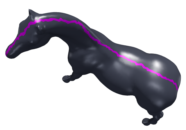
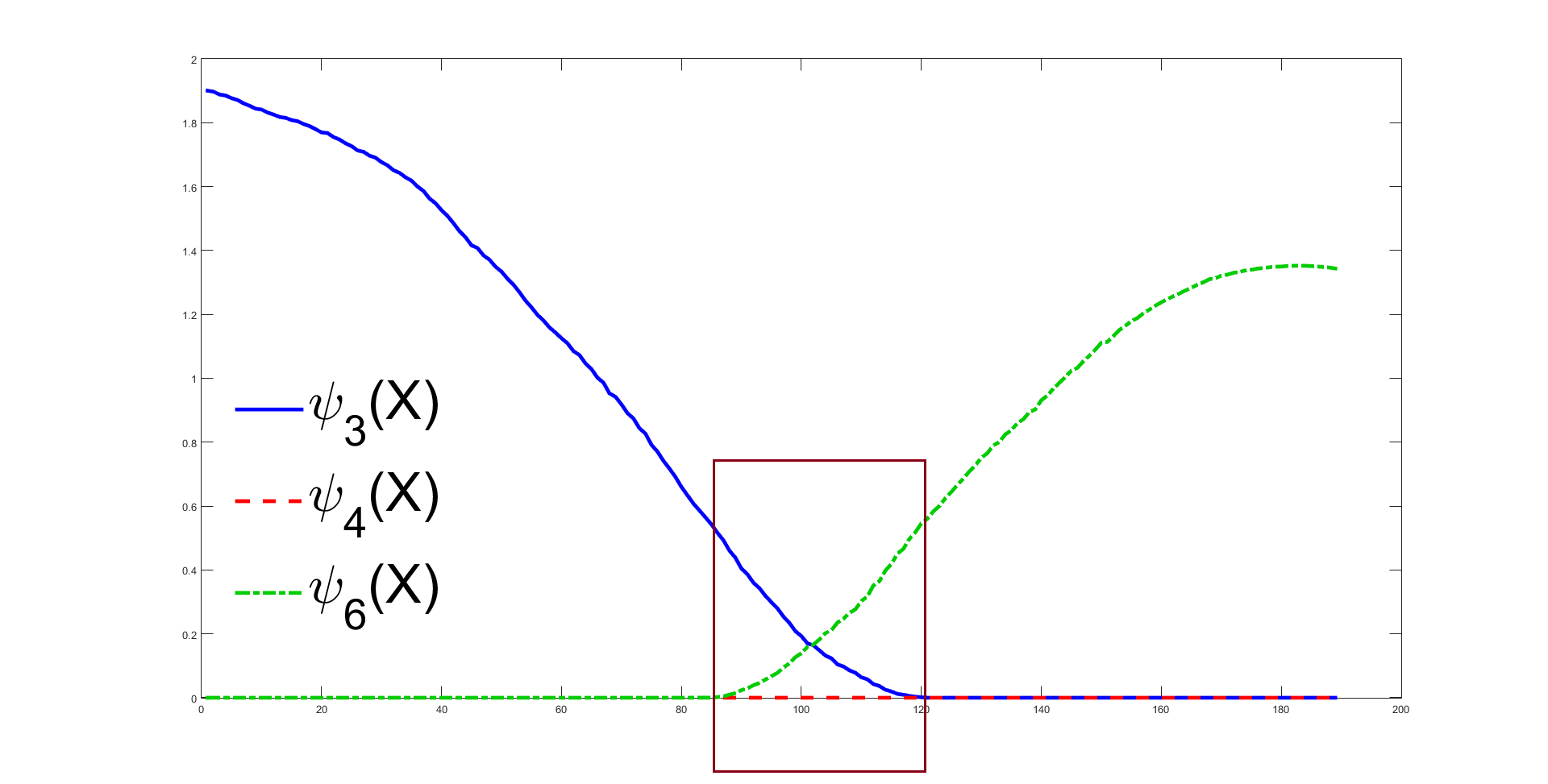
Fig. 4: L_pCMs plotted over the magenta curve on the horse mesh. Over the curve only $\psi_{3}$ and $\psi_{6}$ are non-zero, and the red box shows the band where the supports overlap.

Step 2 ends when the buffers are empty, i.e. all the triangles of M have been assigned to $S$.

An a posteriori procedure approximates the boundaries of the sub-meshes $\{S_{k}\}_{k=1}^{N}$ by smooth spline curves.

Step 3 of Algorithm 1 is applied to finalize the Patch-Based Manifold Partitioning following Definition 2. The refinement is required only for a few patches $\{S_{k}\}_{k=1}^{\bar{N}}$, $\,\bar{N}<N$, with genus greater than zero, and for genus-0 patches with more than two closed-loop boundaries. The refinement is an adaptive process that consists in the re-iteration of Step 1 and Step 2 for every patch $S_{k}$ that needs to be further subdivided, by imposing the initial number of partitions $N=2$.

8 Experimental Results

In this section we describe the experimental results which demonstrate the performance of Algorithm 1. In particular, we first evaluate the performance of Step 1 for the computation of the $L_{p}$ Compressed Modes $\Psi\in{\mathbb{R}}^{n\times N}$, then we illustrate the results of Step 2 and Step 3 for part-/patch-based partitioning, respectively.

Experimental tests were performed on Intel®Core™i7-4720HQ Quad-Core 2.6 GHz machine, with 12 GB/RAM and Nvidia GeForce GTX 860M graphics card in a Windows OS. The code is written in Matlab, and executed without any additional machine support, e.g. parallelization and GPU-based computations.

We tested the proposed method on a set of meshes downloaded from the data repository website http://segeval.cs.princeton.edu, [8]. The dataset represents geometric models with different characteristics in terms of details, level of refinement, and present a medium dense vertex distribution, in particular the number of vertices and triangles of the meshes visualized in the examples are reported in the second and third column of Table 1.

The figures reported in this section were produced by the software ParaView, and its VTK reader. In the examples illustrated we applied a post-process smoothing to the boundaries between the segmented parts $\{S_{k}\}_{k=1}^{N}$ by projecting the boundary vertices onto the cubic spline obtained by least-squares approximation.

8.1 STEP 1: Computing the L_pCMs

The two strategies Step 1a and Step 1b in Algorithm 1, described in section 7, generate the basis functions $\Psi$.

In all the experiments we used a randomized matrix as initial iterate $\Psi^{(0)}$ for the ADMM computation of (12), and we terminated the ADMM iterations as soon as the relative change between two successive iterates satisfies

$$\,err_{\Psi}=\frac{\|\Psi^{(k)}-\Psi^{(k-1)}\|_{F}}{\|\Psi^{(k-1)}\|_{F}}\;{<}\;10^{-3}.$$ (45)

As already observed in [20], where the L₁ penalty term is used, different runs converge to the same set of basis functions, although their ordering might be different. In our experiments the $p$ values were tested in the range $[0.5,0.8]$. However, since small $p$ values affect mainly the efficiency, we decided to set the sparsity parameter $p=0.8$ for all the examples reported.

Figure LABEL:fig:V1_scheme illustrates how Step 1a works when the parameter value $\mu$ is fixed, $\mu=300$. At the first iteration, only two initial quasi-eigenfunctions are computed with the given $\mu$. The control of the local support volume resulted in localizing two legs of the horse mesh, leaving the rest uncovered (highlighted in magenta at the end of the first row). In the second iteration (second row), the space dimension is enlarged ($N=3$), resulting in optimization of $\Psi^{n\times 3}$. The support of the third function $\psi_{3}$ shrinks the uncovered area under the head and neck, leaving just two legs and part of the horse’s body uncovered. The algorithm terminates after five iterations, enlarging the space up to six functions $\psi_{1},\dots,\psi_{6}$ and leaving no more vertices of $M$ uncovered. The result of the last iteration is depicted in the bottom row of Figure LABEL:fig:V1_scheme. Notice that over iterations, the corresponding functions describing the same parts of the mesh retain their order in the set $\Psi$. Due to the randomized initialization, the order in general changes for different runs.

Step $1b$ iteratively recomputes a given number $N$ of basis functions increasing the value of the $\mu$ parameter, thus enlarging the local support at each iteration, until all the vertices of $M$ are covered by at least one function $\psi$. By the way of illustration, in Figure 6 we show the enlargement of the support of $\psi_{5}\in\Psi$ for horse mesh and $\psi_{1}\in\Psi$ for bird mesh, for increasing values of $\mu$ and a fixed basis dimension $N=5$ and $N=4$ respectively. The initial $\mu=8$ is increased by a factor 4 at each iteration. From left to right, the results are shown for $\mu=8$, $\mu=32$, $\mu=128$ and $\mu=512$ .

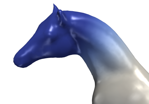
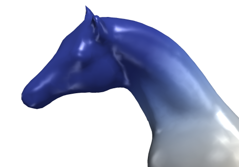
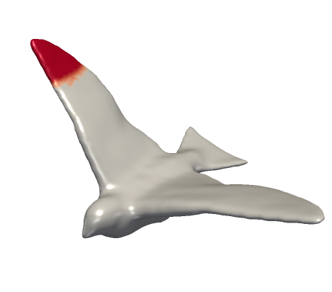
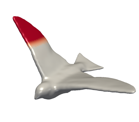
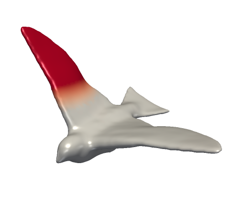
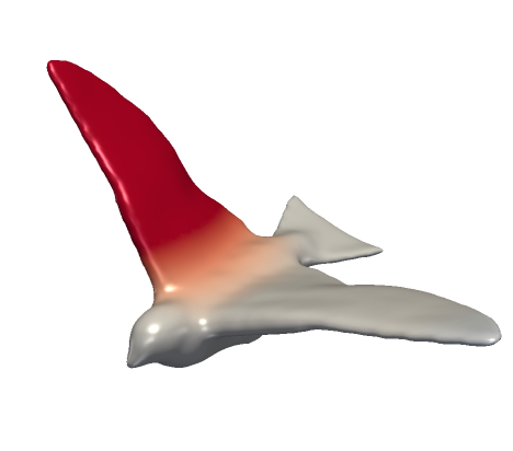
Fig. 6: L_pCM $\psi_{5}$ of $\Psi$ on the horse mesh (top), and $\psi_{1}$ of $\Psi$ on the bird mesh (bottom), both generated for 4 iterations of Step 1b in Algorithm 1. From left to right: enlarging of the support obtained by increasing the parameter $\mu$ for a fixed number of basis functions.

In order to further demonstrate how the L_pCMs localize the details much better than the Laplacian eigenvectors, we consider a synthetic example of an ellipsoid with a growing bump. The ellipsoid’s principal semi-axes are $\{2.5,1.5,1.5\}$ long and it was approximated by triangulated mesh of $|V|=16386$ vertices and $|T|=32768$ triangles. In the top row of Fig. 7 we report the first five non-constant eigenvectors of LBO corresponding to the first five non-zero eigenvalues obtained by solving the generalized eigenvalue problem (3). The eigenvectors present global support and neither the first five nor the rest of the eigenvectors, which are not illustrated here for space constraints, are able to localize the bump. In the bottom rows of Fig. 7 we show the first five L_pCMs for $p=0.8$ and $\mu=125$, for different bump dimensions. In the first and last and row of Fig. 7 the bump dimensions correspond. The compact support $L_{p}$CMs which localize the bumps are highlighted in red boxes.

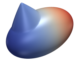
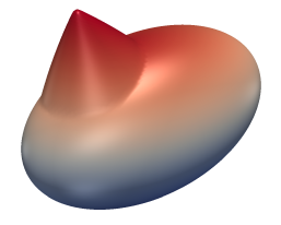
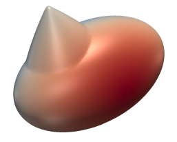
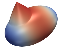
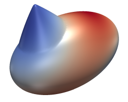
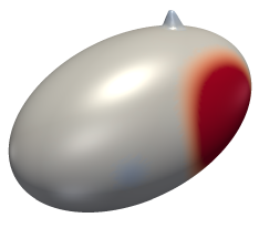
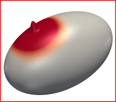
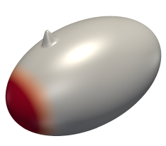
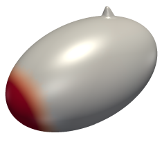
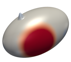
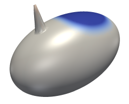
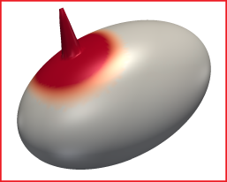
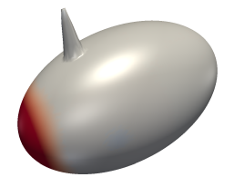
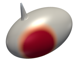
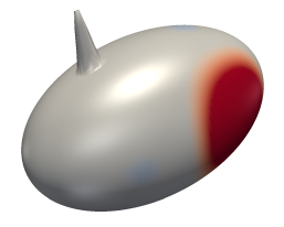
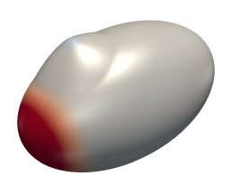
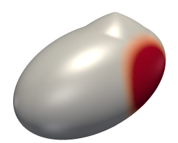
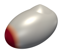
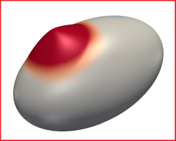
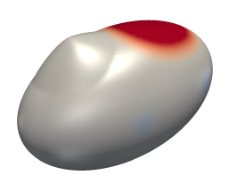
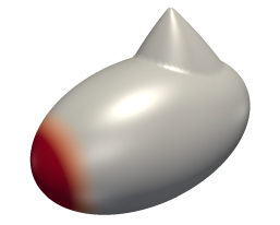
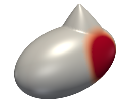
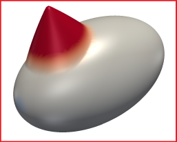
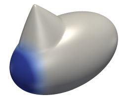
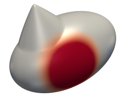
Fig. 7: Comparison of the first five MHB functions and L_pCMs in case of an ellipsoid with a bump. Top row: first 5 non-constant eigenvectors of LBO. Bottom rows: first 5 L_pCMs for different bump dimensions.

We conclude this example presenting an empirical investigation on the numerical convergence of the proposed ADMM-based minimization scheme.

In our formulation (12), we deal with a non-convex orthogonality constraint and non-convex penalty term, i.e. the sparsity-inducing L_p norm. Therefore, the convergence to an optimal solution in the global sense is not guaranteed and we assume that the algorithm converges to at least a local minima, which is still a sufficient result for our application.

At that aim, we investigated the empirical convergence via the relative change of the primal variables, and, following [6], the squared primal residual norm $\|\mathbf{r}\|_{2}^{2}$ which, according to our implementation, is defined as

$$\|\mathbf{r}^{(k)}\|_{2}^{2}=\|\Psi^{(k)}-S^{(k)}\|_{F}^{2}+\|\Psi^{(k)}-E^{(k)}\|_{F}^{2}\,.$$

By the way of illustration, in Figure 8 we report the convergence plots concerning some models used for these examples. The plots in Fig. 8(top) show that the relative errors $err_{\Psi}$ defined in (45) on the ADMM iterates $\Psi^{(k)}$ computed by Step 1 in Algorithm 1, converge to some limit, which indeed indicates convergence of the proposed method (at least to local minimizers), whereas the plots in Fig. 8(bottom) demonstrate that the primal residual norms $\|\mathbf{r}^{(k)}\|_{2}^{2}$ reduce.

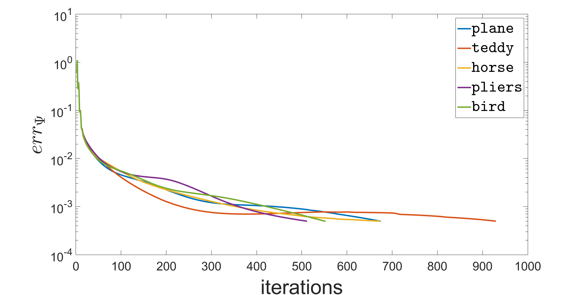
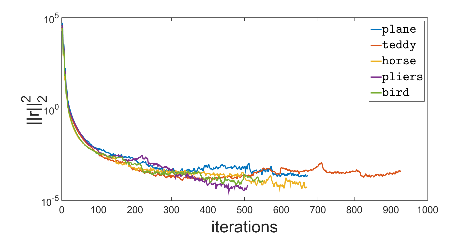
Fig. 8: Relative change of primal variable $\Psi$, $err_{\Psi}$, (top) and primal residual norm $\|\mathbf{r}\|_{2}^{2}$ (bottom) in terms of ADMM iterations.

Table 1: Performance of the mesh segmentation algorithm.

Data set	$|V|$	$|T|$	$K$	$\mu$	STEP 1 (s)	STEP 2 (s)
ant	7038	14072	9	150	9.69	4.79
armadillo	25319	50542	12	140	47.26	13.23
bird	6475	12946	4	300	7.32	4.54
dolphin	7573	15142	7	150	9.40	3.48
fawn	3911	7818	6	150	4.10	2.54
fertility	19994	40000	7	300	26.56	11.57
fish	5121	10238	8	130	7.45	2.11
giraffe	9239	18474	13	130	14.55	3.52
glasses	7407	14810	6	150	7.75	3.36
hand	6607	13210	8	150	8.27	3.32
horse	8078	16152	6	300	9.59	3.81
octopus	5944	11888	9	150	11.14	4.08
plane	7470	14936	7	150	7.54	3.34
pliers	3906	7808	6	130	5.21	2.82
teddy	9548	19092	7	130	12.25	4.53
teddy_2	12831	25658	16	30	22.83	4.47
wolf	4712	9420	7	150	5.94	2.45

8.2 STEP 2: Mesh Segmentation

In Step 2 we apply the region growing algorithm detailed in Section 7 to obtain the partition $S=\{S_{k}\}_{k=1}^{N}$ which represents a decomposition of the mesh into its salient parts. Several examples of mesh segmentation are shown in Figure 9. The number of partitions produced ($N$) is reported on the bottom right of each segmented object.

Details of the datasets are given in Table 1. In particular, for each mesh, we report the number of partitions ($N$), the value of $\mu$ automatically computed by Step 1b, the time in seconds to obtain the L_pCM basis of dimension $N$ in Step 1b, and the time for the mesh segmentation procedure in Step 2 of Algorithm 1.

It is worth mentioning that our segmentation procedure is naive compared with many other spectral segmentation approaches proposed in literature, which are enriched by many heuristic strategies based on curvature criteria or edge detection, which, however, can be easily applied also to our basic algorithm. Nevertheless, the obtained results enhance the good properties of our proposal.

The model fish, illustrated in Fig.10, is considered a particularly difficult challenge since its featured parts (fins, head, tail) are smoothly joined with the rest of the body thus presenting weak boundary strength but good degree of protrusion. In Fig.10 we show a comparison between our L_pCM basis (top left) and the eigenfunctions computed by the truncated spectral decomposition used in [37] (bottom left). The latter is considered the state-of-the-art among the variational methods using spectral analysis.

The salient parts are nicely identified by the L_pCMs using only $N=8$ functions, mimicking the human driven segmentation shown in Fig.10 (right). In [37] the authors claim that even for higher space dimensions their method was not able to localize the salient parts. We notice that in Fig.10 (top row, left) the fish meshes for $\psi_{2}$ and $\psi_{8}$ are visualized upside-down to better show which fins are localized by these supporting functions.

The spectral segmentation results are shown in Fig.11. The starting seeds (left) computed by Step 1 of Algorithm 1 are placed correctly, then the region growing algorithm in Step 2 ends up with the partitioning in Fig.11(middle). On the right of Fig.11 we report the mesh decomposition shown in [37] which has been produced with the help of an edge detection strategy introduced in the variational formulation. A visual insight allows us to observe some defects for both the top fins, on the cluster boundaries which indeed go through the middle of the fins.

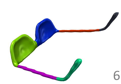
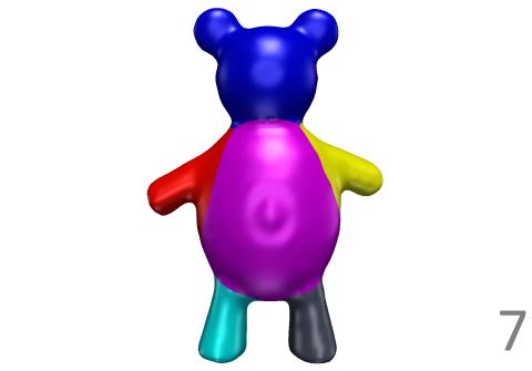
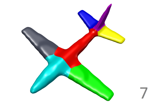
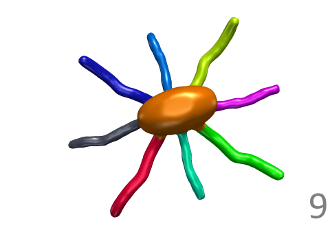
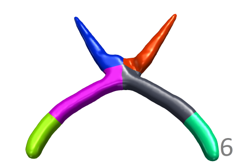
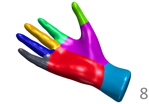
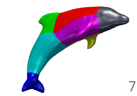
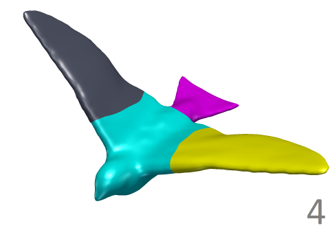
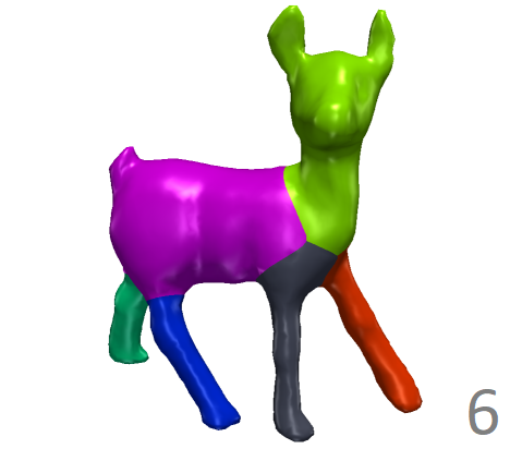
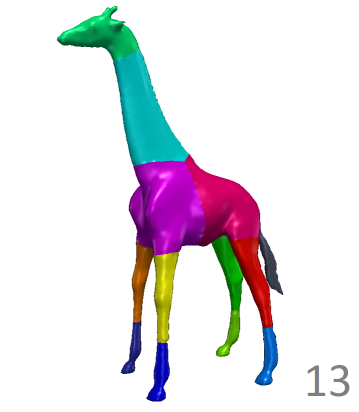
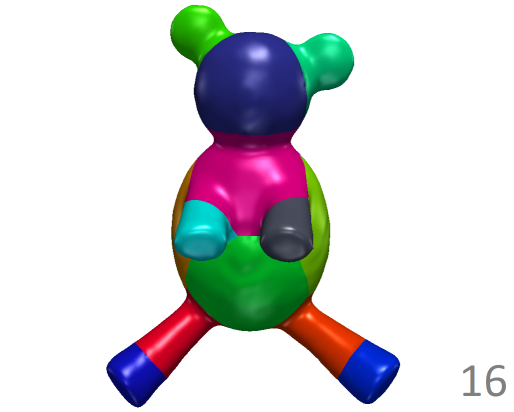
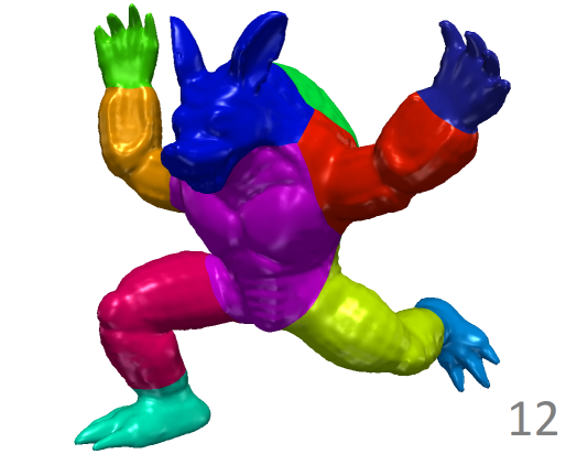
Fig. 9: Mesh partitioning into salient parts obtained in Step 2 of the Algorithm 1.

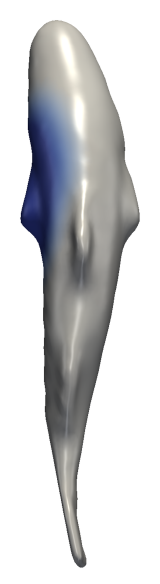
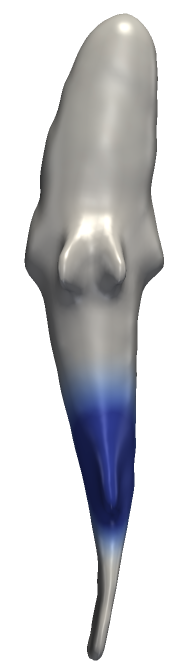
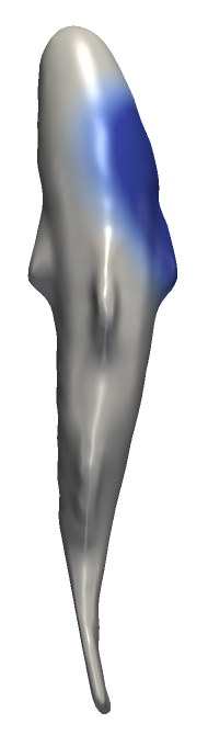
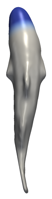
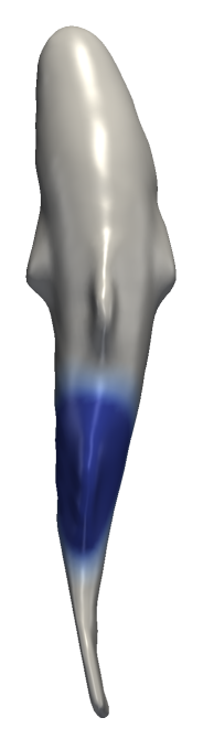
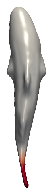
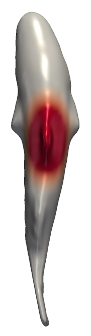
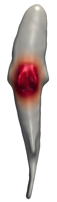
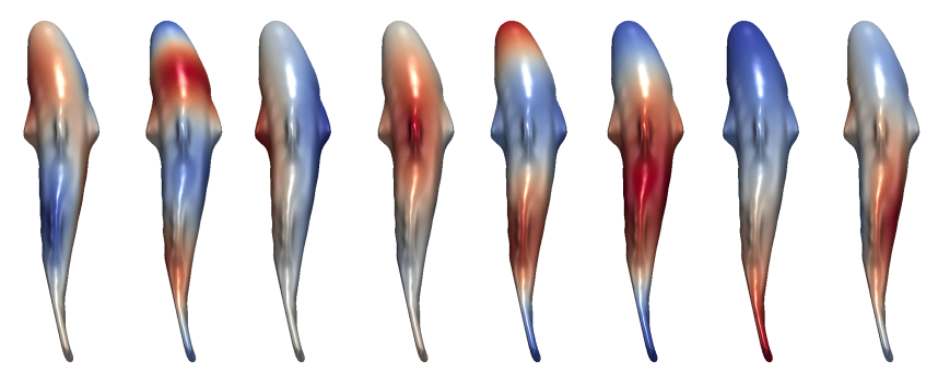
Fig. 10: Supports of the eigenfunctions for the fish mesh: L_pCMs results (top row) and human segmentation (top row, right), eigenfunctions of the affinity matrix proposed in [37] (bottom row).

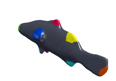
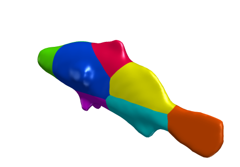
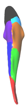
Fig. 11: Segmentation of the fish mesh: seed areas of Step 2(left), mesh segmented by Step 2 (center), and mesh segmentation using [37].

8.3 STEP 3: Patch-based Partitioning

The third step of Algorithm 1 refines the partitioning obtained by Step 2 finalizing a patch-based manifold partitioning, see Def. 2. To this end, we first select from $S$ those parts $S_{k}$ which have genus higher than zero and/or more boundaries, and we re-run Step 1 and Step 2 for each of them until every $S_{k}$ has genus-0 and at most two boundaries.

In Figure 12 we illustrate a few examples of patch-based partitioning resulting from Step 3 (bottom row) in comparison with the mesh partitioning obtained in Step 2 (top row). For all the meshes reported in this figure, just one part (from left to right yellow/red/magenta/red) was further subdivided. The fertility mesh (left), characterized by four holes, represents a closed mesh of higher genus. Also in this case, the algorithm was able to both localize salient parts of the mesh and create a satisfying genus-0 patching.

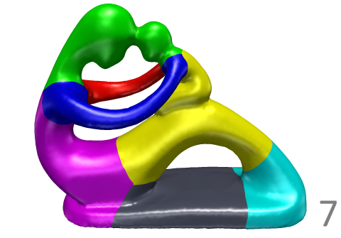
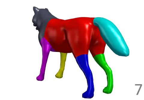
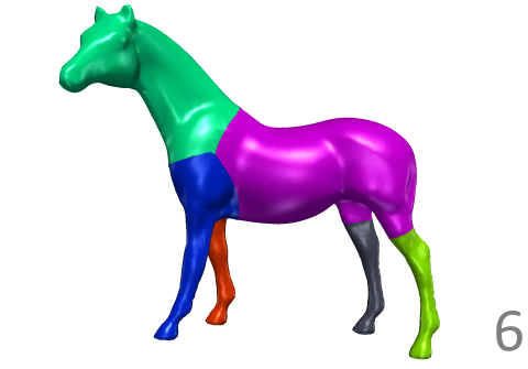
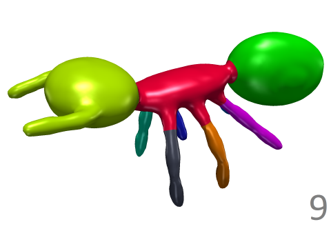
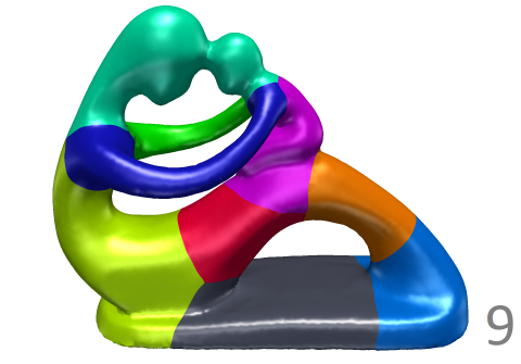
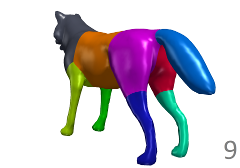
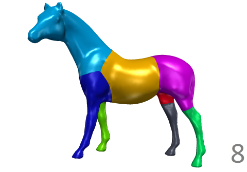
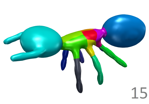
Fig. 12: Mesh segmentation into salient parts obtained by applying Step 2 of Algorithm 1 (top row); patch-based partitioning into genus-0 patches by applying the refinement in Step 3 (bottom row).

9 Conclusions

In this paper, we proposed a sparsity-promoting variational method to produce compressed functions L_pCMs which are quasi-eigenfunctions of the Laplacian operator. We proved that the generated functions are highly localized in space and the size of their support depends on the sparsity parameter $p$ and on the penalty parameter $\mu$. An Augmented Lagrangian method was applied to solve this non-convex non-differentiable optimization problem, yielding an iterative algorithm with efficient solutions to subproblems. This compact support basis proves to be very useful for spectral shape processing. In particular, we proposed a unified method for shape partitioning that can be applied to both mesh segmentation and patch-based partitioning, which is based on a more restrictive requirement with respect to mesh segmentation. In mesh segmentation each sub-mesh represents a meaningful part of the object from a human perception point of view. In patch-based partitioning instead each part is characterized by genus-0 topology which easily allows it to be parametrized. Our proposed Algorithm 1, thanks to the compactness of the generated L_pCM basis, well performs on typical mesh partitioning problems, but it still has some limitations. We have not obtained a convergence proof, which is probably very challenging due to the non-convexity of the problem. Besides, in our tests, we found out that the parameter $p$ affects the algorithm efficiency. When $p$ is very small, for example $p<0.4$, our algorithm is slow. Acceleration techniques for strong sparsity requirements remain to be designed and they will be considered in future work.

APPENDIX

Proof of Theorem9.

Proof.

The proof is decomposed in four steps.
Step 1:
We first derived the Euler-Lagrange equations for (5). For any fuction $u$, let s(u) denote an element of subdifferential of $\left|u\right|^{p}$, that is:

$$s(u)=sign(u)\cdot p\cdot\left|u\right|^{p-1}.\;$$ (46)

The solutions of (5) are weak solutions of the following system of nonlinear boundary value problem:

$$\frac{1}{\mu}s(\psi_{i})-2\lambda_{ii}\psi_{i}-\Delta\psi_{i}-\sum_{j\neq i}\lambda_{ij}\psi_{j}=0,\quad i=1,..,N\;\mbox{on}\quad\Omega$$ (47)

where $\lambda_{ij}$, with $\lambda_{ij}=\lambda_{ji}$ are Lagrange multipliers corresponding to orthonormality constraints:

$$\int_{\Omega}{\psi_{i}^{2}dx}=1\quad\mbox{and}\quad\int_{\Omega}{\psi_{i}\psi_{j}dx}=0,\quad\mbox{for}\quad i,j=1,...,N,\;j\neq i.$$ (48)

Step 2: Upper bounds for $\lambda_{ii}$, $\|\psi_{i}\|_{p}^{p}$ and $\|\nabla\psi_{i}\|_{2}$
For each $i$ multiply both sides of equation (47) by $\psi_{i}(x)$ and integrate over domain $\Omega$:

$$\int_{\Omega}{\frac{1}{\mu}s(\psi_{i})\psi_{i}dx}-2\lambda_{ii}\int_{\Omega}{\psi_{i}\psi_{i}dx}-\int_{\Omega}{\Delta\psi_{i}\psi_{i}dx}-\sum_{j\neq i}\lambda_{ij}\int_{\Omega}{\psi_{i}\psi_{j}dx}=0.$$ (49)

By using orthonormality conditions (48), we can rewrite the above equation as:

$$\int_{\Omega}{\frac{1}{\mu}s(\psi_{i})\psi_{i}dx}-2\lambda_{ii}-\int_{\Omega}{\Delta\psi_{i}\psi_{i}dx}=0$$ (50)

that, using integration by parts and zero boundary conditions on $\Omega$, implies that

$$\int_{\Omega}{\frac{1}{\mu}s(\psi_{i})\psi_{i}dx}-2\lambda_{ii}+\int_{\Omega}{\left|\nabla\psi_{i}\right|^{2}dx}=0$$ (51)

and then

$$\lambda_{ii}=\frac{1}{2\mu}\int_{\Omega}{s(\psi_{i})\psi_{i}dx}+\frac{1}{2}\int_{\Omega}{\left|\nabla\psi_{i}\right|^{2}dx}.$$ (52)

By using definition (46), relation (52) can be reformulated as:

$$\lambda_{ii}=\frac{1}{2\mu}\int_{\Omega}{p\left|\psi_{i}\right|^{p}dx}+\frac{1}{2}\int_{\Omega}{\left|\nabla\psi_{i}\right|^{2}dx}$$ (53)

From Proposition 1, we know that the first compressed mode $\psi$ has support whose volume satisfy (6). It follows that for $\mu$ sufficiently small and $0<p<1$, the $N$ disjoint copies (i.e. translates) of $\psi$ can be placed in $\Omega$, and these $N$ functions are a solution for problem (5). Therefore, in view of Proposition 1, there exist $\mu_{0}$ (depending on values of $p$,$N$, and $d$) such that for $\mu<\mu_{0}$:

$$\sum_{i=1}^{N}\int_{\Omega}{\frac{1}{\mu}\left|{\psi_{i}}\right|^{p}dx}+\sum_{i=1}^{N}\frac{1}{2}\int_{\Omega}{\left|\nabla{\psi_{i}}\right|^{2}dx}\leq m(\Omega)^{\frac{1}{p}-1}C_{1}N\mu^{-\frac{4}{4+d}}.$$ (54)

Because each of the summands in the left hand side of above inequality is positive, there exist constant $C_{2}$ (depending on $d$ and $N$) such that for $\mu<\mu_{0}$,

$$\int_{\Omega}{\frac{1}{\mu}\left|{\psi_{i}}\right|^{p}dx}\leq m(\Omega)^{\frac{1}{p}-1}C_{2}\mu^{-\frac{4}{4+d}}\quad\mbox{and}\quad\int_{\Omega}{\left|\nabla{\psi_{i}}\right|^{2}dx}\leq m(\Omega)^{\frac{1}{p}-1}C_{2}\mu^{-\frac{4}{4+d}}.$$ (55)

Moreover, replacing the above inequalities into (53), it follows that there exist a constant $C_{3}$ (depending on $d$, $N$ and $p$), such that for $\mu<\mu_{0}$

$$\left|\lambda_{ii}\right|<p\frac{C_{2}}{2}\mu^{-\frac{4}{4+d}}m(\Omega)^{\frac{1}{p}-1}+p\frac{C_{2}}{2}\mu^{-\frac{4}{4+d}}m(\Omega)^{\frac{1}{p}-1}<C_{3}\mu^{-\frac{4}{4+d}}m(\Omega)^{\frac{1}{p}-1}.$$ (56)

Step 3: Upper bounds for $\lambda_{ij}^{\prime}s$.
Fix $i$. For $k\neq i$, multiply both sides of equation (47) by $\psi_{k}(x)$ and integrate over $\Omega$:

$$\int_{\Omega}{\left(\frac{1}{\mu}s(\psi_{i})\psi_{k}-2\lambda_{ii}\psi_{i}\psi_{k}-\Delta\psi_{i}\psi_{k}-\sum_{j\neq i}\lambda_{ij}\psi_{j}\psi_{k}\right)dx}=0$$ (57)

which, using orthonormality condition (48) and integration by parts, implies that:

$$\frac{1}{\mu}\int_{\Omega}{s(\psi_{i})\psi_{k}dx}+\int_{\Omega}{(\nabla\psi_{i})(\nabla\psi_{k})dx}-\lambda_{ik}=0.$$ (58)

Therefore

$$\lambda_{ik}=\frac{1}{\mu}\int_{\Omega}{s(\psi_{i})\psi_{k}dx}+\int_{\Omega}{(\nabla\psi_{i})(\nabla\psi_{k})dx}.$$ (59)

By using relation (46), we have

$$\left|\frac{1}{\mu}\int_{\Omega}{s(\psi_{i})\psi_{k}dx}\right|\leq\frac{1}{\mu}\int_{\Omega}{\left|s(\psi_{i})\psi_{k}\right|dx}=\frac{p}{\mu}\int_{\Omega}{\left|\psi_{i}\right|^{p-1}\left|\psi_{k}\right|dx}=\frac{p}{\mu}\int_{\Omega}{\left|\psi_{i}\right|^{p}\frac{\left|\psi_{k}\right|}{\left|\psi_{i}\right|}dx}.$$ (60)

Since $\left|\psi_{i}\right|^{p}$ does not change sign on $\Omega$, by the First Mean Value Theorem for Integrals, there exists $\xi\in\Omega$, with $\psi_{i}(\xi)\neq 0$, such that, if we set $M=\frac{\left|\psi_{k}(\xi)\right|}{\left|\psi_{i}(\xi)\right|}$, it follows that

$$\frac{p}{\mu}\int_{\Omega}{\left|\psi_{i}\right|^{p}\frac{\left|\psi_{k}\right|}{\left|\psi_{i}\right|}dx}=M\frac{p}{\mu}\int_{\Omega}{\left|\psi_{i}\right|^{p}dx}.$$

Making use of (55), we conclude that

$$\left|\frac{1}{\mu}\int_{\Omega}{s(\psi_{i})\psi_{k}dx}\right|\leq pMm(\Omega)^{\frac{1}{p}-1}C_{2}\mu^{-\frac{4}{4+d}}.$$ (61)

Finally, using Cauchy-Schwarz and equation (55),

$$\left|\int_{\Omega}{(\nabla\psi_{i})(\nabla\psi_{k})dx}\right|\leq\left(\int_{\Omega}{\left|\nabla\psi_{i}\right|^{2}dx}\right)^{\frac{1}{2}}\left(\int_{\Omega}{\left|\nabla\psi_{k}\right|^{2}dx}\right)^{\frac{1}{2}}<\\ (m(\Omega)^{\frac{1}{p}-1}C_{2}\mu^{-\frac{4}{4+d}})^{\frac{1}{2}}(m(\Omega)^{\frac{1}{p}-1}C_{2}\mu^{-\frac{4}{4+d}})^{\frac{1}{2}}\,=\,m(\Omega)^{\frac{1}{p}-1}C_{2}\mu^{-\frac{4}{4+d}}.$$ (62)

Substituting the two upper bounds given in (61) and (62) into equation (59), we have for $\mu<\mu_{0}$

$$\left|\lambda_{ik}\right|<pMm(\Omega)^{\frac{1}{p}-1}C_{2}\mu^{-\frac{4}{4+d}}+m(\Omega)^{\frac{1}{\tilde{p}}-1}C_{2}\mu^{-\frac{4}{4+d}}=\\ m(\Omega)^{\frac{1}{p}-1}C_{2}\mu^{-\frac{4}{4+d}}(pM+1)<C_{4}m(\Omega)^{\frac{1}{\tilde{p}}-1}\mu^{-\frac{4}{4+d}}$$ (63)

where $C_{4}$ depends on $N$, $M$, $p$ and $\mu$.

Step 4: Bounding the volume of the support $\psi_{i}$’s
For each $i$ multiply both sides of equation (47) by $\frac{1}{p}sign(\psi_{i})\left|\psi_{i}\right|^{1-p}$ and integrate over domain $\Omega$:

$$\frac{1}{\mu}\left|supp(\psi_{i})\right|-\frac{2}{p}\lambda_{ii}\int_{\Omega}{\left|\psi_{i}\right|^{2-p}dx}-\frac{1}{p}\int_{\Omega}{\Delta\psi_{i}sign(\psi_{i})\left|\psi_{i}\right|^{1-p}dx}-\frac{1}{p}\sum_{j\neq i}\lambda_{ij}\int_{\Omega}{\psi_{j}sign(\psi_{i})\left|\psi_{i}\right|^{1-p}dx}=0,$$ (64)

namely,

$$\frac{1}{\mu}\left|supp(\psi_{i})\right|=\\ \left|\frac{2}{p}\lambda_{ii}\int_{\Omega}{\left|\psi_{i}\right|^{2-p}dx}+\frac{1}{p}\int_{\Omega}{\Delta\psi_{i}sign(\psi_{i})\left|\psi_{i}\right|^{1-p}dx}+\frac{1}{p}\sum_{j\neq i}\lambda_{ij}\int_{\Omega}{\psi_{j}sign(\psi_{i})\left|\psi_{i}\right|^{1-p}dx}\right|\leq\\ \left|\frac{2}{p}\lambda_{ii}\int_{\Omega}{\left|\psi_{i}\right|^{2-p}dx}+\frac{1}{p}\int_{\Omega}{\Delta\psi_{i}sign(\psi_{i})\left|\psi_{i}\right|^{1-p}dx}\right|+\left|\frac{1}{p}\sum_{j\neq i}\lambda_{ij}\int_{\Omega}{\psi_{j}sign(\psi_{i})\left|\psi_{i}\right|^{1-p}dx}\right|.$$ (65)

Define

$$\Omega^{+}=\left\{x\in\Omega:\psi_{i}(x)>0\right\}$$

and

$$\Omega^{-}=\left\{x\in\Omega:\psi_{i}(x)<0\right\}.$$

According to Green’s formula

$$\int_{\Omega^{+}}{\Delta\psi_{i}dx}=\int_{\partial\Omega^{+}}{\frac{\partial\psi_{i}}{\partial\nu}dS}\leq 0,$$

where $\nu$ is outward pointing unit normal vector along $\partial\Omega^{+}$. Since $\psi$ is positive in $\Omega^{+}$ and becomes zero on $\partial\Omega^{+}$, the right-hand side of the above expression is not positive.
With a similar argument, we have that

$$\int_{\Omega^{-}}{\Delta\psi_{i}dx}=\int_{\partial\Omega^{-}}{\frac{\partial\psi_{i}}{\partial\nu}dS}\geq 0.$$

Hence, since $\left|\psi_{i}\right|^{1-p}\geq 0$ $\forall i$, it follows that:

$$\int_{\Omega}{\Delta\psi_{i}sign(\psi_{i})\left|\psi_{i}\right|^{1-p}dx}=\int_{\Omega^{+}}{\Delta\psi_{i}\left|\psi_{i}\right|^{1-p}dx}-\int_{\Omega^{-}}{\Delta\psi_{i}\left|\psi_{i}\right|^{1-p}dx}\leq 0.$$ (66)

Using inequality (66), (65) can be rewritten as:

$$\frac{1}{\mu}\left|supp(\psi_{i})\right|\leq\left|\frac{2}{p}\lambda_{ii}\int_{\Omega}{\left|\psi_{i}\right|^{2-p}dx}\right|+\left|\frac{1}{p}\sum_{j\neq i}\lambda_{ij}\int_{\Omega}{\left|\psi_{j}\right|\left|\psi_{i}\right|^{1-p}dx}\right|\leq\\ \frac{2}{p}|\lambda_{ii}|\int_{\Omega}{\left|\psi_{i}\right|^{2-p}dx}+\frac{1}{p}\sum_{j\neq i}|\lambda_{ij}|\int_{\Omega}{\left|\psi_{j}\right|\left|\psi_{i}\right|^{1-p}dx}\leq\\ \frac{2}{p}|\lambda_{ii}|\int_{\Omega}{\left|\psi_{i}\right|\left|\psi_{i}\right|^{1-p}dx}+\frac{1}{p}\sum_{j\neq i}|\lambda_{ij}|\int_{\Omega}{\left|\psi_{j}\right|\left|\psi_{i}\right|^{1-p}dx}$$ (67)

We set $\tilde{p}=1-p$, $0<\tilde{p}<1$ , for $0<p<1$.

$$\frac{1}{\mu}\left|supp(\psi_{i})\right|\leq\frac{2}{p}|\lambda_{ii}|\int_{\Omega}{\left|\psi_{i}\right|\left|\psi_{i}\right|^{\tilde{p}}dx}+\frac{1}{p}\sum_{j\neq i}|\lambda_{ij}|\int_{\Omega}{\left|\psi_{j}\right|\left|\psi_{i}\right|^{\tilde{p}}dx}$$ (68)

Since $\left|\psi_{i}\right|^{\tilde{p}}$ does not change sign on $\Omega$, by the First Mean Value Theorem for Integrals, there exist $\xi,\eta\in\Omega$ such that, if we set $\bar{M}=\left|\psi_{i}(\xi)\right|$ and $\tilde{M}=\left|\psi_{j}(\eta)\right|$, relation (68) can be rewritten as:

$$\frac{1}{\mu}\left|supp(\psi_{i})\right|\leq\frac{2}{p}\bar{M}|\lambda_{ii}|\int_{\Omega}{\left|\psi_{i}\right|^{\tilde{p}}dx}+\frac{1}{p}\sum_{j\neq i}\tilde{M}|\lambda_{ij}|\int_{\Omega}{\left|\psi_{i}\right|^{\tilde{p}}dx}.$$ (69)

By using (55), (56),(63), then (69) becomes:

$$\frac{1}{\mu}\left|supp(\psi_{i})\right|\leq\frac{2}{p}\bar{M}C_{3}m(\Omega)^{\frac{1}{p}-1}\mu^{-\frac{4}{4+d}}m(\Omega)^{\frac{1}{1-p}-1}C_{2}\mu^{-\frac{4}{4+d}+1}+\\ \frac{1}{p}(N-1)\tilde{M}C_{4}m(\Omega)^{\frac{1}{p}-1}\mu^{-\frac{4}{4+d}}m(\Omega)^{\frac{1}{1-p}-1}C_{2}\mu^{-\frac{4}{4+d}+1}\\ \leq C_{5}\mu^{-\frac{8}{4+d}+1}m(\Omega)^{\frac{1}{p(1-p)}-2}$$ (70)

where $C_{5}$ depends on $N$ and $p$. ∎

References

- [1] A. Agathos, I. Pratikakis, S. Perantonis, N. Sapidis and P. Azariadis, 3D Mesh Segmentation Methodologies for CAD applications Computer-Aided Design & Applications, Vol. 4(6), pp. 827–841, 2007.
- [2] M. Attene, S. Katz, M. Mortara, G. Patane, M. Spagnuolo, and A. Tal, Mesh Segmentation - A Comparative Study, In Proceedings of the IEEE International Conference on Shape Modeling and Applications 2006 (SMI ’06), IEEE Computer Society, Washington, DC, USA, 7, 2006.
- [3] F. Barekat, On the Consistency of Compressed Modes for Variational Problems Associated with the Schrödinger Operator, SIAM Journal on Mathematical Analysis, Vol. 46(5), pp. 3568–3577, 2014.
- [4] F. Barekat, R. Caflish and S. Osher, On the Support of Compressed Modes, CAM Reports, 2014.
- [5] H. Benhabiles, G. Lavoué, J.-P. Vandeborre, and M. Daoudi, Learning boundary edges for 3D-mesh segmentation, Comput. Graph. Forum, Vol. 30(8), pp. 2170–2182, 2011.
- [6] S. Boyd, N. Parikh, E. Chu, B. Peleato, and J. Eckstein, Distributed Optimization and Statistical Learning via the Alternating Direction Method of Multipliers, Foundations and Trends in Machine Learning, Vol. 3(1), pp. 1–122, 2011.
- [7] M. Chahhou, L. Moumoun, M. El Far, and T. Gadi, Segmentation of 3D Meshes Using p-Spectral Clustering, IEEE transactions on pattern analysis and machine intelligence, Vol. 36(8), pp. 1687–1693, 2014.
- [8] X. Chen, A. Golovinskiy, T. Funkhouser, A Benchmark for 3D Mesh Segmentation, ACM Trans. Graph. Vol. 28(3), pp. 73:1–73:12, 2009.
- [9] M. S. Floater and K. Hormann. Surface parameterization: a tutorial and survey. In N. A. Dodgson, M. S. Floater, and M. A. Sabin, editors, Advances in Multiresolution for Geometric Modelling, Mathematics and Visualization, pp. 157–186, Springer, Berlin, Heidelberg, 2005.
- [10] Y. Gao, P. G. Menon, and Y. Zhang, 3D shape comparison of cardiac geometries using a Laplace spectral-shape-matching approach. CMBBE: Imaging & Visualization, Vol. 4, pp. 86–97, 2016.
- [11] J. C. Gower, G.B. Dijksterhuis, Procrustes Problems, Oxford University Press, (2004).
- [12] M. Huska, S.Morigi, Sparsity-inducing variational shape partitioning, Electronic Transactions on Numerical Analysis, Vol. 46, pp. 36–54, 2017.
- [13] E. Kalogerakis, A. Hertzmann, and K. Singh, Learning 3D mesh segmentation and labeling, ACM Trans. Graph., Vol. 29(4), pp. 102:1–102:12, 2010.
- [14] R. Lai, S. Osher, A Splitting Method for Orthogonality Constrained Problems Journal of Scientific Computing, Vol. 58(2), pp. 431-–449, 2014.
- [15] A. Lanza, S. Morigi, F. Sgallari, Constrained TVp-L2 model for Image Restoration, Journal of Scientific Computing (JOMP), Vol. 68(1), pp. 64–91, 2016.
- [16] B. Lévy and H.R. Zhang, Spectral mesh processing, In ACM SIGGRAPH 2010 Courses (SIGGRAPH ’10). ACM, New York, NY, USA, 2010.
- [17] H. Lin, W. Chen, H. Bao, Adaptive patch-based mesh fitting for reverse engineering, Computer-Aided Design, Vol. 39(12), pp. 1134–1142, 2007.
- [18] R. Liu, H. Zhang. Segmentation of 3d meshes through spectral clustering. In Computer Graphics and Applications, PG 2004, Proceedings, 12th Pacific Conference on (Oct 2004), pp. 298–-305, 2004.
- [19] D. Mejia, O. Ruiz-Salguero, C. A. Cadavid, Spectral-based mesh segmentation, International Journal on Interactive Design and Manufacturing (IJIDeM):1955-2505, pp. 1–12, 2016.
- [20] T. Neumann, K. Varanasi, C. Theobalt, M. Magnor, and M. Wacker, Compressed Manifold Modes for Mesh Processing, Computer Graphics Forum (Proc. of Symposium on Geometry Processing SGP), Eurographics Association, Vol. 33(5), pp. 35–44, 2014.
- [21] V. Ozoliņš, R. Lai, R. Caflisch, and S. Osher, Compressed Modes for Variational Problems in Mathematics and Physics, Proceedings of the National Academy of Sciences 110(46):18368-18373, 2013.
- [22] G. Patanè, M. Spagnuolo, B. Falcidieno, Families of cut-graphs for bordered meshes with arbitrary genus, Graphical Models, Vol. 69 (2), pp. 119–138, 2007.
- [23] G. Patanè, M. Spagnuolo and B. Falcidieno, Para-Graph: Graph-Based Parameterization of Triangle Meshes with Arbitrary Genus, Computer Graphics Forum, Vol. 23(4), pp. 783–797, 2004.
- [24] U. Pinkall and K. Polthier, Computing Discrete Minimal Surfaces and Their Conjugates, Experimental Mathematics, 2, pp. 15–36, 1993.
- [25] M. Reuter, F.-E. Wolter, and N. Peinecke, Laplace-spectra as fingerprints for shape matching, In Proceedings of the 2005 ACM symposium on Solid and physical modeling (SPM ’05), ACM, New York, NY, USA, pp. 101–106, 2005.
- [26] P. H. Schonemann, On the Formal Differentiation of Traces and Determinants, Multivariate Behavioral Research, Vol. 20(2), pp. 113–139, 1985.
- [27] A. Shamir, A survey on mesh segmentation techniques, Computer Graphics Forum, Vol. 27(6), pp. 1539–1556, 2008.
- [28] R. Song, Y. Liu, R. R. Martin, and P. L. Rosin, Mesh saliency via spectral processing, ACM Trans. Graph, 33, 1, Article 6, 6:1–6:17, 2014.
- [29] D. Steiner and A. Fischer, Cutting 3D freeform objects with genus-n into single boundary surfaces using topological graphs, In Symposium on Solid Modeling and Applications, pp. 336–343, 2002.
- [30] P. Theologou, I. Pratikakis, T. Theoharis, A comprehensive overview of methodologies and performance evaluation frameworks in 3D mesh segmentation, Computer Vision and Image Understanding, Volume 135, pp. 49–82, 2015.
- [31] P. Theologou, Pratikakis I, Theoharis T., Unsupervised Spectral Mesh Segmentation Driven by Heterogeneous Graphs, IEEE Trans Pattern Anal Mach Intell., Vol. 39(2), pp. 397–410, 2017.
- [32] B. Vallet, B. Lévy, Spectral geometry processing with manifold harmonics, Computer Graphics Forum 27 (2), pp. 251–260, 2008.
- [33] T. Varady, Automatic Procedures to Create CAD Models from Measured Data Computer-Aided Design and Applications 5(5):577-588, 2013.
- [34] H. Wang, T. Lu, O. K.-C. Au, and C.-L. Tai, Spectral 3D mesh segmentation with a novel single segmentation field. Graph. Models 76, 5 (September 2014), pp. 440–456, 2014.
- [35] D.-M. Yan, W. Wang, Y. Liuc, Z. Yang, Variational Mesh Segmentation via Quadric Surface Fitting, Computer-Aided Design 44(11), pp. 1072–1082, 2012.
- [36] K. Yin, S. Osher, On the Completeness of the Compressed Modes in the Eigenspace, UCLA CAM Report, pp. 13–62, 2013.
- [37] J. Zhang, J. Zheng, C. Wu, and J. Cai, Variational mesh decomposition, ACM Trans. Graph., Vol. 31/3, pp. 21:1–21:14, 2012.
- [38] W. Zuo, D. Meng, L. Zhang, X. Feng, and D. Zhang, A Generalized Iterated Shrinkage Algorithm for Non-convex Sparse Coding, International Conference of Computer Vision (ICCV), pp. 217–224, 2013.
Acknowledgements
We would like to thank the referees for comments that lead to improvements of the presentation. Research was supported in part by the National Group for Scientific Computation (GNCS-INDAM), Research Projects 2015.