A Rigorous Analysis of Least Squares Sine Fitting Using Quantized Data: the Random Phase Case

Abstract

This paper considers least–square based estimation of the amplitude and square amplitude of a quantized sine wave, done by considering random initial record phase. Using amplitude– and frequency–domain modeling techniques, it is shown that the estimator is inconsistent, biased and has a variance that may be underestimated if the simple model of quantization is applied. The effects of both sine wave offset values and additive Gaussian noise are taken into account. General estimator properties are derived, without making simplifying assumptions on the role of the quantization process, to allow assessment of measurement uncertainty, when this least–square procedure is used.

I Introduction

When assessing the properties of systems subject to quantized input data, the simple noise model of quantization [1] may be used to obtain results quickly. However, it may also lead to severe approximations when necessary hypotheses for its application do not hold true. This model is based on the assumption that the effects of quantization may be represented by a source of uncorrelated uniformly distributed random variables. Practitioners can discriminate among applicability situations, on the basis of their technical intuition. Nevertheless, only sound mathematical modeling can compensate for lack of insight into the properties of complex algorithms based on quantized data.

I-A Least Squares Estimation and Quantization

Parametric estimation based on Least Squares (LS), is widely used as an all–purpose estimation technique, with applications in many engineering domains. This is the case, for instance, of the the $3$– or $4$–parameter sine fit method described in [2], used to estimate the meaningful parameters of a sampled sine wave, when testing Analog-to-Digital Converters (ADC). In practice, measurement data are almost always obtained by converting analog signals in the digital domain, by means of an ADC. As a consequence, they rarely satisfy the conditions for the LS approach to be considered optimal [3][4]. Conversely, the quantization process will result in estimator properties, that can not easily be analyzed, if the simple noise model of quantization is adopted. This latter simplification can ease the evaluation of order of magnitudes in assessing the estimator bias and variance. However, it can be misleading if precise measurements and accurate assessments of corresponding uncertainties are necessary. This occurs in metrology and in many areas of electrical engineering where quantization plays a role. In fact, it is well known that this model breaks down, even when very simple input signals enter the processing chain, such as a direct current value. Nevertheless, engineers often rely on this approximation, and trade accuracy in the analysis of considered systems for speed and ease in the solution of associated calculations. Also estimations based on a metrological–sound approach can not rely on simplified procedures but must include all available knowledge needed to provide bounds on estimation errors. This applies, for instance, when ADCs are tested using sine waves as source signals. The estimation of the sine sine wave amplitude needed to estimate other meaningful parameters, e.g. number of effective bits, is done by using the quantized data at the ADC output [2].

This work shows that the simple model fails to predict both the bias and the variance of the LS–based estimator of the amplitude and square amplitude of a quantized sine wave. By adopting several modeling techniques it also shows how to include the effect of quantization into calculations, without making simplifying assumptions.

The used analytical tools may serve as a fully developed example about how solving similar problems, when analogous measuring conditions apply.

I-B The State–of–the–Art

Previous work on the characterization of a LS–based estimator applied to the parameters of a sine wave subject to Gaussian noise, has been published recently in [5][9]. Reference [5] contains a detailed analysis of the LS–based estimator properties, when assuming the input sine wave corrupted by additive Gaussian noise. It is shown that noise contributes to estimation bias, also in absence of quantization. In [9], the author takes [5] as a starting point and extends its results by using alternative derivations and by adding simple closed–form asymptotics, valid for small errors. This work broadens the analysis to the case in which the sine wave is quantized before amplitude estimation is performed. The same topic is addressed in [10] where, through simulations, a description of the LS–based estimator bias is obtained, under the assumption of quantized data, and a modified technique for bias reduction is illustrated. Relevant results to this work are presented in [6] where the definition of the effective number of bits (ENOB) in an ADC is processed to account for deviations in testing signal offset and amplitude. Previous work on the same subject was carried out in [7], where again the definition of ENOB was discussed in relation to the properties of the quantization error characteristics of a noiseless quantizer and a new analytical method for its assessment was proposed.

I-C The Main Results in this Paper

In this paper, at first a practical example is given to motivate the necessity for this analysis. Then, the properties of the estimator of the square amplitude of a quantized sine wave are analyzed, under the assumption of randomly distributed initial record phase. This is a choice of practical interest, because phase synchronization is not always feasible in the engineering practice, when repeated or reproduced measurements results are needed. In these cases, algorithms are applied on quantized data, without knowledge of the initial record phase. Thus, their properties can be analyzed by assuming this phase uniformly distributed in the interval $[0,2\pi)$. This assumption is relevant to the analysis of the estimator properties prior to executing measurements. When an experiment is performed, a realization of the random variable modeling the initial record phase occurs. From that moment on, the sequence has a deterministic behavior. Thus, results presented here, serve to understand what to expect before taking measurements and how to interpret results when comparing estimations obtained when sampling is not synchronized.

As it is still customary, to use the noise model of quantization to produce estimates of error mean values and variances, the results presented in this paper will serve two major purposes: warn against the unconditional application of this model, as it can lead to underestimates of measurement uncertainties and show how to use various mathematical tools to avoid simplistic assumptions and to obtain estimators with predictable properties. The described analysis proves that the properties of the LS–based estimator of the square amplitude of a quantized sine wave are those listed in Tab. I. The rest of this paper aims at proving these properties: while the following sections describe and comment the results in Tab. I, all mathematical derivations and proofs are put in Appendices, so to improve readability and usability of results.

TABLE I: Properties of the LS–based Estimator of the Square Amplitude of a Sine Wave based on Quantized Samples

General properties	$\cdot$ asymptotically biased and inconsistent estimator
	$\cdot$ sensitive to errors in the ratio between sampling rate and input sine wave frequency, beyond what can be predicted by the simple
	approach (noise model of quantization)
Bias	$\cdot$ finite for every quantizer resolution ($\Delta$) and any finite value of the number of samples ($N$)
	$\cdot$ not predicted well, when using the simple approach (noise model of quantization)
	$\cdot$ does not vanish when $N\rightarrow\infty$, for any finite value of $\Delta$
	$\cdot$ reaches quickly – from a practical engineering viewpoint – its asymptotic behavior, when $N\rightarrow\infty$
	$\cdot$ spans wider intervals of values, when the signal amplitude increases
	$\cdot$ can be bounded by two expressions showing that the maximum in the magnitude of the bias is approximately dependent on $\Delta^{\frac{4}{3}}$
	when $\Delta\rightarrow 0$
	$\cdot$ its order of magnitude is insensitive to small offsets in the input signal
	$\cdot$ decreases if input additive noise spans at least a quantization step
Variance	$\cdot$ may be both lower and larger than that predicted by the simple approach (noise model of quantization)
	$\cdot$ vanishes quickly – from a practical engineering viewpoint – when $N\rightarrow\infty$
Mean Square Error	$\cdot$ dominated by the square bias when $\Delta$ is large
	$\cdot$ dominated by the variance when $\Delta$ is small

II System Model and a Motivating Example

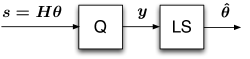
Figure 1: Signal chain of the analyzed system.

In this paper, the signal chain depicted in Fig. 1 is considered. In this Figure, $s$ represents the input sequence, $\theta$ the vector of parameters to be identified and $H$ the observation matrix, that is the matrix with known entries that linearly relates $\theta$ to the input sequence. This analysis framework is customary in the identification of models that are linear in the parameters [4]. The use of an observation matrix is a more convenient way to express dependencies between parameters and observable quantities, than using lists of time–varying equations. The specification of the element in this matrix is done on the basis of the characteristics of the identification problem to be analyzed and follows standard signal processing approaches [3]. The input sequence is subjected to quantization, so that the cascaded block performs an LS analysis on a quantized version of the input signal, to provide an estimate $\hat{\theta}$ of $\theta$. To highlight the limits of the simple approach, consider the following example, based on the signal chain depicted in Fig. 1. Assume ${H}$ as a vector containing known samples of a cosine function driven by a uniformly distributed random phase, with independent outcomes

$${H}\coloneqq[h_{0}\cdots h_{N-1}]^{T},\quad h_{i}\coloneqq\cos(\varphi_{i})$$

$$s_{i}\coloneqq\theta h_{i},\quad\varphi_{i}\in{\cal U}(0,2\pi],\qquad i=0,\ldots,N-1,$$

and consider the estimation of the constant amplitude $\theta$. By assuming a $3$–bit midtread quantizer, with input range $[-1,1]$, the quantizer output sequence $y_{i}$ becomes a nonlinear deterministic function of the input $s_{i}$. The LS–based estimator of $\theta$, which also provides the Best Linear Approximation (BLA) of the overall nonlinear system is [3]

$${\hat{\theta}}=\left({H}^{T}{H}\right)^{-1}{H}^{T}{y}=\frac{\frac{1}{N}\sum_{i=0}^{N-1}y_{i}h_{i}}{\frac{1}{N}\sum_{i=0}^{N-1}h_{i}^{2}}.$$ (1)

In calculating bias and variance of ${\hat{\theta}}$, two approaches may be taken. The first approach (simple calculation) considers the quantization error as due to a noise source of independent random variables with uniform distribution in $\left[-\frac{\Delta}{2},\frac{\Delta}{2}\right)$ with $\Delta=2/2^{b}$ as the quantization step and $b$ as the number of quantizer bits. The second approach (exact calculation) takes quantization effects into consideration and precisely allows assessment of estimator bias and variance. It will be shown next how the simple approach may lead to inaccurate results, underestimating the effects of quantization. By using the simple calculation approach, $y_{i}$ becomes

$$y_{i}=\theta h_{i}+e_{i},\qquad i=0,\ldots,N-1,$$

where $e_{i}$ represents the quantization error, considered independent from $\theta h_{i}$ and uniformly distributed in $\left[-\frac{\Delta}{2},\frac{\Delta}{2}\right)$. Under this assumption, in App. A it is shown that,

$$E(\hat{\theta})\simeq\theta,\qquad\mbox{Var}(\hat{\theta})\simeq\frac{\Delta^{2}}{6N}.$$ (2)

To verify the validity of the simplified approach, simulations have been carried out. Both the variance of ${\hat{\theta}}$ obtained by the simplified calculation and that estimated using the samples at the quantizer output are plotted in Fig. 2. In this Figure, data have been normalized to $\Delta^{2}/(6N)$ and plotted as a function of the input amplitude normalized to $\Delta$.

Figure 2: Variance of $\hat{\theta}$ normalized to the theoretical variance $\Delta^{2}/(6N)$ obtained by the simple approach ($3$–bit quantizer): Montecarlo–based estimations based on the quantizer output sequence (solid line) and on the simplified assumption about the error sequence (dotted line). Estimates obtained using a $3$–bit quantizer, $15\cdot 10^{3}$ records, each one containing $N=200$ samples.

As it is clear from Fig. 2, the simplified calculation provides a variance that underestimates the true variance by more than $100\%$ for several values of the parameter $\theta$. This is not surprising because of the strong nonlinear distortion introduced by the quantizer, but needs to be addressed. The standard deviation of ${\hat{\theta}}$ is related to the standard uncertainty in the estimation of $\theta$ [17]. This motivates the analysis of the effects of quantization, when LS–based estimators are used to infer parameter values and corresponding uncertainties. It is reasonable to assume that by increasing the quantizer resolution, this effect will vanish for large values of $\theta$. At the same time, it is expected that even in the case of high resolution quantizers this phenomenon will be relevant, especially for small values of the ratio $\theta/\Delta$.

III Least Square Based Estimator of the Square Amplitude of a Quantized sine wave

III-A Signal and System

The main estimation problem analyzed in this paper, considers an instance of the signal chain depicted in Fig. 1 based on the following assumptions:

• (Assumption 1) The quantizer input signal is a coherently sampled sine wave, defined by

  $$s_{i}\coloneqq-A\cos(k_{i}+\varphi),\quad k_{i}\coloneqq\frac{2\pi\lambda}{N}i,\quad i=0,\ldots,N-1$$ (3)

  where $\lambda$ and $N$ are co–prime integer numbers, $A>0$, $A^{2}$ and $A$ are the parameters to be estimated and $\varphi$ is the record initial phase. The coherency condition requires both synchronous sine wave sampling and observation of an integer number of sine wave periods. Since $s_{i}$ may also be affected by a deterministic offset or by random noise, subsections III-H and  III-I show the estimator performance under these additional assumptions, respectively.

• (Assumption 2) The variable $\varphi$ is a random variable, uniformly distributed in $[0,2\pi)$.

When $s_{i}$ is quantized using a mid–tread quantizer, the observed sequence becomes:

$$y_{i}\coloneqq\Delta\left\lfloor\frac{s_{i}}{\Delta}+0.5\right\rfloor=s_{i}+e_{i}(s_{i}),\qquad i=0,\ldots,N-1$$ (4)

where $e_{i}(s_{i})\coloneqq y_{i}-s_{i}$ represents the quantization error. As an example, this model applies when testing ADCs [2] or in any other situation in which the amplitude or square amplitude of a sine wave are estimated on the basis of quantized data (e.g. in the area of power quality measurements). Since this is the information usually available when using modern instrumentation, (3) applies to several situations of interest in the engineering practice.

Assumption 2 is a relevant one because, usually, the value of the initial record phase, may not be controllable or may be controllable up to a given maximum error. Therefore, when comparing estimates obtained under reproducibility conditions in different laboratories or set–up’s, the value of $\varphi$ introduces a variability in the estimates. The consequences of this variability are the main subject of this paper.

We will first consider the LS–based estimation of $A^{2}$. This choice eases the initial analysis of the estimator properties since its mathematical expression becomes the summations of weighted products of observable quantities, as shown in (7). The alternative would be to estimate directly $A$. However, the additional nonlinear effect of the square–root operation implied by extracting $A$ from $A^{2}$, further complicates the analysis and is treated in subsection III-G. According to (3), the model to be fitted, by using the observed sequence $y_{i}$, is

$$s_{i}=-A\cos(\varphi)\cos(k_{i})+A\sin(\phi)\sin(k_{i})\quad i=0,\ldots,N-1,$$

that can be rewritten in matrix form as [4]:

$$S=H\theta$$

where $S\coloneqq[s_{0}\quad s_{1}\quad\cdots\quad s_{N-1}]^{T}$,

$${\theta}\coloneqq\left[{\theta}_{1}\quad{\theta}_{2}\right]^{T}\coloneqq\left[A\cos(\varphi)\quad A\sin(\varphi)\right]^{T}$$

is the parameter vector and

$$H\coloneqq\left[\begin{array}[]{cc}-\cos(k_{0})&\sin(k_{0})\\ -\cos(k_{1})&\sin(k_{1})\\ \vdots&\vdots\\ -\cos(k_{N-1})&\sin(k_{N-1})\end{array}\right],$$

is the observation matrix. Define

$${\hat{\theta}}\coloneqq\left[{\hat{\theta}}_{1}\quad{\hat{\theta}}_{2}\right]^{T}\coloneqq\left[\widehat{A\cos(\varphi)}\quad\widehat{A\sin(\varphi)}\right]^{T}$$

as the estimator of $\theta$. Since $\theta^{2}=\theta_{1}^{2}+\theta_{2}^{2}$, a natural estimator ${\hat{A}}^{2}$ of $A^{2}$, results in [2]

$${\hat{A}}^{2}={\hat{\theta}}_{1}^{2}+{\hat{\theta}}_{2}^{2}$$ (5)

The LS–based estimator of $\theta$ is [4]:

$$\hat{\theta}=\left(H^{T}H\right)^{-1}H^{T}Y$$ (6)

where $Y\coloneqq[y_{0}\quad\cdots\quad y_{N-1}]^{T}$. By the coherence hypothesis, and by the orthogonality of the columns in $H$, when $N\geq 3$,

$$\left(H^{T}H\right)^{-1}=\frac{1}{N}\left[\begin{array}[]{cc}2&0\\ 0&2\\ \end{array}\right]$$

and (6) provides [5],

$${\hat{\theta}}_{1}=-\frac{2}{N}\sum_{i=0}^{N-1}y_{i}\cos\left(k_{i}\right),\qquad{\hat{\theta}}_{2}=\frac{2}{N}\sum_{i=0}^{N-1}y_{i}\sin\left(k_{i}\right)$$

that, apart from the signs, are equal to the coefficients of order $\lambda$, in a discrete Fourier transform of the observed sequence. Thus, from (5)

$$\hat{A}^{2}=\frac{4}{N^{2}}\sum_{i=0}^{N-1}\sum_{u=0}^{N-1}y_{i}y_{u}\cos\left(k_{i}-k_{u}\right)$$ (7)

Observe that, being a weighted combination of discrete random variables, $\hat{A}^{2}$ is a discrete random variable, whose properties are analyzed in the following assuming both the simple calculation and the direct calculation approaches.

III-B Mathematical Modeling

While the subject of quantization has extensively been addressed in the scientific literature, it always has proved to be a hard problem to tackle, because of the nonlinear behavior of the input–output quantizer characteristic. The mathematical modeling used in this paper, is based on several approaches used to cross–validate obtained results. Modeling is performed both in the amplitude– and in the frequency–domains. When the Amplitude Domain Approach (ADA) is considered, the quantizer output is modeled as the sum of indicator functions weighted by a suitable number of quantization steps $\Delta$, extending the same approach presented in [18] (App. B). When the Frequency Domain Approach (FDA) is considered, the quantization error sequence $e_{i}(\cdot)$ given by

$$e_{i}(s_{i})=\frac{\Delta}{2}-\Delta\left\langle\frac{s_{i}}{2}+\frac{1}{2}\right\rangle,\qquad i=0,\ldots,N-1$$ (8)

with $\langle\cdot\rangle$ as the fractional part operator, is expanded using Fourier series, as done, for example, in [1] (App. C and App. D). Both approaches show insights into the problem and provide closed–form expressions for the analyzed estimator parameters. Moreover, both techniques are easy to code on a computer. Thus they can be used to find quick values of error bounds, when mathematical expressions cease to offer easy interpretations of asymptotic behaviors and of order of magnitudes. A Montecarlo analysis has also been used to confirm mathematical results, indicated in the following as MA$(R)$, with $R$ being the number of assumed records. In this case, we used both C–language coded LS–based estimators exploiting the LAPACK numerical library, to achieve state-of-the-art efficiency in numerical processing and MATLAB, itself a commercial LAPACK wrapper [19].

III-C Statistical Assumptions

(Assumption 3) The main system analyzed in this paper is based on the assumption that quantization is applied to noise–free sine wave samples generated by (3). So would not it be for the random initial phase, the estimator output would perfectly be predictable, being a deterministic function of system and signal parameters. As it is known, wideband noise added before quantization acts as a dithering signal, that smooths and linearizes the quantizer nonlinear characteristics, at the price of an increased estimator’s variance [18]. Therefore, the main analysis described in this paper, provides knowledge about the estimator performance under the limiting situations in which the effects of the quantizer finite resolution are dominating over the effects of additive noise. This is of practical interest, given that applications exist dealing with the estimation of sine wave amplitudes based on very few samples, for low–complexity industrial purposes [20][21]. Consequently, the assessment of the conditions under which quantization does or does not influence estimators’ performance, is necessary to compensate for the lack of variance suppression benefits usually associated to averaging of a large number of samples. Because of the Assumption 2, the randomness in the signal is due to $\varphi$, that models the lack of information regarding synchronization between sample rate and sine wave frequency. Therefore, all expected values in the appendices are taken with respect to realizations of $\varphi$. When assumption 3 does not apply an additional source of randomness contributes to modify the estimator bias and variance properties. This corresponds to the practical situation in which, e.g. when testing ADCs, the input sine wave is corrupted by Gaussian noise. The analysis of this case is done in subsection III-I.

(a)

(b)

Figure 3: MA$(5\cdot 10^{3})$: standard deviation of ${\hat{A}^{2}}$ normalized to $A$ when $N=2\cdot 10^{3}$, $b=13$: simple approach (dashed line) and direct approach based on (7) (solid line): (a) $\lambda=201$, (b) $\lambda=200$.

III-D Synchronizations issues: Sampling and Sine Fit LS–based Estimation

As pointed out in [2][5], in practice, the synchronous condition implied by Assumption 1, can be met up to the frequency errors associated with the equipment used to provide experimental data. This is the case, for instance, when testing ADCs: an accurate sine wave generator provides the test signal to the device under test and the quantizer output data are processed to estimate the input signal parameters, needed for additional processing [2]. In this case, errors in the ratio between the ADC sampling rate and the sine wave frequency may result in major errors when estimating other related parameters [22]. When Assumption 1 is not met, also the properties of (7) change significantly. As an example, consider the two coprime integers $N=2000$ and $\lambda=201$. The normalized standard deviation of ${\hat{A}^{2}}$ obtained by the LS–based estimator is plotted in Fig. 3(a), as a function of $A$ (solid line), when $b=13$. In the same figure also the normalized estimator standard deviation is plotted, when considering the simple approach, that models quantization as due to the effect of additive uniform noise (dashed line). Standard deviations in Fig. 3 are estimated using MA$(5\cdot 10^{3})$. Fig. 3(a) shows that the simple assumption almost uniformly underestimates the standard deviation. Now assume that, due to inaccuracies in the experimental setup, the ratio $\lambda/N$ becomes the ratio of two integers with common dividers such as $200/2000=1/10$. The same results as those shown in Fig. 3(a) are plotted in Fig. 3(b). Two outcomes are evident: the additive noise model still provides the same results as those in Fig. 3(a), while that based on (7) has a much larger standard deviation, increased by $20$ times. This can be explained by observing that, because of quantization, only $10$ samples of (3) having different instantaneous phases are in the dataset. This does not modify the standard deviation in the case of the simple approach because the superimposed additive noise still provides useful information, also for those samples associated to the same instantaneous phase. On the contrary, when noise–free data are quantized, samples associated to the same instantaneous phase provide the same quantized output value for a given initial record phase $\varphi$ and the estimator uses exactly the same data points affected by strongly correlated quantization error, over different sine wave periods. In this latter case, the amount of available information is greatly reduced over the case in which no quantization is applied and we can conclude that this phenomenon is not modeled properly by the simple approach, that provides overly optimistic results. When Assumption 1 does not hold true, and the need is that of also taking into account the finite synchronization capabilities between sample rate and sine wave test frequency, an approach based on the Farey series can be adopted [22].

(a)

(b)

(c)

(d)

Figure 4: FDA and ADA: normalized bias in the estimation of $A^{2}$ evaluated by assuming $N=2\cdot 10^{3}$, $\lambda=201$, $\{4,6,8,12\}$ bit (FDA–solid line, ADA–squares) and $B_{2}(\Delta)$ (stars and dashed line).

III-E Square Amplitude LS–Based Estimation: Bias

As pointed out in [10] the LS–based estimator (7) is biased. The bias can be much larger than that predicted by the simple approach. In App. C it is shown that the bias in the estimation of the square amplitude is given by

$$\begin{split}bias(A,\Delta,N)&\coloneqq E({\hat{A}}^{2})-A^{2}=\\ &=4Ag(A,\Delta)+8h(A,\Delta,N)=\\ &\overset{N\rightarrow\infty}{=}4g(A,\Delta)\left[A+g(A,\Delta)\right]\coloneqq bias(A,\Delta)\end{split}$$ (9)

where

$$g(A,\Delta)\coloneqq\left\{-\frac{x}{2}+\frac{\sqrt{\pi}}{x\Gamma\left(\frac{3}{2}\right)}\sum_{k=1}^{p}\left[x^{2}-\left(k-\frac{1}{2}\right)^{2}\pi^{2}\right]^{\frac{1}{2}}\right\}$$ (10)

with $x\coloneqq\pi A/\Delta$, $\Gamma(\cdot)$ as the gamma function and

$$p\coloneqq\left\lfloor\frac{x}{\pi}+\frac{1}{2}\right\rfloor=\left\lfloor\frac{A}{\Delta}+\frac{1}{2}\right\rfloor$$ (11)

and (App. C),

$$h(A,\Delta,N)\coloneqq\frac{\Delta^{2}}{\pi^{2}N^{2}}\sum_{i=0}^{N-1}\sum_{u=0}^{N-1}\cos(k_{i}-k_{u})\\ \cdot\sum_{k=1}^{\infty}\sum_{h=1}^{\infty}\frac{(-1)^{h+k}}{hk}\sum_{n=0}^{\infty}J_{2n+1}(z_{h})J_{2n+1}(z_{k})\\ \cdot\cos((2n+1)(k_{i}-k_{u}))$$ (12)

Expressions $g(A,\Delta)$ and $bias(A,\Delta,N)$ do not uniformly vanish with respect to $A$, for any finite value of $\Delta$, even when $N\rightarrow\infty$. Thus, (7) is a biased and inconsistent estimator of $A^{2}$. Simulations show that few hundreds samples are sufficient for the bias to achieve convergence to $bias(A,\Delta)$ when $b<20$. Two bounds on $|bias(A,\Delta)|$ are derived in App. E. The first one, $B_{1}(A,\Delta)$, is based on a bound on Bessel functions and is given by:

$$B_{1}(A,\Delta)\coloneqq 4AB(A,\Delta)+4B(A,\Delta)^{2}$$ (13)

where

$$B(A,\Delta)\coloneqq\Delta^{\frac{4}{3}}\frac{\zeta\left(\frac{4}{3}\right)c}{\pi\left(2\pi A\right)^{\frac{1}{3}}},$$ (14)

where $\zeta(s)=\sum_{k=1}^{\infty}\frac{1}{k^{s}}$ is the Riemann zeta function and $c=0.7857\ldots$. The second one, $B_{2}(\Delta)$, is based on a finite sum expression of $g(A,\Delta)$ and is given by (see E.4):

$$B_{2}(\Delta)=4Ag\left(\left(p-\frac{1}{2}\right)\Delta,\Delta\right)\quad p=0,1,\ldots$$ (15)

While $B_{1}(A,\Delta)$ is a (somewhat loose) upper bound on $|bias(A,\Delta)|$ for given values of $A$ and $\Delta$, $|B_{2}(\Delta)|$ is a tighter bound, obtained with some approximations, that provides the discrete envelope of the minima in $bias(A,\Delta)$ (App. E). The expression for $B_{1}(A,\Delta)$ shows that the absolute value of the bias in the estimation of $A^{2}$ is on the order of $O\left(\Delta^{\frac{4}{3}}\right)$, when $\Delta\rightarrow 0$.

To illustrate the behavior of derived expressions, $bias(A,\Delta)$ is plotted in Fig. 4, when assuming $b=4,6,8,12$ bit and $N=2\cdot 10^{3}$. Plots, calculated using FDA and ADA (solid lines and square symbols, respectively) have been normalized to $\Delta^{4/3}$ to validate the assumption on the approximate rate of convergence of the bias with respect to $\Delta$. The approximate equality of the range of values in Fig. 4, irrespective of the number of bits, supports this statement. In Fig. 4, $B_{2}(\Delta)$ is plotted using stars joined by a dashed line. Direct inspection of Fig. 4 shows that the absolute values of the minima are larger than those of the maxima. Therefore it is conjectured that the curve obtained through $|B_{2}(\Delta)|$ is an approximate and tight upper bound on $|bias(A,\Delta)|$. This hypothesis is confirmed by simulation results based on a MA$(5\cdot 10^{3})$ and shown in Fig. 6. Data are obtained by assuming $N=2\cdot 10^{3}$ and $\lambda=539$. The maximum magnitude of the bias has been estimated over $0\leq A<1-\frac{\Delta}{2}$, when $b=1,\ldots,19$. The dashed line represents $|B_{2}(\Delta)|$ and circles are obtained by estimating the maximum of $|bias(A,\Delta)|$ as a function of the number of bits. The maximum of $A$ has been limited to $1-\Delta/2$, so to limit the analysis to granular quantization error, when considering quantizers with limited no–overload range, as it happens in practical usage of ADCs. The corresponding points obtained by assuming the simple approach are plotted using stars, while the continuous line represents the minimum value of the upper bound $B_{1}(\frac{1}{2},\Delta)$ (App. E). The plot shows the very good agreement between $|B_{2}(\Delta)|$, derived through the FDA, and maxima obtained using the MA$(5\cdot 10^{3})$.

The difference in slopes between $B_{1}(\frac{1}{2},\Delta)$ and $|B_{2}(\Delta)|$ explains the reduction in the range values in Fig. 3, as the number of bits increases. Consequently, it is conjectured that the absolute value of the bias vanishes faster the $\Delta^{\frac{4}{3}}$ when $\Delta\rightarrow\infty$, which is consistent with the large amplitude approximation of the Bessel functions, for large values of their argument [23]. Fig. 6 shows also clearly that the simple approach strongly underestimates the maxima. The asymptotic behavior of $bias(A,\Delta,N)$ for large values of $N$ is shown in Fig. 6, where results based on both the MA$(10^{6}\div 5\cdot 10^{3})$ and the ADA are shown for a $10$ bit quantizer, when $A=10.93\Delta$. Clearly, the convergence rate is quick, as when $N>100$, already the asymptotic value is achieved. A variable number of records has been used because convergence of Montecarlo–based algorithms depends on $N$: when $N$ is small a much larger number of records is needed than when $N$ is large.

Figure 5: MA$(2\cdot 10^{3})$ and FDA; normalized maximum in the bias of the square amplitude estimator over all possible values of the input amplitude $0\leq A\leq 1-\Delta/2$ (circles) and based on the simple approach (stars). Shown are also the upper bound $B_{1}(\frac{1}{2},\Delta)$ (solid line) and the approximate upper bound $|B_{2}(\Delta)|$ (dashed line).

Figure 6: MA$(10^{6}\div 5\cdot 10^{3})$ and ADA; main figure: normalized bias in the estimation of $A^{2}$, as a function of $N=3,\ldots,300$, when assuming $b=10$ bit and $A=10.93\Delta$. For large values of $N$, the graph converges to $0.9398\ldots$, as predicted by (E.1). In the inset, the difference between the Montecarlo–based estimator and the theoretical expression $bias(A,\Delta,N)$ derived from (C.19) and normalized to $\Delta^{2}$.

Figure 7: MA$(5\cdot 10^{3})$, $N=2\cdot 10^{3}$. Normalized maximum in the variance of the square amplitude estimator over all possible values of the input amplitude $0\leq A\leq 1-\Delta/2$ (dashed line) and based on the simple approach (dots). Shown is also the theoretical variance derived in [5][9] under the assumption of zero–mean additive Gaussian noise with variance $\Delta^{2}/12$ (solid line).

Figure 8: MA$(5\cdot 10^{3})$ , $N=2\cdot 10^{3}$. Normalized maximum of the mean square error over all possible values of the input amplitude $0\leq A\leq 1-\Delta/2$ (solid line). Shown is also the normalized maximum square bias (solid–dotted line) and variance (dashed line).

III-F Square Amplitude LS–Based Estimation: Variance and Mean Square Error

The variance of (7) can again be calculated using the modeling techniques listed in Sect. III-B and applied as in App. B and App. D. To highlight the risks associated to the usage of the simple approach to calculate uncertainties in the estimation of the square amplitude, consider the graphs shown in Fig. 8. Data in this figure have been obtained using MA$(5\cdot 10^{3})$ under the same conditions used to generate data in Fig. 6 and represent the normalized maximum in the variance, over $0<A\leq 1-\frac{\Delta}{2}$: the dashed line has been obtained when using quantized data. Dots represent the behavior of the maximum in the estimator variance when the simple model is assumed. The solid line represents its value published in [5][9], obtained by neglecting quantization and by assuming zero–mean additive Gaussian noise, having variance $\Delta^{2}/12$. Clearly, the simple model underestimates the variance, even when the number of bit is large. The increasing behavior of the dashed line is due to the large estimator bias associated with low values of $b$. When $b$ increases, the bias uniformly vanishes and the variance increases accordingly. This is a trend similar to that described in [9], to explain the super–efficiency in the behavior of the LS–based estimator under the hypothesis of zero–mean additive Gaussian noise. This behavior is better seen in Fig. 8 where the normalized Mean Square Error (MSE) is plotted together with the the normalized square bias and variance, maximized over all possible values of $0<A\leq 1-\frac{\Delta}{2}$, as a function of the number of bits. Data in Fig. 8 are obtained by the MA$(5\cdot 10^{3})$ and considering $N=2\cdot 10^{3}$ sine wave samples, with $\lambda=539$. The crossing between curves explains more clearly the super–efficiency type of effect shown in Fig. 8.

In App. D, it is proved that the variance vanishes when $N\rightarrow\infty$. From a practical viewpoint, the speed of convergence is quick, as shown in Fig. 9, where the MA$(5\cdot 10^{3}\div 10^{6})$ has been applied to evaluate the estimator variance, assuming $b=10$ bit and $A=10.93\Delta$. A variable number of records has been used in the Montecarlo method, to keep the simulation time approximately constant for each value of $N$, as $N$ increases. In fact, when $N$ is small, a larger number of records is needed to reduce estimators’ variance, than for larger values of $N$.

Figure 9: MA$(5\cdot 10^{3}\div 10^{6})$ and ADA; main figure: normalized estimator variance as a function of $N$, when $b=10$ and $A=10.93\Delta$. Inset: difference between expressions derived using the MA$(5\cdot 10^{3})$ and the ADA, normalized to $\Delta^{4}$.

III-G Amplitude LS–Based Estimation: Bias

Results described in section III-B–III-F allow calculation of the mean value of the LS–based estimator ${\hat{A}}\coloneqq\sqrt{\hat{A}^{2}}$ of the amplitude $A$ in (7). While, it is well known that nonlinear transformations such as the extraction of the square–root, do not commute over the expectation when calculating the moments of a random variable, by using a Taylor series expansion about the mean value of ${\hat{A}^{2}}$, we have [4]:

$$E\left({\hat{A}}\right)\simeq\sqrt{E\left({\hat{A}^{2}}\right)}-\frac{\mbox{Var}({\hat{A}^{2}})}{8\sqrt{\left[E\left({\hat{A}^{2}}\right)\right]^{3}}},\qquad\mbox{Var}({\hat{A}^{2}})\rightarrow 0$$ (16)

When $N\rightarrow\infty$ the variance of the square estimator vanishes as proved in sec. III-F. Therefore, we have $E\left({\hat{A}}\right)\overset{N\rightarrow\infty}{\simeq}\sqrt{E\left({\hat{A}^{2}}\right)}.$ To illustrate the validity of this approximation, results are shown in Fig. 10, in which the normalized bias in the LS–based estimation of the sine wave amplitude is plotted. The main figure shows the behavior of the bias, obtained by using the MA$(5\cdot 10^{3})$, when $N=500$, $\lambda=137$ and $b=8$. In the same figure, the inset shows the difference in bias estimation when using (16) and the MA($5\cdot 10^{3}$). Since the Montecarlo approach does not rely on the approximations induced by the Taylor series expansion, it proves the validity of this estimation method. Consequently, all properties of the square amplitude estimator such as the inconsistency, and the behavior of the bias and of its maxima, can easily be adapted by taking the square root of the estimators analyzed in sec. III-B–III-F, in the limit $N\rightarrow\infty$.

Figure 10: MA$(5\cdot 10^{3})$ and ADA; main figure: normalized estimator bias as a function of $A/\Delta$, when $b=10$. Inset: difference between expressions derived using the MA$(5\cdot 10^{3})$ and the ADA, normalized to $\Delta$.

(a)

(b)

Figure 11: ADA: normalized bias in the estimation of $A^{2}$ evaluated by assuming $N=2\cdot 10^{3}$, $\lambda=201$, $\{4,6\}$ bit assuming an input sine wave offset taking values in $\{-\nicefrac{{\Delta}}{{2}},-\nicefrac{{\Delta}}{{2}}+\nicefrac{{\Delta}}{{10}},-\nicefrac{{\Delta}}{{2}}+\nicefrac{{2\Delta}}{{10}},\ldots,\nicefrac{{\Delta}}{{2}}\}$. Shown is also the arithmetic mean of the bias curves and $B_{2}(\Delta)$ (stars and dashed line).

III-H Squared Amplitude LS–Based Estimation Bias: Effect of Input Offset

The models described in this paper allow the analysis of the estimator performance also when the input signal has a non–zero mean value, that is when (3) is modified to include an additive constant $d$ as follows:

$$s_{i}\coloneqq-A\cos(k_{i}+\varphi)+d,\quad k_{i}=\frac{2\pi\lambda}{N}i,\quad i=0,\ldots,N-1.$$

As an example, this case is relevant when the sine wave is used as a test signal for assessing ADC performance. Precisely controlling the mean value up to the accuracy required by the quantization step width, may not be an easy task, especially for small ADC resolutions. At the same time, temperature and voltage drifts may induce variations in input–related offset voltages in the considered ADC. Therefore, bounds on the estimation error need to include also the effect of $d$. Including an offset in the input signal may be equivalent to modeling a quantizer other than the mid–tread one considered in (4), acting on an offset–free sine wave. As an example, if $d=-\left(\nicefrac{{\Delta}}{{2}}\right)$, (4) becomes the model of a truncation quantizer applied to (3). To verify the implications of an additive constant in the input signal, the bias in estimating $A^{2}$ has been evaluated using the $ADA$, under the same conditions used to generate data shown in Fig. 4. In Fig. 11(a)–(b), corresponding to Fig. 4(a)–(b), is shown the normalized bias, when assuming $b=4,6$. In this Figure, $d$ is assumed as a parameter taking values in $-\left(\nicefrac{{\Delta}}{{2}}\right),\ldots,\nicefrac{{\Delta}}{{2}}$ in steps of $\nicefrac{{\Delta}}{{10}}$. The overall behavior shows that the added offset does not worsen the bias with respect to data shown in Fig. 4. The bold line in Fig. 11 is the arithmetic mean of all curves. Thus, it approximates the behavior of the bias when $d$ is taken as being a random variable uniform in $\left[-\frac{\Delta}{2},\frac{\Delta}{2}\right)$.

Figure 12: MA$(2\cdot 10^{3})$: normalized maximum in the bias of the square amplitude estimator over all possible values of the input amplitude $0\leq A\leq 1-\Delta/2$ (circles), by assuming zero–mean additive Gaussian noise having the indicated standard deviation. Shown is also the normalized maximum obtained by the simple approach (stars), the upper bound $B_{1}(\frac{1}{2},\Delta)$ (solid line) and the approximate upper bound $|B_{2}(\Delta)|$ (dashed line).

Figure 13: MA$(5\cdot 10^{3})$, $N=2\cdot 10^{3}$. Normalized maximum in the variance of the square amplitude estimator over all possible values of the input amplitude $0\leq A\leq 1-\Delta/2$ (circles and solid line), by assuming zero–mean additive Gaussian noise having the indicated standard deviation. Shown is also the normalized maximum obtained by the simple approach (stars) and the theoretical variance derived in [5][9] under the assumption of zero–mean additive Gaussian noise with variance $\Delta^{2}/12$ (dashed lines).

III-I Squared Amplitude LS–Based Estimation Bias: Effect of Input Noise

The quantizer input sine wave may be affected by additive wide–band noise $n_{G}$, as follows:

$$s_{i}\coloneqq-A\cos(k_{i}+\varphi)+n_{G},\quad k_{i}=\frac{2\pi\lambda}{N}i,\quad i=0,\ldots,N-1.$$

As it is well–known, noise act as a dither signals (unsubtractive dither in this case) and under suitable conditions, it renders the quantization error a uniformly distributed random variable, regardless of the input signal distribution [1, 16]. The overall effect of properly behaving input–referred additive noise is that of linearizing the mean value of the quantizer input–output characteristic. Consequently, a reduction in the estimation bias shown in Fig. 4 and Fig. 11 is expected. This will come at the price of an increased estimation variance. In fact, an additional source of uncertainty characterizes the estimator input data, beyond that taking into account the initial record phase. Additive zero–mean Gaussian noise has been considered in the following, having standard deviation $\sigma_{n}\in\{0,\nicefrac{{\Delta}}{{5}},\nicefrac{{2\Delta}}{{5}},\nicefrac{{3\Delta}}{{5}}\}$. To verify the implications of additive Gaussian noise, the bias in estimating $A^{2}$ has been evaluated using the $MA(2\cdot 10^{3})$, under the same conditions used to generate data shown in Fig. 6 and Fig. 8. Results are plotted in Fig. 13 and Fig. 13, respectively. Plots in Fig. 13 show that by increasing the noise standard deviation the bias decreases and tends toward the value associated to the use of the noise model of quantization (graphed using stars). Even though Gaussian noise does not have the properties necessary to make the quantization error become a uniform random variable, it approximates such behavior as its variance increases. Results are also consistent with data in [8], where it is shown that for values of $\sigma/\Delta>0.3$, the overall quantization error tends to Gaussianity regardless of the ADC resolution. At the same time Fig. 13 shows that the normalized maximum value of the estimation variance increases with the noise variance, as expected, irrespective of the quantizer resolution.

IV Results and Discussion

It is high–priority of the instrumentation and measurement community to understand error bounds when using procedures and algorithms to analyze data. Thus, the results in this paper serve a double role: warn against the usage of the noise model of quantization to provide bounds on estimation errors when using the LS–algorithm on quantized data and show how to include the effect of quantization when doing calculations needed to derive such bounds.

IV-A Some Application Examples

Results have practical relevance. As an example, consider the case when two different laboratories want to compare results obtained when measuring electrical parameters of the same ADC. Research on these devices is ongoing and produces design and realizations optimizing various criteria, most generally including resolution, speed of conversion and energy consumption. Low resolution ADCs are used in ultra–wide bandwidth receivers (5 bits) [11], serial links (4.5 bits) [12], hard–disk drive read channels (6 bit) [13] and waveform capture instruments and oscilloscopes (8 bit) [14]. Conversely low–conversion rate, high resolution ADCs are employed, for instance, in industrial instrumentation or in digital audio applications. Regardless of the device resolution, all ADCs undergo testing procedures, that must be accurate, fast and sound from a metrological point of view. The majority of standardized tests require sine waves as stimulating signals [2], whose parameters (e.g. amplitude) are obtained by using LS–based estimators applied to the quantized data sequence provided by the device–under–test [7]. Synchronizing the initial record phase of the sinusoidal signal, can be done only at the expense of added instrumental complexity and up to a certain uncertainty. Therefore, allowing it to freely varying among collected data records, as it is done frequently in practice, implies an added source of variability in the results, that can be modeled by assuming a random initial record phase. The sine wave amplitude is the input parameter for the estimation of many relevant ADC parameters, such as the number of effective bits. Thus, the performed analysis shows what to expect in the amplitude estimator properties, when the initial record phase can not be controlled over different realizations of the same ADC testing procedure, under repeatability conditions. The same also applies, when two laboratories verify the level of compatibility in the estimates of the sine wave amplitude, under reproducibility conditions: the uncertainty associated to the phase variability must be taken into account. While simulations may provide directions for further investigations and hints on the existence of unexpected phenomena, they must be accompanied by analyses made to reduce the role of subjective interpretations. Mathematically–derived bounds presented in this paper serve this scope. As an example, consider the case in which the normalized difference in the sine wave amplitude estimated by the two laboratories or over different realizations of the same ADC testing procedure is larger than what can be predicted by data shown in Fig. 10, applicable as an example to a 10 bit resolution ADC. Then, variability in the initial record phase can not be the unique cause and sources of uncertainty other than those associated to the effects of quantization must be looked for.

As an additional usage example consider a medium–resolution (e.g. 10 bit) ADC embedded in a microcontroller. The acquisition and estimation of the amplitude of a sine wave is a typical problem in many engineering areas. This happens for instance when measuring power quality, when performing built–in–self–test procedures to assess functional status of system–level devices or when taking impedance measurements using sine–fitting techniques [15]. Simple sinusoidal sources used frequently in this latter case, may not allow synchronized acquisition, while synchronization with the phase of the power network in the former case, may not be feasible at reasonable costs or uncertainty levels. In both cases, LS–based estimation of the amplitude of the sinusoid is done at signal processing level and requires assessment of the associated uncertainties. Results in Fig. 5 and 6 can be used to this aim in accordance with procedure written in [17], while corresponding expressions in the appendix can be used to cope with different quantizers’ resolutions and records lengths.

IV-B Influence of Input Signal Properties

Situations occur in which tests are performed on a reduced number of output codes, that is only few among all possible ADC codes are excited. Similarly, systems such as those in Fig.1 may be sourced by sine waves with arbitrary large or small amplitudes within the admitted input range. When this case, even high–resolution ADCs may induce large relative errors in amplitude estimates, as those associated to low–resolution ADCs. As an example, consider a $16$ bit ADC used in Fig. 1 to quantize a a sine wave, whose amplitude only fully excites $256$ output codes. Fig. 4 shows that the expected behavior of the LS–based estimator is approximately that associated to an $8$ bit ADC used at full–scale, once errors have been normalized with respect to the width of the quantization step.

As shown in subsection III-I, the addition of Gaussian noise randomizes the error due to the non–linear behavior of the quantizer and reduces the estimation bias. Zero–mean uniformly distributed noise would have a similar or better linearizing behavior. With a properly set variance, uniform noise nulls the quantization error mean, while making the quantization error variance, input–signal dependent (noise modulation.). As data in Fig. 13 show, also an input offset may reduce the bias, if it randomly varies in a small–amplitude range. In this Figure, the arithmetic mean value provides almost everywhere a much smaller estimator bias with respect to any of the possible values of the offset, taken as a fixed deterministic value. The arithmetic mean is generally a reasonable estimator of the mean value of a random variable. Thus, its behavior in Fig. 13, approximates the behavior of the bias, where the input offset a random and not a deterministic value. In this case, the offset would behave as a dither signal itself.

Finally, in some applications, sequential least squares are used to provide amplitude estimations over time, when sampling an on–going continuous–time sinusoidal waveform [4]. Clearly, results presented here are applicable also in this case.

V Conclusions

In this paper, we considered LS–based estimation of the square amplitude and amplitude of a quantized sine wave. The main paper contribution is summarized by results in Tab. I. Using several analytical techniques we proved that the simple noise model of quantization provides erroneous results under several conditions and may fail, when assessing the span of estimation errors. This is especially relevant when measurement results are used for conformance testing, to assess whether manufactured products meet specified standards. As an example, ADC testing requires measurement of several parameters (e.g. ENOB) based on the estimation of the properties of testing signals such as sine waves. As shown in this paper, estimates may be affected by relevant biases that may induce in wrong decisions about the device having characteristics being under or over given thresholds. It has also been proved that the estimator is inconsistent, biased and that its variance is not predicted well by the noise model of quantization. Exact expressions have been provided that allow a rigorous evaluation of estimator properties. Both the obtained results and the methods used in this paper, are applicable also when other sine wave parameters are estimated on the basis of quantized data and when solving similar estimation problems.

Appendix A Derivation of (2)

Define

$$R\coloneqq\frac{1}{N}\sum_{i=0}^{N-1}y_{i}h_{i},\qquad S\coloneqq\frac{1}{N}\sum_{i=0}^{N-1}h_{i}^{2}$$

By using the hypothesis of zero–mean and uncorrelated random variables,

$$E(R)=E\left(\frac{1}{N}\sum_{i=0}^{N-1}(\theta h_{i}^{2}+e_{i}h_{i})\right)=\frac{\theta}{N}\sum_{i=0}^{N-1}E(h_{i}^{2})=\frac{\theta}{2}$$ (A.1)

$$E(S)=E\left(\frac{1}{N}\sum_{i=0}^{N-1}h_{i}^{2}\right)=\frac{1}{2}$$ (A.2)

Also

$$E(R^{2}) =\frac{1}{N^{2}}\sum_{i=0}^{N-1}E(y_{i}^{2}h_{i}^{2})+\frac{N(N-1)}{N^{2}}\mbox{Corr}(y_{l}h_{l},y_{k}h_{k})=$$

$$=\frac{\theta^{2}}{8N}+\frac{\Delta^{2}}{24N}+\frac{\theta^{2}}{4},\quad l\neq k$$ (A.3)

and

$$E(S^{2}) =\frac{1}{N^{2}}\sum_{i=0}^{N-1}E(h_{i}^{4})+\frac{N(N-1)}{N^{2}}\mbox{Corr}(h^{2}_{l},h^{2}_{k})=$$

$$=\frac{1}{8N}+\frac{1}{4},\quad l\neq k.$$ (A.4)

Therefore

$$\begin{split}\mbox{Var}(R)=\frac{\theta^{2}}{8N}+\frac{\Delta^{2}}{24N},\qquad\mbox{Var}(S)=\frac{1}{8N}\end{split}$$ (A.5)

and the covariance between $R$ and $S$ is given by

$$\mbox{Cov}(R,S) =\frac{1}{N^{2}}E\left(\sum_{i=0}^{N-1}(\theta h_{i}^{2}+e_{i}h_{i})\sum_{u=0}^{N-1}h_{u}^{2}\right)-\frac{\theta}{4}=$$

$$=\theta E(S^{2})-\frac{\theta}{4}=\frac{\theta}{8N}$$ (A.6)

The expected value $E(\cdot)$ and variance $\mbox{Var}(\cdot)$ of the ratio $R/S$ of two random variables, can be approximated by using a Taylor series expansion as follows [24]:

$$E\left(\frac{R}{S}\right)\simeq\frac{E(R)}{E(S)}\left\{1-\frac{\mbox{Cov}(R,S)}{E(R)E(S)}+\frac{\mbox{Var}(S)}{E^{2}(S)}\right\},$$

$$\mbox{Var}\left(\frac{R}{S}\right)\simeq\frac{E^{2}(R)}{E^{2}(S)}\left\{\frac{\mbox{Var(R)}}{E^{2}(R)}-2\frac{\mbox{Cov}(R,S)}{E(R)E(S)}+\frac{\mbox{Var}(S)}{E^{2}(S)}\right\}$$ (A.7)

Thus, by substituting (A.2)–(A.6) in (A.7), (2) follows.

Appendix B Amplitude Domain Approach: Moments of the Square Amplitude Estimator

Lemma B.1.

Assume $0\leq c<1$, $0\leq\varphi\leq 1$ and $0\leq L_{1}\leq L_{2}\leq 1$. Then, the solutions for $\varphi$, of the inequality

$$L_{1}\leq\langle c+\varphi\rangle<L_{2}$$

are

$$\begin{array}[]{ll}\{L_{1}-c\leq\varphi<L_{2}-c\}&c\leq L_{1}\\ \{0\leq\varphi<L_{2}-c\}\cup\{1-c+L_{1}\leq\varphi\leq 1\}&L_{1}<c\leq L_{2}\\ \{1-c+L_{1}\leq\varphi<1-c+L_{2}\}&c>L_{2}\end{array}$$

The proof is straightforward once observed that the expression $\langle c+\varphi\rangle$ as a function of $\varphi$, is piecewise linear:

$$\langle c+\varphi\rangle=\left\{\begin{array}[]{ll}\varphi+c&0\leq\varphi<1-c\\ \varphi-(1-c)&1-c\leq\varphi<1\end{array}\right.$$

B-A A Model for the Quantizer Output

The model described in this Appendix is based on a similar approach taken in [18]. However, it extends it in several ways: it presents a more strict mathematical formalization of the quantizer output, it includes a mathematical description of the quantizer higher–order statistical moments and it proves its applicability to the analysis of mean value and correlation of quantized stochastic processes. Assume

$$\overline{x}_{u}(\varphi)\coloneqq-\frac{A}{\Delta}\cos(k_{u}+\varphi)+0.5{+c},\qquad u=0,\ldots,N-1$$

with $A$, $\Delta$ and $c$ real numbers, $k_{u}$ a sequence of real numbers, $N$ a positive integer and $0\leq\varphi\leq 2\pi$. The constant $c$ models both the contribution of an offset in the sinusoidal signal and of an eventual offset in the quantizer input–output characteristic, as they are indistinguishable. In fact, while in this paper, mid–tread quantization is considered, by setting properly the value of $c$, other types of quantization are covered by this analysis. For instance, when $c=-0.5$, a truncation quantizer is modeled. Conversely by setting $c=\frac{d}{\Delta}$, the following analysis also comprehends the case when the input sine wave has an offset $d$. Define the quantizer output as

$$y_{u}\coloneqq\Delta\lfloor\overline{x}_{u}\rfloor,\qquad u=0,\ldots,N-1.$$

Then,

$$y_{u}=n\Delta,\qquad n\in(-\infty,\infty),\qquad n\quad\mbox{integer}{,}$$

if $\overline{x}_{u}(\varphi)$ belongs to the interval:

$$S_{n}\coloneqq\left[D_{n},U_{n}\right),$$

where $D_{n}\coloneqq\max(\min_{\varphi}\{\overline{x}_{u}(\varphi)\},n)$ and $U_{n}\coloneqq\min(\max_{\varphi}\{\overline{x}_{u}(\varphi)\},n+1)$, Consequently,

$$y_{u}=\sum_{n=-\infty}^{\infty}n\Delta i\left(\overline{x}_{u}(\varphi)\in S_{n}\right),\qquad S_{n}\coloneqq[D_{n},U_{n})$$

where $i(\cdot)$ is the indicator function of the event at its argument. For a given value of $k_{u}$, $\overline{x}_{u}(\varphi)$ will or will not belong to $S_{n}$ depending on the value of $\varphi$. In the following, it will be shown how to find the set of values that make $y_{u}=n\Delta$. This occurs when

$$D_{n}\leq-\frac{A}{\Delta}\cos\left(k_{u}+\varphi\right)+0.5{+c}<U_{n}$$ (B.1)

that is

$$\frac{\Delta}{A}\left(D_{n}-0.5{-c}\right)\leq-\cos\left(k_{u}+\varphi\right)<\frac{\Delta}{A}\left(U_{n}-0.5{-c}\right)$$

Since the cosine function is periodic with period $2\pi$, we may write:

$$\frac{\Delta}{A}\left(D_{n}-0.5{-c}\right) \leq-\cos\left(\left\langle\frac{k_{i}+\varphi}{2\pi}\right\rangle 2\pi\right)<$$

$$<\frac{\Delta}{A}\left(U_{n}-0.5{-c}\right)$$

Thus,

$$\begin{split}-\frac{\Delta}{A}\left(U_{n}-0.5{-c}\right)&<\cos\left(\left\langle\frac{k_{u}+\varphi}{2\pi}\right\rangle 2\pi\right)\leq\\ &\leq-\frac{\Delta}{A}\left(D_{n}-0.5{-c}\right)\end{split}$$ (B.2)

Define

$$L_{n}\coloneqq-\frac{\Delta}{A}\left(D_{n}-0.5{-c}\right),\qquad R_{n}\coloneqq-\frac{\Delta}{A}\left(U_{n}-0.5{-c}\right),$$

and observe that the $\arccos(\cdot)$ function is a decreasing function of its argument and returns values in $[0,\pi]$, so that by applying it to all members in (B.2) we obtain:

$$\left\{\frac{1}{2\pi}\arccos(L_{n})\leq\left\langle\frac{k_{u}+\varphi}{2\pi}\right\rangle<\frac{1}{2\pi}\arccos(R_{n})\right\}\cup$$

$$\cup\left\{\left(1-\frac{1}{2\pi}\arccos(R_{n})\right)<\left\langle\frac{k_{u}+\varphi}{2\pi}\right\rangle\leq\right.$$

$$\left.\quad\leq\left(1-\frac{1}{2\pi}\arccos(L_{n})\right)\right\}$$

Moreover, since $\left\langle a+b\right\rangle=\left\langle\langle a\rangle+\langle b\rangle\right\rangle$ and $0\leq\varphi<2\pi$, for $u=0,\ldots,N-1$, we have

$$\left\{\frac{1}{2\pi}\arccos(L_{n})\leq\left\langle\left\langle\frac{k_{u}}{2\pi}\right\rangle+\frac{\varphi}{2\pi}\right\rangle<\frac{1}{2\pi}\arccos(R_{n})\right\}\cup$$

$$\cup\left\{1-\frac{1}{2\pi}\arccos(R_{n})<\left\langle\left\langle\frac{k_{u}}{2\pi}\right\rangle+\frac{\varphi}{2\pi}\right\rangle\leq\right.$$

$$\left.\quad\leq 1-\frac{1}{2\pi}\arccos(L_{n})\right\}$$ (B.3)

Let us define $\Phi_{n}(k_{u})$, for a given value of $k_{u}$, as the sets of values of $\varphi$ such that (B.2) is satisfied. This set is to be found by applying twice the results in lemma (B.1) to the two intervals $I_{1},I_{2}$, implicitly defined in (B.3)

$$I_{1}\coloneqq\left[\frac{1}{2\pi}\arccos(L_{n}),\frac{1}{2\pi}\arccos(R_{n})\right)$$

$$I_{2}\coloneqq\left(1-\frac{1}{2\pi}\arccos(R_{n}),1-\frac{1}{2\pi}\arccos(L_{n})\right]$$

with $c=\left\langle\frac{k_{u}}{2\pi}\right\rangle$, $u=0,\ldots,N-1$. Thus,

$$y_{u}=\sum_{n=-\infty}^{\infty}n\Delta i\left(\varphi\in\Phi_{n}(k_{u})\right)$$

The set of $\Phi_{n}(k_{u})$, $n=-\infty\ldots\infty$, for any given $k_{u}$, forms a partition of the interval $[0,2\pi)$.

Figure 14: Usage example of the amplitude–domain model to calculate the correlation between two quantizer outputs ($b=3$), when $\varphi/(2\pi)$ is uniform in $[0,1)$ and $A=1$ and $c=0$: the normalized products of the two outputs (center line), must be multiplied with the width of the corresponding segment on the center line, that represents the probability of occurrence, until all contributions are summed.

Consider the product $y_{u_{1}}y_{u_{2}}\cdots y_{u_{M}}$, with integers $u_{\cdot}$ all taking values in $\{0\ldots N-1\}$. Then

$$y_{u_{1}}y_{u_{2}}\cdots y_{u_{M}}=\sum_{n=-\infty}^{\infty}n\Delta i\left(\overline{x}_{u_{1}}(\varphi)\in S_{n}\right)\cdot$$

$$\cdot\sum_{m=-\infty}^{\infty}m\Delta i\left(\overline{x}_{u_{2}}(\varphi)\in S_{m}\right)\cdots\sum_{h=-\infty}^{\infty}h\Delta i\left(\overline{x}_{u_{M}}(\varphi)\in S_{h}\right).$$

Since the intervals $S_{n}$ and $S_{m}$ have void intersection, if $m\neq n$, we can write

$$y_{u_{1}}y_{u_{2}}\cdots y_{u_{M}}=\Delta^{M}\sum_{n=-\infty}^{\infty}n^{M}i\left(\overline{x}_{u_{1}}(\varphi)\in S_{n}\right)\\ \cdot i\left(\overline{x}_{u_{2}}(\varphi)\in S_{n}\right)\cdots i\left(\overline{x}_{u_{M}}(\varphi)\in S_{n}\right)$$

that is,

$$y_{u_{1}}y_{u_{2}}\cdots y_{u_{M}}=\Delta^{M}\sum_{n=-\infty}^{\infty}n^{M}i\left(\varphi\in\Phi_{n}(k_{u_{1}})\right)\\ \cdot i\left(\varphi\in\Phi_{n}(k_{u_{2}})\right)\cdots i\left(\varphi\in\Phi_{n}(k_{u_{M}})\right)$$

Given that the indicator function can only output $0$ or $1$, by the same reasoning, we have:

$$y^{m1}_{u_{1}}y^{m2}_{u_{2}}\cdots y^{m_{M}}_{u_{M}}=\Delta^{m_{1}+m_{2}+\cdots+m_{M}}\\ \cdot\sum_{n=-\infty}^{\infty}n^{m_{1}+m_{2}+\cdots+m_{M}}i\left(\varphi\in\Phi_{n}(k_{u_{1}})\right)\\ \cdot i\left(\varphi\in\Phi_{n}(k_{u_{2}})\right)\cdots i\left(\varphi\in\Phi_{n}(k_{u_{M}})\right)$$ (B.4)

where $m_{1},m_{2},\cdots,m_{M}$ are integer values. Thus, the product

$$y^{m_{1}}_{u_{1}}y^{m2}_{u_{2}}\cdots y^{m_{M}}_{u_{M}}$$

is a deterministic function of $\varphi$. If $\varphi$ becomes a random variable distributed in $[0,2\pi)$, then (B.4) allows the calculation of joint moments of the quantizer output as follows

$$E\left(y^{m_{1}}_{u_{1}}y^{m2}_{u_{2}}\cdots y^{m_{M}}_{u_{M}}\right)=\Delta^{m_{1}+m_{2}+\cdots+m_{M}}\\ \cdot\sum_{n=-\infty}^{\infty}n^{m_{1}+m_{2}+\cdots+m_{M}}\cdot E\left(i\left(\varphi\in\Phi_{n}(k_{u_{1}})\right)\right.\\ \cdot\left.i\left(\varphi\in\Phi_{n}(k_{u_{2}})\right)\cdots i\left(\varphi\in\Phi_{n}(k_{u_{M}})\right)\right)$$

The argument of the expectation in the summation is a Bernoulli random variable. Therefore,

$$E\left(y^{m_{1}}_{u_{1}}y^{m2}_{u_{2}}\cdots y^{m_{M}}_{u_{M}}\right)=\Delta^{m_{1}+m_{2}+\cdots+m_{M}}\\ \cdot\sum_{n=-\infty}^{\infty}n^{m_{1}+m_{2}+\cdots+m_{M}}\cdot\mbox{Pr}\left(i\left(\varphi\in\Phi_{n}(k_{u_{1}})\right)\right.\\ \left.\cdot i\left(\varphi\in\Phi_{n}(k_{u_{2}})\right)\cdots i\left(\varphi\in\Phi_{n}(k_{u_{M}})\right)=1\right)$$ (B.5)

Define

$$\Phi\coloneqq\Phi_{n}(k_{u_{1}})\cap\Phi_{n}(k_{u_{M}})\cap\cdots\cap\Phi_{n}(k_{u_{M}}),$$

that may be the union of disjoint intervals. Then, if $\varphi$ is uniformly distributed, the probability in (B.5) can be calculated as the $L_{1}$ norm of $\Phi$ normalized to $2\pi$, that is $||\Phi||_{1}/(2\pi)$.

To illustrate how the model can be used to calculate the correlation between two quantizer outputs, consider the sine waves depicted in Fig. 11 as a function of $0\leq\frac{\varphi}{2\pi}<1$, assuming two different values of $k_{u_{1}}$ and $k_{u_{2}}$. The $2$ sine waves are quantized using a 3 bit quantizer: below and above the upper and lower sine waves, respectively, is printed the corresponding quantized value, normalized to $\Delta$. The product of these two sequences is written on the center line, in this Figure. Since $\varphi$ is uniformly distributed in $[0,2\pi)$, the correlation can be obtained by multiplying the magnitude of each segment in the center line, by the corresponding integer value printed above it.

Appendix C Frequency Domain Approach: Bias of the Square Amplitude Estimator

The model described in this Appendix is based on a Fourier–series expansion of the quantization error sequence, a technique also used elsewhere to find mathematical expressions and properties of quantized sequences [1]. It is here applied, together with original research results, to provide a fully developed example of its applicability to solve LS–based estimation problems, based on quantized data.

Theorem C.1.

Consider the product

$$C(I,U,H,L,\varphi)\coloneqq\cos(I(k_{i}+\varphi))\cos(U(k_{u}+\varphi))\\ \cdot\cos(H(k_{h}+\varphi))\cos(L(k_{l}+\varphi))$$ (C.1)

where $k_{n}\coloneqq\frac{2\pi}{N}\lambda n$, $n=0,\ldots,N-1$, $\{I,U,H,L\}$ is a set of positive odd integer numbers and $\varphi$ is a random variable uniform in $(0,2\pi]$. By using trigonometric identities (C.1) becomes:

$$C(I,U,H,L,\varphi)=$$

$$=\frac{1}{8}\left\{\cos\left(Ik_{i}+Uk_{u}+Hk_{h}+Lk_{l}+(I+U+H+L)\varphi\right)\right.$$

$$\quad+\cos\left(Ik_{i}+Uk_{u}-Hk_{h}-Lk_{l}+(I+U-H-L)\varphi\right)$$

$$\quad+\cos\left(Ik_{i}+Uk_{u}+Hk_{h}-Lk_{l}+(I+U+H-L)\varphi\right)$$

$$\quad+\cos\left(Ik_{i}+Uk_{u}-Hk_{h}+Lk_{l}+(I+U-H+L)\varphi\right)$$

$$\quad+\cos\left(Ik_{i}-Uk_{u}+Hk_{h}+Lk_{l}+(I-U+H+L)\varphi\right)$$

$$\quad+\cos\left(Ik_{i}-Uk_{u}-Hk_{h}-Lk_{l}+(I-U-H-L)\varphi\right)$$

$$\quad+\cos\left(Ik_{i}-Uk_{u}+Hk_{h}-Lk_{l}+(I-U+H-L)\varphi\right)$$

$$\quad\left.+\cos\left(Ik_{i}-Uk_{u}-Hk_{h}+Lk_{l}+(I-U-H+L)\varphi\right)\right\}$$ (C.2)

Since $C(\cdot,\cdot,\cdot,\cdot,\varphi)$ is periodic in $\varphi$ with period $2\pi$, its expected value is different from $0$, only when at least one of the coefficients of $\varphi$ is $0$. This produces a set of Diophantine equations in the form:

$$I\pm U=\pm H\pm L$$ (C.3)

Given that (C.3) is satisfied, and assuming $I$, $U$, $H$ and $L$ to be positive integers, the sums

$$\sum_{i=0}^{N-1}\sum_{u=0}^{N-1}\sum_{h=0}^{N-1}\sum_{l=0}^{N-1}E(C(I,U,H,L,\varphi))\cos(k_{i}-k_{u})\cos(k_{h}-k_{l})$$ (C.4)

do not vanish only if $I=U=H=L=1$.

Proof.

Using (C.1) and (C.3), (C.4) becomes the summation of terms of the type

$$c(k_{i},k_{u},k_{h},k_{l})\coloneqq\mbox{coefficient}\\ \cdot\cos(Ak_{i}+Bk_{u}+Ck_{h}+Dk_{l})\cos(k_{i}-k_{l})\cos(k_{h}-k_{l}),$$ (C.5)

where $A,B,C,D$ are positive or negative odd integers. Any of the expressions of the type in (C.5) is summed over the four indices $i,u,h,l$. Consider, for instance the summation over $i$. By using trigonometric identities we have:

$$\sum_{i=0}^{N-1}c(k_{i},k_{u},k_{h},k_{l})=\mbox{coefficient}\\ \cdot\sum_{i=0}^{N-1}\left\{\cos(Ak_{i})\cos(Bk_{u}+Ck_{h}+Dk_{l})\right.\\ \cdot\cos(k_{i})\cos(k_{l})\cos(k_{h}-k_{l})\\ +\cos(Ak_{i})\cos(Bk_{u}+Ck_{h}+Dk_{l})\\ \cdot\sin(k_{i})\sin(k_{l})\cos(k_{h}-k_{l})\\ -\sin(Ak_{i})\sin(Bk_{u}+Ck_{h}+Dk_{l})\\ \cdot\cos(k_{i})\cos(k_{l})\cos(k_{h}-k_{l})\\ -\sin(Ak_{i})\sin(Bk_{u}+Ck_{h}+Dk_{l})\\ \left.\cdot\sin(k_{i})\sin(k_{l})\cos(k_{h}-k_{l})\right\}.$$ (C.6)

Consider the first term in the summation. By the Euler’s formula we have:

$$\sum_{i=0}^{N-1}\cos(Ak_{i})\cos(Bk_{u}+Ck_{h}+Dk_{l})\\ \cdot\cos(k_{i})\cos(k_{l})\cos(k_{h}-k_{l})\\ =c_{1}\sum_{i=0}^{N-1}\left(\frac{e^{jA\frac{2\pi}{N}\lambda i}-e^{-jA\frac{2\pi}{N}\lambda i}}{2}\frac{e^{j\frac{2\pi}{N}\lambda i}-e^{-j\frac{2\pi}{N}\lambda i}}{2}\right)\\ =\frac{c_{1}}{4}\left(\frac{1-e^{j(A+1)2\pi\lambda}}{1-e^{j(A+1)\frac{2\pi}{N}\lambda}}+\frac{1-e^{j(A-1)2\pi\lambda}}{1-e^{j(A-1)\frac{2\pi}{N}\lambda}}+\right.\\ \left.+\frac{1-e^{-j(A+1)2\pi\lambda}}{1-e^{-j(A+1)\frac{2\pi}{N}\lambda}}+\frac{1-e^{-j(A-1)2\pi\lambda}}{1-e^{-j(A-1)\frac{2\pi}{N}\lambda}}\right),$$ (C.7)

where $c_{1}$ is constant with respect to $i$ and the latter equality follows by the geometric sum formula. Since $\lambda$ and $A$ are integers, all terms in (C.7) vanish unless $A=\pm 1$. In both cases, (C.7) results in $c_{1}\frac{N}{2}$. The same reasoning applies to the $4-th$ term in (C.6), that is the product of all sine wave functions, while the cross–product terms of the type: $\mbox{constant}\cdot\sin(Ak_{i})\cos(k_{i})$ and $\mbox{constant}\cdot\cos(Ak_{i})\sin(k_{i})$, when summed over $i$, vanish regardless of $A$. Since this argument applies for any of the indices in (C.4) the lemma is proved. Then, under the assumption $N>2$, the sums

$$\sum_{i=0}^{N-1}\sum_{u=0}^{N-1}\sum_{h=0}^{N-1}\sum_{l=0}^{N-1}E\left(C(1,1,1,1,\varphi)\right)\\ \cdot\cos(k_{i}-k_{u})\cos(k_{h}-k_{l})=\frac{N^{4}}{16},$$ (C.8)

where the last equality follows by expanding each term using the Euler’s formula and by summing the corresponding geometric sums. ∎

Thus, from (7) we can write:

$$\hat{A}^{2}=\frac{4}{N^{2}}\sum_{i=0}^{N-1}\sum_{u=0}^{N-1}(s_{i}+e_{i}(s_{i}))(s_{u}+e_{u}(s_{u}))\cos\left(k_{i}-k_{u}\right)\\ =\frac{4}{N^{2}}\sum_{i=0}^{N-1}\sum_{u=0}^{N-1}z_{iu}\cos\left(k_{i}-k_{u}\right)$$

where

$$\begin{split}z_{iu}\coloneqq&s_{i}s_{u}+e_{i}(s_{i})s_{u}+e_{u}(s_{u})s_{i}+e_{i}(s_{i})e_{u}(s_{u})\\ &\quad\qquad i=0,\ldots,N-1\quad u=0,\ldots,N-1\end{split}$$ (C.9)

Each term in (C.9) is a deterministic function of the random variable $\varphi$ and will be analyzed separately in the following. With $\varphi$ uniform in $[0,2\pi)$, we have

$$E(s_{i}s_{u})=\frac{A^{2}}{2} \cos(k_{i}-k_{u})$$

$$i=0,\ldots,N-1,\quad u=0,\ldots,N-1$$

Since, when $N>2$

$$\frac{4}{N^{2}}\sum_{i=0}^{N-1}\sum_{u=0}^{N-1}\cos^{2}(k_{i}-k_{u})=2,$$

then,

$$\frac{4}{N^{2}}\sum_{i=0}^{N-1}\sum_{u=0}^{N-1}E(s_{i}s_{u})\cos(k_{i}-k_{u})=A^{2}.$$

Consider now the term $e_{i}(s_{i})s_{u}$. We have [1]

$$\begin{split}e_{i}(s_{i})&=\sum_{k=1}^{\infty}(-1)^{k}\frac{\Delta}{\pi k}\sin\left(2\pi\frac{k}{\Delta}s_{i}\right)\\ &=\sum_{k=1}^{\infty}(-1)^{k}\frac{\Delta}{\pi k}\sin\left(-2A\pi\frac{k}{\Delta}\cos\left(k_{i}+\varphi\right)\right)\\ &=\sum_{k=1}^{\infty}(-1)^{k}\frac{2\Delta}{\pi k}\sum_{h=0}^{\infty}(-1)^{h}J_{2h+1}\left(-\frac{2\pi kA}{\Delta}\right)\\ &\hskip 91.04872pt\cdot\cos\left((2h+1)(k_{i}+\varphi)\right)\end{split}$$ (C.10)

where the last equality follows by observing that [23]

$$\sin\left(z\cos(\beta)\right)=2\sum_{h=0}^{\infty}(-1)^{h}J_{2h+1}(z)\cos\left((2h+1)\beta\right)$$ (C.11)

Thus by defining $z_{h}\coloneqq\frac{2\pi hA}{\Delta}$, $h=0,1,\ldots$ we have

$$\frac{4}{N^{2}}\sum_{i=0}^{N-1}\sum_{u=0}^{N-1}E(e_{i}(s_{i})s_{u})\cos(k_{i}-k_{u})\\ =-\frac{4A}{N^{2}}\sum_{i=0}^{N-1}\sum_{u=0}^{N-1}E\left(\sum_{k=1}^{\infty}(-1)^{k}\frac{2\Delta}{\pi k}\sum_{h=0}^{\infty}(-1)^{h}J_{2h+1}\left(-z_{k}\right)\right.\\ \cdot\left.\cos\left((2h+1)(k_{i}+\varphi)\right)\cos(k_{i}+\varphi)\cos(k_{i}-k_{u})\right)\\ =-\frac{4A}{N^{2}}\sum_{i=0}^{N-1}\sum_{u=0}^{N-1}\sum_{k=1}^{\infty}(-1)^{k}\frac{2\Delta}{\pi k}\sum_{h=0}^{\infty}(-1)^{h}J_{2h+1}\left(-z_{k}\right)\cdot\\ \cdot E\left(C(2h+1,1,0,0,\varphi)\right)\cos(k_{i}-k_{u})$$ (C.12)

where the last equality holds by virtue of the dominated convergence theorem [25]. The expected value in (C.12) does not vanish only if $h=0$, when we have:

$$E\left(C(1,1,0,0,\varphi)\right)=\frac{1}{2}\cos(k_{i}-k_{u})$$

Thus, from (C.10), we have:

$$E(e_{i}(s_{i})s_{u})=\frac{A\Delta}{\pi}\cos(k_{i}-k_{u})\sum_{k=1}^{\infty}\frac{(-1)^{k}}{k}J_{1}\left(z_{k}\right)$$ (C.13)

that is equal to $E(e_{u}(s_{u})s_{i})$ because of the cosine function being an even function of its argument and $J_{1}(\cdot)$ being an odd function of its argument. By the same reasoning, we have:

$$\sum_{i=0}^{N-1}\sum_{u=0}^{N-1}E\left(C(1,1,0,0,\varphi)\right)\cos(k_{i}-k_{u})=\frac{N^{2}}{4}$$

Consequently, (C.12) becomes:

$$\frac{4}{N^{2}}\sum_{i=0}^{N-1}\sum_{u=0}^{N-1}E(e_{i}(s_{i})s_{u})\cos(k_{i}-k_{u})\\ =\frac{2A\Delta}{\pi}\sum_{k=1}^{\infty}\frac{(-1)^{k}}{k}J_{1}\left(z_{k}\right)$$ (C.14)

Now consider the term $e_{i}(s_{i})e_{u}(s_{u})$ in (C.9). We have:

$$e_{i}(s_{i})e_{u}(s_{u})=\left(\frac{\Delta}{\pi}\right)^{2}\sum_{k=1}^{\infty}\sum_{h=1}^{\infty}\frac{(-1)^{h+k}}{hk}\\ \cdot\sin\left(2\pi\frac{k}{\Delta}s_{i}\right)\sin\left(2\pi\frac{h}{\Delta}s_{u}\right)$$ (C.15)

By using (C.11), the rightmost product in (C.15) has the following expected value:

$$E\left(\sin\left(2\pi\frac{k}{\Delta}s_{i}\right)\sin\left(2\pi\frac{h}{\Delta}s_{u}\right)\right)\\ =4\sum_{m=0}^{\infty}\sum_{n=0}^{\infty}(-1)^{m+n}J_{2m+1}(z_{k})J_{2n+1}(z_{h})\\ \cdot E\left(C(2m+1,2n+1,0,0,\varphi)\right)$$ (C.16)

By neglecting negative values of the indices, because of (C.3), the expectation in (C.16) is different from zero only if $m=n$, when we have

$$E\left(\sin\left(2\pi\frac{k}{\Delta}s_{i}\right)\sin\left(2\pi\frac{h}{\Delta}s_{u}\right)\right)\\ =2\sum_{n=0}^{\infty}J_{2n+1}(z_{k})J_{2n+1}(z_{h})\cos((2n+1)(k_{i}-k_{u}))$$ (C.17)

which corresponds to the analysis done in [26][27] and to the results published in App. G, in [1]. By using (C.15) and (C.17) we obtain:

$$\frac{4}{N^{2}}\sum_{i=0}^{N-1}\sum_{u=0}^{N-1}E\left(e_{i}(s_{i})e_{u}(s_{u})\right)\cos(k_{i}-k_{u})\\ =\frac{8\Delta^{2}}{\pi^{2}N^{2}}\sum_{i=0}^{N-1}\sum_{u=0}^{N-1}\cos(k_{i}-k_{u})\sum_{k=1}^{\infty}\sum_{h=1}^{\infty}\frac{(-1)^{h+k}}{hk}\\ \cdot\sum_{n=0}^{\infty}J_{2n+1}(z_{h})J_{2n+1}(z_{k})\cos((2n+1)(k_{i}-k_{u})).$$ (C.18)

By using (C.18) and twice (C.14), one can write:

$$E({\hat{A}^{2}})=A^{2}+\frac{4A\Delta}{\pi}\sum_{k=1}^{\infty}\frac{(-1)^{k}}{k}J_{1}\left(z_{k}\right)\\ +\frac{8\Delta^{2}}{\pi^{2}N^{2}}\sum_{i=0}^{N-1}\sum_{u=0}^{N-1}\cos(k_{i}-k_{u})\sum_{k=1}^{\infty}\sum_{h=1}^{\infty}\frac{(-1)^{h+k}}{hk}\\ \cdot\sum_{n=0}^{\infty}J_{2n+1}(z_{h})J_{2n+1}(z_{k})\cos((2n+1)(k_{i}-k_{u}))$$ (C.19)

Expression (C.19) shows that the bias of the estimator of the square amplitude comprises two terms as follows:

$$bias(A,\Delta,N)\coloneqq E({\hat{A}}^{2})-A^{2}=4Ag(A,\Delta)+8h(A,\Delta,N)$$

where

$$g(A,\Delta)\coloneqq\frac{\Delta}{\pi}\sum_{k=1}^{\infty}\frac{(-1)^{k}}{k}J_{1}\left(z_{k}\right)$$ (C.20)

and

$$h(A,\Delta,N)\coloneqq\frac{\Delta^{2}}{\pi^{2}N^{2}}\sum_{i=0}^{N-1}\sum_{u=0}^{N-1}\cos(k_{i}-k_{u})\\ \cdot\sum_{k=1}^{\infty}\sum_{h=1}^{\infty}\frac{(-1)^{h+k}}{hk}\sum_{n=0}^{\infty}J_{2n+1}(z_{h})J_{2n+1}(z_{k})\\ \cdot\cos((2n+1)(k_{i}-k_{u}))$$ (C.21)

Observe that, while $g(\cdot,\cdot)$ does not depend on the number of samples, $h(\cdot,\cdot,\cdot)$ is also a function of $N$. Thus, the estimator of the square amplitude, based on least squares of quantized data is not consistent, since its bias does not vanish when $N\rightarrow\infty$, for a finite quantizer resolution.

Observe also that (8.531 in [28])

$$J_{0}(mR)=J_{0}(m\rho)J_{0}(mr)+2\sum_{k=1}^{\infty}J_{k}(m\rho)J_{k}(mr)\cos(k\phi),$$

where,

$$R=\sqrt{r^{2}+\rho^{2}-2r\rho\cos(\phi)}$$

As a consequence, the rightmost summation in (C.21) can be written as follows:

$$\sum_{n=0}^{\infty}J_{2n+1}(z_{k})J_{2n+1}(z_{h})\cos((2n+1)(k_{i}-k_{u}))\\ =\frac{1}{4}(J_{0}(R)-J_{0}(\overline{R}))$$ (C.22)

with

$$R=\sqrt{z_{h}^{2}+z_{k}^{2}-2z_{h}z_{k}\cos(k_{i}-k_{u})}$$

and

$$\overline{R}=\sqrt{z_{h}^{2}+z_{k}^{2}+2z_{h}z_{k}\cos(k_{i}-k_{u})}$$

To further characterize the bias, it is shown next the asymptotic behavior of $h(\cdot,\cdot,\cdot)$:

$$\lim_{N\rightarrow\infty}h(A,\Delta,N)=\lim_{N\rightarrow\infty}\frac{\Delta^{2}}{\pi^{2}N^{2}}\sum_{i=0}^{N-1}\sum_{u=0}^{N-1}\cos(k_{i}-k_{u})\\ \cdot\sum_{k=1}^{\infty}\sum_{h=1}^{\infty}\frac{(-1)^{h+k}}{hk}\sum_{n=0}^{\infty}J_{2n+1}(z_{h})J_{2n+1}(z_{k})\\ \cdot\cos((2n+1)(k_{i}-k_{u}))\\ =\lim_{N\rightarrow\infty}\frac{\Delta^{2}}{\pi^{2}}\sum_{k=1}^{\infty}\sum_{h=1}^{\infty}\frac{(-1)^{h+k}}{hk}\sum_{n=0}^{\infty}J_{2n+1}(z_{h})J_{2n+1}(z_{k})\\ \cdot\left[\frac{1}{N^{2}}\sum_{i=0}^{N-1}\sum_{u=0}^{N-1}\cos((2n+1)(k_{i}-k_{u}))\cos(k_{i}-k_{u})\right]$$ (C.23)

By using Euler’s formula it can be proven that when $N\geq 3$, the double rightmost summation in square brackets in (C.23), is $0$, unless $n$ equals $0$, when it becomes equal to $1/2$. Thus (C.23) becomes

$$\lim_{N\rightarrow\infty}h(A,\Delta,N)=\frac{1}{2}\frac{\Delta^{2}}{\pi^{2}}\sum_{k=1}^{\infty}\sum_{h=1}^{\infty}\frac{(-1)^{h+k}}{hk}J_{1}(z_{h})J_{1}(z_{k})\\ =\frac{1}{2}\left(\frac{\Delta}{\pi}\sum_{h=1}^{\infty}\frac{(-1)^{h}}{h}J_{1}(z_{h})\right)^{2}=\frac{g^{2}(A,\Delta)}{2}$$ (C.24)

Consequently, when $N\rightarrow\infty$

$$bias(A,\Delta,N)\rightarrow bias(A,\Delta)\coloneqq 4g(A,\Delta)\left[A+g(A,\Delta)\right].$$ (C.25)

Appendix D Frequency Domain Approach: Variance of the Square Amplitude Estimator

In this appendix, we provide expressions for the variance of the square amplitude estimator and we analyze its asymptotic behavior when $N\rightarrow\infty$. From (7), we have:

$$\left(\hat{A}^{2}\right)^{2}=\frac{16}{N^{4}}\sum_{i=0}^{N-1}\sum_{u=0}^{N-1}\sum_{h=0}^{N-1}\sum_{l=0}^{N-1}z_{iuhl}\cos\left(k_{i}-k_{u}\right)\\ \cdot\cos\left(k_{h}-k_{l}\right)$$ (D.1)

where $z_{iuhl}\coloneqq y_{i}y_{u}y_{h}y_{l}.$ By expanding each output sequence as the sum of the input and quantization error we obtain

$$z_{iuhl} =(s_{i}+e_{i}(s_{i}))(s_{u}+e_{u}(s_{u}))(s_{h}+e_{h}(s_{h}))(s_{l}+e_{l}(s_{l}))$$

$$=z_{4}+z_{3}+z_{2}+z_{1}+z_{0},$$

where

$$\begin{split}z_{4}\coloneqq&s_{i}s_{u}s_{h}s_{l}\\ z_{3}\coloneqq&s_{i}s_{u}s_{h}e_{l}(s_{l})+s_{i}s_{u}e_{h}(s_{h})s_{l}+s_{i}e_{u}(s_{u})s_{h}s_{l}\\ &+e_{i}(s_{i})s_{u}s_{h}s_{l}\\ z_{2}\coloneqq&s_{i}s_{u}e_{h}(s_{h})e_{l}(s_{l})+s_{i}e_{u}(s_{u})s_{h}e_{l}(s_{l})\\ &+s_{i}e_{u}(s_{u})e_{h}(s_{h})s_{l}+e_{i}(s_{i})s_{u}s_{h}e_{l}(s_{l})\\ &+e_{i}(s_{i})s_{u}e_{h}(s_{h})s_{l}+e_{i}(s_{i})e_{u}(s_{u})s_{h}s_{l}\\ z_{1}\coloneqq&s_{i}e_{u}(s_{u})e_{h}(s_{h})e_{l}(s_{l})+e_{i}(s_{i})s_{u}e_{h}(s_{h})e_{l}(s_{l})\\ &+e_{i}(s_{i})e_{u}(s_{u})s_{h}e_{l}(s_{l})+e_{i}(s_{i})e_{u}(s_{u})e_{h}(s_{h})s_{l}\\ z_{0}\coloneqq&e_{i}(s_{i})e_{u}(s_{u})e_{h}(s_{h})e_{l}(s_{l})\end{split}$$ (D.2)

Any of the terms in (D.2) depend on $N$, $\varphi$ and $\lambda$. The expected value of (D.1) is the sum of all expected values of the terms $z_{i}$, $i=0,1,2,3,4$, which in turn is the sum of all expected values included in their definitions above. The term $z_{4}$, when multiplied by $\frac{16}{N^{4}}\cos(k_{i}-k_{u})\cos(k_{h}-k_{l})$ and summed over the four indices $i,u,h,l$ will provide the value $A^{4}$. Each term in (D.2) is the product of $4$ factors that are either the input signal or the quantization error. Their analysis can be then carried out in a similar way independently on the number of times the signal or the quantization error appears in each term. As an example, it is shown how to find an expression for the term $s_{i}e_{u}(s_{u})s_{h}e_{l}(s_{l})$ in $z_{2}$, in (D.2). Because of (C.10) and (C.11) we have

$$s_{i}=-A\cos(k_{i}+\varphi),\quad k_{i}\coloneqq\lambda\frac{2\pi i}{N}\\ e_{u}(s_{u})=2\frac{\Delta}{\pi}\sum_{k=1}^{\infty}\sum_{r=0}^{\infty}\frac{(-1)^{k+r}}{k}J_{2r+1}\left(z_{k}\right)\\ \cdot\cos\left((2r+1)(k_{u}+\varphi)\right),\quad k_{u}\coloneqq\lambda\frac{2\pi u}{N},z_{k}\coloneqq 2\pi k\frac{A}{\Delta}\\ s_{h}=-A\cos(k_{h}+\varphi)\quad k_{h}\coloneqq\lambda\frac{2\pi h}{N}\\ e_{l}(s_{l})=2\frac{\Delta}{\pi}\sum_{k=1}^{\infty}\sum_{r=0}^{\infty}\frac{(-1)^{k+r}}{k}J_{2r+1}\left(z_{l}\right)\\ \cdot\cos\left((2r+1)(k_{l}+\varphi)\right),\quad k_{l}\coloneqq\lambda\frac{2\pi l}{N},z_{l}\coloneqq 2\pi l\frac{A}{\Delta}$$ (D.3)

where the fact that $J_{n}(\cdot)$ is an odd function of its argument when $n$ is odd, has been exploited. By multiplying all terms together and by $\frac{16}{N^{4}}\cos(k_{i}-k_{u})\cos(k_{h}-k_{l})$, and by summing over $i,u,h,l$ we obtain:

$$\frac{16}{N^{4}}\sum_{i=0}^{N-1}\sum_{u=0}^{N-1}\sum_{h=0}^{N-1}\sum_{l=0}^{N-1}s_{i}e_{u}(s_{u})s_{h}e_{l}(s_{l})\cos\left(k_{i}-k_{u}\right)\\ \cdot\cos\left(k_{h}-k_{l}\right)\\ =\frac{64A^{2}}{N^{4}}\left(\frac{\Delta}{\pi}\right)^{2}\sum_{i=0}^{N-1}\sum_{u=0}^{N-1}\sum_{h=0}^{N-1}\sum_{l=0}^{N-1}\sum_{n=1}^{\infty}\sum_{m=1}^{\infty}\frac{(-1)^{n+m}}{nm}\\ \cdot\sum_{r=0}^{\infty}\sum_{t=0}^{\infty}(-1)^{r+t}J_{2r+1}\left(z_{n}\right)J_{2t+1}\left(z_{m}\right)\\ \cdot\left\{\cos\left(k_{i}+\varphi\right)\cos\left((2r+1)(k_{u}+\varphi)\right)\cos\left(k_{h}+\varphi\right)\right.\cdot\\ \left.\cdot\cos\left((2t+1)(k_{l}+\varphi)\right)\right\}\cos\left(k_{i}-k_{u}\right)\cos\left(k_{h}-k_{l}\right)$$ (D.4)

The term between curly brackets depends on $\varphi$, so that by taking the expectation, we have:

$$E\left\{\frac{16}{N^{4}}\sum_{i=0}^{N-1}\sum_{u=0}^{N-1}\sum_{h=0}^{N-1}\sum_{l=0}^{N-1}s_{i}e_{u}(s_{u})s_{h}e_{l}(s_{l})\cos\left(k_{i}-k_{u}\right)\right.\\ \cdot\cos\left(k_{h}-k_{l}\right)\biggr{\}}\\ =\frac{64A^{2}}{N^{4}}\left(\frac{\Delta}{\pi}\right)^{2}\sum_{i=0}^{N-1}\sum_{u=0}^{N-1}\sum_{h=0}^{N-1}\sum_{l=0}^{N-1}\sum_{n=1}^{\infty}\sum_{m=1}^{\infty}\frac{(-1)^{n+m}}{nm}\\ \cdot\sum_{r=0}^{\infty}\sum_{t=0}^{\infty}(-1)^{r+t}J_{2r+1}\left(z_{n}\right)J_{2t+1}\left(z_{m}\right)\\ \cdot E\left(C(1,2r+1,1,2t+1)\right)\cos\left(k_{i}-k_{u}\right)\cos\left(k_{h}-k_{l}\right)$$ (D.5)

where the expectation operation has been interchanged with the limit in the infinite series, because of the applicability of the dominated convergence theorem. Consider that the expected value within (D.5) is different from zero only for certain combinations of the indices $r$ and $t$, so that it behaves like a sieve that filters some of the terms in the double summation over those indices. The remaining combinations of indices satisfy the Diophantine equations in (C.3) and may lead to simplified versions of the expressions derived as in (D.5), that are faster to sum numerically. The method taken here is applicable to any of the terms in $z_{iuhl}$, however this last simplification approach becomes more cumbersome for the terms in $z_{0}$ and in $z_{1}$.

Expression (D.5) provides meaningful information when $N\rightarrow\infty$. In this case, the summations over the indices $i,u,h,l$ can be interchanged to provide:

$$\lim_{N\rightarrow\infty}E\left\{\frac{16}{N^{4}}\sum_{i=0}^{N-1}\sum_{u=0}^{N-1}\sum_{h=0}^{N-1}\sum_{l=0}^{N-1}s_{i}e_{u}(s_{u})s_{h}e_{l}(s_{l})\right.\\ \left.\cdot\cos\left(k_{i}-k_{u}\right)\cos\left(k_{h}-k_{l}\right)\right\}\\ =\lim_{N\rightarrow\infty}\frac{64A^{2}}{N^{4}}\left(\frac{\Delta}{\pi}\right)^{2}\sum_{n=1}^{\infty}\sum_{m=1}^{\infty}\frac{(-1)^{n+m}}{nm}\\ \cdot\sum_{r=0}^{\infty}\sum_{t=0}^{\infty}(-1)^{r+t}J_{2r+1}\left(z_{n}\right)J_{2t+1}\left(z_{m}\right)\\ \cdot\sum_{i=0}^{N-1}\sum_{u=0}^{N-1}\sum_{h=0}^{N-1}\sum_{l=0}^{N-1}E\left(C(1,2r+1,1,2t+1)\right)\\ \cdot\cos\left(k_{i}-k_{u}\right)\cos\left(k_{h}-k_{l}\right)$$ (D.6)

Because of (C.3) and (C.8), the rightmost summations in (D.6) vanish unless $r=0$ and $t=0$, in which case we have:

$$\lim_{N\rightarrow\infty}E\left\{\frac{16}{N^{4}}\sum_{i=0}^{N-1}\sum_{u=0}^{N-1}\sum_{h=0}^{N-1}\sum_{l=0}^{N-1}s_{i}e_{u}(s_{u})s_{h}e_{l}(s_{l})\right.\\ \left.\cdot\cos\left(k_{i}-k_{u}\right)\cos\left(k_{h}-k_{l}\right)\right\}\\ =4A^{2}\left(\frac{\Delta}{\pi}\right)^{2}\left(\sum_{n=1}^{\infty}\frac{(-1)^{n}}{n}J_{1}\left(z_{n}\right)\right)^{2}=4A^{2}g^{2}(A,\Delta).$$ (D.7)

This approach applies for any combination of signal and errors in the terms of $z_{iuhl}$, so that when $N\rightarrow\infty$ we obtain:

$$\begin{split}z_{4}&\rightarrow A^{4}\\ z_{3}&\rightarrow 8A^{3}g(A,\Delta)\\ z_{2}&\rightarrow 24A^{2}g^{2}(A,\Delta),\qquad N\rightarrow\infty\\ z_{1}&\rightarrow 32Ag^{3}(A,\Delta)\\ z_{0}&\rightarrow 16g^{4}(A,\Delta)\end{split}$$ (D.8)

and

$$E\left(({\hat{A}}^{2})^{2}\right)\overset{N\rightarrow\infty}{=}A^{4}+8A^{3}g(A,\Delta)+24A^{2}g^{2}(A,\Delta)\\ +32Ag^{3}(A,\Delta)+16g^{4}(A,\Delta),$$ (D.9)

that is equal to the square of

$$E({\hat{A}}^{2})\overset{N\rightarrow\infty}{=}A^{2}+4Ag(A,\Delta)+4g^{2}(A,\Delta),$$ (D.10)

obtained from (C.25). Thus, when $N\rightarrow\infty$ the variance of ${\hat{A}}^{2}$ vanishes.

Appendix E Sum of $g(A,\Delta)$

Because of its role, it is shown next how to sum the series in (C.20). Two approaches will be taken. It can be directly observed that $g(A,\Delta)$ is a Schlömilch series and its sum is provided by the Nielsen formula as follows [29]:

$$g(A,\Delta)=\frac{\Delta}{\pi}\sum_{k=1}^{\infty}\frac{(-1)^{k}}{k}J_{1}\left(z_{k}\right)=\frac{\Delta}{\pi}\left\{\vphantom{\sum_{k=1}^{p}\left[x^{2}-\left(k-\frac{1}{2}\right)^{2}\pi^{2}\right]^{\frac{1}{2}}}-\frac{x}{2}\right.\\ \left.+\frac{\sqrt{\pi}}{x\Gamma\left(\frac{3}{2}\right)}\sum_{k=1}^{p}\left[x^{2}-\left(k-\frac{1}{2}\right)^{2}\pi^{2}\right]^{\frac{1}{2}}\right\}$$ (E.1)

where $x$ and $p$ are defined in (11). By observing that $\Gamma\left(\frac{3}{2}\right)=\frac{\sqrt{\pi}}{2}$, when $p$ is given, the derivative of (E.1) with respect to $A$, is

$$g^{\prime}(A,\Delta,p)\coloneqq\frac{\partial g(A,\Delta)}{\partial A}=-\frac{A}{2}+\frac{2\Delta}{\pi}\\ \cdot\sum_{k=1}^{p}\frac{\left(k-\frac{1}{2}\right)^{2}}{A^{3}\sqrt{1-\frac{\left(k-\frac{1}{2}\right)^{2}}{A^{2}}}},\quad\left(p-\frac{1}{2}\right)\Delta\leq A<\left(p+\frac{1}{2}\right)\Delta.$$ (E.2)

From (E.2) we have:

$$\lim_{A\rightarrow(p-\frac{1}{2})\Delta^{+}}g^{\prime}(A,\Delta,p)=+\infty,\qquad p=1,2,\dots$$

The numerical sum of (E.2), done by assuming $1\leq p\leq 2^{20}$, shows that $g^{\prime}((p-\frac{1}{2})\Delta,\Delta,p-1)$ converges to $0$ for increasing values of $p$, remaining always negative. Thus, when $A=\left(p-\frac{1}{2}\right)\Delta$, (E.1) is locally minimized. By substituting these values in (E.1), the sequence of the minima in $g(A,\Delta)$ is:

$$g\left(\left(p-\frac{1}{2}\right)\Delta,\Delta\right)=\left(\frac{1}{2}-p\right)\frac{\Delta}{2}\\ +\frac{2\Delta}{\pi}\sum_{k=1}^{p-1}\sqrt{1-\frac{\left(k-\frac{1}{2}\right)^{2}}{\left(p-\frac{1}{2}\right)^{2}}},\quad p=0,1,\ldots$$ (E.3)

that represents the discrete envelope of the negative peaks in $g(A,\Delta)$. Since when $\Delta\rightarrow 0$, $g^{2}(A,\Delta)\ll A$, from (C.25), we can write an expression for the sequence of its minima, that is the lower discrete envelope of the graphs in Fig. 4,

$$\mbox{env}(p,\Delta) \overset{\overset{N\rightarrow\infty}{\Delta\rightarrow 0}}{\simeq}4Ag\left(\left(p-\frac{1}{2}\right)\Delta,\Delta\right)$$

$$\;\;\eqqcolon B_{2}(\Delta),\quad p=0,1,\ldots$$ (E.4)

Alternatively, the sum in (E.1) can be calculated by using the same approach taken in [30]. Assume $n$ odd. Then, from [28]

$$J_{n}(x)=\frac{2}{\pi}\int_{0}^{\frac{\pi}{2}}\sin(n\theta)\sin(x\sin\theta)d\theta,$$

and with $\gamma$ a positive real number,

$$\begin{split}\sum_{k=1}^{\infty}&\frac{(-1)^{k}}{k}J_{n}(2\pi\gamma k)=\\ &=\frac{2}{\pi}\int_{0}^{\frac{\pi}{2}}\sin(n\theta)\sum_{k=1}^{\infty}\frac{(-1)^{k}}{k}\sin(2\pi k\gamma\sin\theta)d\theta\\ &=\frac{2}{\pi}\int_{0}^{\frac{\pi}{2}}\sin(n\theta)\left[\frac{\pi}{2}-\pi\left\langle\gamma\sin(\theta)+\frac{1}{2}\right\rangle\right]d\theta\end{split}$$ (E.5)

Since

$$\left\langle\gamma\sin(\theta)+\frac{1}{2}\right\rangle=\gamma\sin(\theta)+\frac{1}{2}-\left\lfloor\gamma\sin(\theta)+\frac{1}{2}\right\rfloor$$

we have

$$\sum_{k=1}^{\infty}\frac{(-1)^{k}}{k}J_{n}(2\pi\gamma k)=-2\gamma\int_{0}^{\frac{\pi}{2}}\sin(n\theta)\sin(\theta)d\theta\\ +2\int_{0}^{\frac{\pi}{2}}\sin(n\theta)\left\lfloor\gamma\sin(\theta)+\frac{1}{2}\right\rfloor d\theta$$

The leftmost integral is $0$ unless $n=1$. In this case, it becomes equal to $\frac{\pi}{4}$. So

$$\sum_{k=1}^{\infty}\frac{(-1)^{k}}{k}J_{n}(2\pi\gamma k)=-\gamma\frac{\pi}{2}\delta_{n-1}\\ +2\int_{0}^{\frac{\pi}{2}}\sin(n\theta)\left\lfloor\gamma\sin(\theta)+\frac{1}{2}\right\rfloor d\theta$$

where $\delta_{n}$ is equal to $1$ when $n=0$ and $0$ otherwise. With $k$ integer

$$\left\lfloor\gamma\sin(\theta)+\frac{1}{2}\right\rfloor=k\implies k\leq\gamma\sin(\theta)+\frac{1}{2}<k+1$$

and, assuming $0\leq\theta\leq\frac{\pi}{2}$, one obtains

$$\arcsin\frac{k-\frac{1}{2}}{\gamma}\leq\theta<\arcsin\frac{k+\frac{1}{2}}{\gamma},\qquad 0\leq k\leq K$$

where $K$ is the largest integer $k$ such that $\frac{k+\frac{1}{2}}{\gamma}\leq 1$, that is $K=\lfloor\gamma-\frac{1}{2}\rfloor$. When $\gamma-\frac{1}{2}\neq$ integer number define

$$b_{k}\coloneqq\left\{\begin{array}[]{ll}\arcsin\frac{k-\frac{1}{2}}{\gamma}&0<k\leq K\\ 0&k=0\\ 1&k=K+1\end{array}\right.$$

Conversely, if $\gamma-\frac{1}{2}$ is an integer number, define

$$b_{k}\coloneqq\left\{\begin{array}[]{ll}\arcsin\frac{k-\frac{1}{2}}{\gamma}&0<k\leq K\\ 0&k=0\\ \end{array}\right.$$

Then, for odd $n$,

$$\sum_{k=1}^{\infty}\frac{(-1)^{k}}{k}J_{n}(2\pi\gamma k)=-\gamma\frac{\pi}{2}\delta_{n-1}\\ +2\int_{0}^{\frac{\pi}{2}}\sin(n\theta)\left\lfloor\gamma\sin(\theta)+\frac{1}{2}\right\rfloor d\theta\\ =-\gamma\frac{\pi}{2}\delta_{n-1}-\frac{2}{n}\sum_{k=0}^{\overline{K}}k\left[\cos(nb_{k+1})-\cos(nb_{k})\right]$$ (E.6)

where $\overline{K}$ is equal to $K$ if $\gamma-\frac{1}{2}$ is not integer and to $K+1$, conversely. By assuming $n=1$ in (E.6), an alternative expression for $g(A,\Delta)$ can easily be otained.

Neither (E.1) nor (E.6) provide direct information on the rate of convergence of $g(A,\Delta)$ to $0$ when $\Delta$ goes to $0$, as expected. A somewhat loose upper bound can be obtained by considering that [31]:

$$|J_{1}(x)|\leq\frac{c}{|x|^{1/3}},$$

where $c=0.7857\ldots$. Consequently, when $A>0$,

$$|g(A,\Delta)|\leq\frac{\Delta}{\pi}\sum_{k=1}^{\infty}\frac{1}{k}\frac{c}{\left(\frac{2\pi kA}{\Delta}\right)^{\frac{1}{3}}}=B(A,\Delta),$$

where $B(A,\Delta)$ is defined in (14). Therefore, under the assumption that $N\rightarrow\infty$,

$$|bias(A,\Delta)|\leq 4AB(A,\Delta)+4B(A,\Delta)^{2}\eqqcolon B_{1}(A,\Delta),$$ (E.7)

and $bias(A,\Delta)\sim O\left(\Delta^{\frac{4}{3}}\right)$ when $\Delta\rightarrow 0$, for a given value of $A$. Observe also that $B_{1}(A,\Delta)$ is minimum when $A=\frac{1}{2}$.

References

• [1] B. Widrow and I. Kollár, Quantization Noise, Cambridge University Press, 2008.
• [2] IEEE, Standard for Terminology and Test Methods for Analog–to–Digital Converters, IEEE Std. 1241, Aug. 2009.
• [3] R. Pintelon and J. Schoukens, System Identification - A Frequency Domain Approach, 2nd ed., IEEE Press, John Wiley and Sons, Inc. Publication, New Jersey – USA, 2012.
• [4] S. M. Kay, Fundamentals of Statistical Signal Processing, Prentice–Hall, 1998.
• [5] F. Correa Alegria, “Bias of amplitude estimation using three-parameter sine fitting in the presence of additive noise,” IMEKO Measurement, 2 (2009), pp. 748–756.
• [6] J. J. Blair, T. E. Linnenbrink, “Corrected RMS Error and Effective Number of Bits for Sine Wave ADC Tests,” Computer Standards & Interfaces, Elsevier, Vol. 26, pp. 43–49, 2003.
• [7] K. Hejn, A. Pacut, “Effective Resolution of Analog to Digital Converters – Evolution of Accuracy,” IEEE Instr. Meas. Magazine, pp. 48–55, Sept. 2003.
• [8] M. Bertocco, C. Narduzzi, P. Paglierani, D. Petri, “A Noise Model for Digitized Data,” IEEE Trans. Instr. Meas., Feb. 2000, vol. 49, no. 1, pp. 83–86.
• [9] P. Handel, “Amplitude estimation using IEEE-STD-1057 three-parameter sine wave fit: Statistical distribution, bias and variance,” IMEKO Measurement, 43 (2010), pp. 766–770.
• [10] I. Kollár, J. Blair, “Improved Determination of the Best Fitting Sine Wave in ADC Testing,” IEEE Trans. Instr. Meas., Oct. 2005, vol. 54, no. 5, pp. 1978–1983.
• [11] B. P. Ginsburg, A. P. Chandrakasan “500-MS/s 5-bit ADC in 65-nm CMOS With Split Capacitor Array DAC,” IEEE Journ. of Solid–State Circuits, Vol. 42, No. 4, April 2007, pp. 739–747.
• [12] M. Harwood, N. Warke, R. Simpson, T. Leslie et al. “A 12.5Gb/s SerDes in 65nm CMOS Using a Baud-Rate ADC with Digital Receiver Equalization and Clock Recovery,” Digest of Technical Papers, Solid-State Circuits Conference, 11–15 Feb. 2007, pp. 436–437 and 613.
• [13] Z. Cao, S. Yan, Y. Li, “A 4 GSample/s 8b ADC in 0.35 $\mu m$ CMOS,” Digest of Technical Papers, Solid-State Circuits Conference, 3–7 Feb. 2008, pp. 541–542 and 634.
• [14] K. Poulton, R. Neff, A. Muto, W. Liu, A. Burstein, M. Heshami, “A 12.5Gb/s SerDes in 65nm CMOS Using a Baud-Rate ADC with Digital Receiver Equalization and Clock Recovery,” Digest of Technical Papers, Solid-State Circuits Conference, 5–7 Feb. 2002, pp. 166–167.
• [15] P. M. Ramos, M. Fonseca da Silva, A. Cruz Serra, “Low Frequency Impedance Measurements using Sine–Fitting,” IMEKO Measurement, 35 (2004), pp. 89–96.
• [16] R. A. Wannamaker, S. P. Lipshitz, J. Vanderkooy, J. N. Wright, “A Theory of Nonsubtractive Dither,” IEEE Trans. on Signal Processing, vol. 48, no. 2, Feb. 2000, pp. 499–516.
• [17] JCGM 100:2008, Evaluation of measurement data – Guide to the Expression of Uncertainty in Measurement. [Online]. Available: www.bipm.org/utils/common/documents/jcgm/JCGM_100_2008_E.pdf.
• [18] P. Carbone and D. Petri, “Effect of Additive Dither on the Resolution of Ideal Quantizers,” IEEE Trans. Instr. Meas., June 1994, vol. 43, no. 3, pp. 389–396.
• [19] E. Anderson, Z. Bai, C. Bischof, S. Blackford, J. Demmel, J. Dongarra, J. Du Croz, A. Greenbaum, S. Hammarling, A. McKenney and D. Sorensen, LAPACK Users Guide, 1999:SIAM.
• [20] A. Flammini, D. Marioli, E. Sisinni and A. Taroni, “A Multichannel DSP-Based Instrument for Displacement Measurement Using Differential Variable Reluctance Transducer,” IEEE Trans. Instr. Meas., Feb. 2005, vol. 54, no. 1, pp. 178–182.
• [21] S.-T. Wu and J.-L. Hong, “Five–Point Amplitude Estimation of Sinusoidal Signals: With Application to LVDT Signal Conditioning,” IEEE Trans. Instr. Meas., March 2010, vol. 59, no. 3, pp. 623–30.
• [22] P. Carbone and G. Chiorboli, “ADC Sine Wave Histogram Testing with Quasi–Coherent Sampling,” IEEE Trans. Instr. Meas., Aug. 2001, vol. 50, no. 4, pp. 949–53.
• [23] M. Abramovitz and I. A. Stegun, Handbook of Mathematical Functions, New York, 1970.
• [24] M. Kendall and A. Stuart, Advanced Theory of Statistics. London: Charles Grif n & Company, 1977.
• [25] A. N. Kolmogorov and S. V. Fomin, Elements of the Theory of Functions and Functional Analysis, Dover Publications, 1999.
• [26] A. B. Kokkeler and A. W. Gunst, “Modeling Correlation of Quantized Noise and Periodic Signals,” IEEE Signal Processing Letters, vol. 11, no. 10, 2004, pp. 802–805.
• [27] W. Hurd, “Correlation Function of Quantized Sine Wave Plus Gaussian Noise,” IEEE Trans. on Information Theory, vol. IT–13, no. 1, Jan. 1967.
• [28] I. S. Gradshteyn and I. M. Ryzhik, Table of Integrals, Series, and Products, seventh ed., edited by A. Jeffrey and D. Zwillinger, Academica Press, 2007.
• [29] G. N. Watson, A Treatise on the Theory of Bessel Functions, Cambridge University Press, 1962.
• [30] R. M. Gray, “Quantization Noise Spectra,” IEEE Trans. Inf. Theory, Vol. 36, No. 6, Nov. 1990, pp. 1220–1224.
• [31] L. J. Landau, “Bessel Functions: Monotonicity and Bounds,” J. London Math. Soc., (2), 61, 2000, pp. 197-215.