Distributed, Private, and Derandomized Allocation Algorithm for EV Charging

Abstract

Efficient resource allocation is challenging when privacy of users is important. Distributed approaches have recently been used extensively to find a solution for such problems. In this work, the efficiency of distributed AIMD algorithm for allocation of subsidized goods is studied. First, a suitable utility function is assigned to each user describing the amount of satisfaction that it has from allocated resource. Then the resource allocation is defined as a total utilitarianism problem that is an optimization problem of sum of users utility functions subjected to capacity constraint. Recently, a stochastic state-dependent variant of AIMD algorithm is used for allocation of common goods among users with strictly increasing and concave utility functions. Here, the stochastic AIMD algorithm is derandomized and its efficiency is compared with the stochastic version. Moreover, the algorithm is improved to allocate subsidized goods to users with concave and nonmonotonous utility functions as well as users with Sigmoidal utility functions. To illustrate the effectiveness of the proposed solutions, simulation results is presented for a public renewable-energy powered charging station in which the electric vehicles (EV) compete to be recharged.

1 Introduction

In many real-world applications, the goal is allocating scarce resources among $n$ users in order to achieve maximum total utility so-called total utilitarianism. The concept of the utility here represents the satisfaction level of each user from the allocated resources. It normally leads to solve an optimization problem that the objective function is the sum of users utility functions subjected to capacity and other constraints. Mathematically speaking, we have

$$\underset{x_{1},\dots,x_{n}}{\text{maximize}} \sum_{i=1}^{n}{u_{i}(x_{i})}$$ (1)

subject to $$\sum_{i=1}^{n}{x_{i}\leq C}\,,$$

$$x_{i}\geq 0\;,\;i=1,\dots,n\,,$$

where $u_{i}$ and $x_{i}$ denote each user $i$’s utility function and allocated resource, respectively and $C>0$ denotes the capacity constraint. Each user’s utility function $u_{i}$ and number of user involved in resource allocation problem are unknown and reaching to capacity constraint $\sum_{i=1}^{n}{x_{i}\leq C}$ is just informed by a notification.
To solve the optimization problem given by (1), there are two main solution approaches: centralized and distributed. Centralized solutions are more efficient since users first admit their individual utility functions to a decision maker, which then solves the optimization problem to find the optimal allocated resources. However, users utility functions are private information and the drawback is that users’ privacy protections is challenged. Distributed allocation is a key concept to resolve this conundrum, i.e., to efficiently allocate resources while preserving privacy. In distributed resource allocation, a set of users must autonomously assign their resources with respect to certain criteria and the main goal is to reach the global optimum.
To model different problems, we need to approximate each user’s satisfaction with a suitable utility function. We consider three following cases. First, for allocation of common goods, where users do not pay a fee per use, we adopt concave and strictly increasing utility functions, since it provides mathematical tractability [3] however limits its applicability. Second, for allocation of subsidized goods, where the fee per use is shared with the entire population, each user payoff function is defined as the difference between the user utility function and the cost of received resources. Therefore, considering concave and strictly increasing utility functions, users payoff functions are concave and nonmonotonous. Third, consider allocation of goods that are only useful in sufficient quantities. Herein, each user’s satisfaction ideally described by a discontinuous Step function that we approximate with a continuous Sigmoidal utility function [1].

Example 1 (EV Charging).

Recent studies reveal that a fuel-driven vehicle can produce less greenhouse gas emissions than an EV if the recharging energy is entirely produced by coal-fired power plants. Therefore, local stations for charging EVs from renewable energy significantly contributes to achieve real environmental benefits [28]. Imagine a charging station of Electric Vehicles (EVs) whose power supplies from renewable energy (e.g., solar, wind). Such stations have limited available resources and demand for these finite amounts of energy is also increasing. The users are EV owners who connect their vehicles to the charging station, and intuitively some of users need their vehicles more than others (e.g., the handicapped, elderly, and parents with young kids to pick-up after work). A private utility function determines the level of satisfaction for each EV owner whose EV is connected to the station to be charged. As the demand for the resource overwhelms the capacity, every individual who consumes an additional unit directly harms others who can no longer enjoy the benefits. However, since the return of EVs to charging station is non-deterministic, it seems reasonable to assume that EV owners are greedy and prefer to charge their own EVs regardless of others due to avoid range anxiety. The users’ utility functions are chosen normalized logarithmic to represent strictly increasing concave functions as well as Sigmoidal to approximate Step functions.

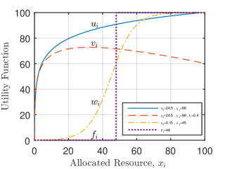
Figure 1: Utility functions: normalized logarithmic (strictly-increasing concave) utility function $u_{i}$ and corresponding nonmonotonous payoff functions $v_{i}$ when $L=0.4$, as well as a discontinuous Step utility function $f_{i}$ and corresponding approximate continuous Sigmoidal utility function $w_{i}\,$.

Figure 2: *

(a)

Figure 3: *

(b)

Figure 4: Resource allocation solution approaches, (a) centralized , (b) distributed iterative.

In this paper, we propose a distributed and iterative algorithm, that is a computationally efficient and private solution of the resource allocation problems. A stochastic version of the algorithm was used for common goods such as clean air and access to public road in [27]. We extend the applications and we make the following specific contributions. We propose derandomized version of AIMD algorithm to allocate common goods to users with strictly increasing, concave utility functions. We also propose AIMD algorithm to allocate subsidized goods, where the fee per use is shared with the entire population, to users with concave and nonmonotonous utility functions. We extend the results to propose a variant of AIMD algorithm to allocate common goods to users with Sigmoidal utility functions.
The rest of this paper is organized as follows. Section 2 presents the problem formulation. In section 3, we propose variants of AIMD distributed algorithm for allocation of subsidized (and common) goods among users based on their specific utility functions. Section 4, includes EV charging simulation setup and discuss the numerical results. Section 6 concludes the paper.

2 Distributed Resource Allocation

In this section, we formally define resource allocation problem using utility function concept for both centralized and distributed solution approaches. The objective is to determine each user’s optimal allocated resource at which maximum total utility is achieved.

Remark 1.

In real life applications, the resource could be time-slotted like energy in $\mathrm{k}\mathrm{W}\mathrm{h}$ or time-varying like power in $\mathrm{k}\mathrm{W}$. Although, we consider a time-slotted optimization problem, we can use the proposed solution for any time-varying situations without changing the results.

2.1 Baseline and Problem Formulation

Consider $n$ users utilize a shared limited resource $C>0$, and let $x_{i}\geq 0$ represents the possible allocated resource to each user $i=1,\dots,n$. We attribute a utility, i.e., a measure of satisfaction, to each user $i$ who takes advantage of the common resource and describe it by means of a utility function. The utility function $u_{i}:\mathbb{R}_{+}\rightarrow\mathbb{R}_{+}$, assigns a non-negative real number to each possible value of allocated resource $x_{i}$, to represent the level of satisfaction for each user $i$ or quality of service (QoS).
A class of centralized resource allocation problems can be formulated as a nonlinear continuous optimization problem (1) that is also represented in Figure 4a. In such problems, a central decision maker calculates the optimal solution vector $\textbf{x}^{*}=[x_{1}^{*},...,x_{n}^{*}]^{\top}$, by collecting all information regarding each user’s utility function $u_{i}$, capacity constraint $C$, and number of users $n$. Although centralized solution approaches focus to determine efficient resource allocation, in many realistic applications, it is neither applicable nor desirable [18] since it violates users’ privacy.
Figure 4(b) depicts a class of distributed (and iterative) approach to resource allocation problems in which allocations emerge as the result of an iterative of local procedures. In other words, a set of users locally make decisions regarding their resources autonomously. To this end, an algorithm is used to assign each user $i$ an allocated resource $x_{i}{(t)}$ in time steps (iterations) ${1,\dots,t}$. In each iteration, each user’s algorithm update user’s allocated resource $x_{i}{(t)}$ locally by choosing one of these options: increase, decrease or no-change compared with previous iteration $x_{i}{(t-1)}$. The increase option continues until receiving one bit signal $s{(t-1)}$, that notify capacity constraint $\sum_{i=1}^{n}{x_{i}{(t)}}>C$ is violated and algorithm, based on a certain probability, choose one of the following options: decrease or no-change. When the capacity is available again $\sum_{i=1}^{n}{x_{i}{(t)}}\leq C$, the increase option of the algorithm restarts immediately. The procedure repeats until the number of iterations is large enough $t$, and users’ allocated resource converge to the optimal allocation $x^{*}$.
In order to quantify efficiency of distributed resource allocation, we express the efficiency as follows:

$$\text{efficiency at time }t=\frac{\lim_{t\rightarrow\infty}\sum_{i=1}^{n}{u_{i}(x_{i}(t))}}{\sum_{i=1}^{n}{u_{i}(x_{i}^{*})}}\,,\\$$ (2)

where the numerator is the output of proposed distributed algorithm and the denominator is the solution of an interior-point optimization algorithm. In the following sections, we show that the efficiency converges to $1$.

3 AIMD Algorithm

In this section, we describe several variants of AIMD algorithm.

Remark 2.

AIMD (Additive Increase Multiplicative Decrease) is a distributed and iterative algorithm that is used widely to control congestion in computer networks. The objective of AIMD is to determine the share of the resource for each user while total demands remains less than the available capacity, and where the limited communication in the network is desired. The AIMD algorithm, in its basic version, is composed of two procedures. In the additive increase (AI) phase, users continuously request for more available resource of the network until receiving a notification that the aggregate amount of available resource has been exceeded. Then the multiplicative decrease (MD) phase occurs and users respond to the notification by reducing their share proportionally. The AI phase of the algorithm restarts again immediately and this pattern is repeated by each active user in the network [6].

For the sake of representation, we reproduce the stochastic allocated-dependent version of AIMD algorithm that is used for allocation of common goods among users with concave and strictly increasing utility functions. We shall not describe the guaranties of the algorithm here, rather we refer the interested readers to [27] for details. Thus, we consider a further and substantial assumption, so-called concavity assumption, for users utility functions which provide mathematical tractability of optimization problem (1).

Assumption 1.

(Concavity Assumption) The utility functions $u_{i}:\mathbb{R}_{+}\rightarrow\mathbb{R}_{+}$, (i) are strictly increasing functions of $x_{i}$ with $u_{i}(0)=0$, (ii) are concave and continuously diffrentiable with domain $x_{i}\geq 0$, where $x_{i}$ is the amount of resources allocated to user $i$.

Example 2.

We use normalized logarithmic function Equation (3) as strictly increasing concave utility function that satisfies Concavity Assumption 1 in order to model the level of satisfaction of EV owners whose car is connected to the charging station to be charged.

$$u_{i}(x_{i})=100\frac{\log(1+\eta_{i}x_{i})}{\log(1+\eta_{i}\chi_{i})}\,,$$ (3)

where $\chi_{i}$ in $\mathrm{k}\mathrm{W}\mathrm{h}$ is the amount of allocated resource (EV charging) that gives $100$ unit utility to the user $i$. It also satisfies $u_{i}(0)=0$. The parameter $\eta_{i}$ indicates how the charge needed urgently by effecting on the rate of utility percentage that is a function of allocated resource $x_{i}$. Intuitively higher values of $\eta_{i}$ yield higher utility to user $i$. Figure 1 represents a normalized logarithmic utility functions $u_{i}$ with $\eta_{i}=24.5,~{}\chi_{i}=98$.

In AI phase, each active user $i$ continues to update its allocated resource $x_{i}{(t)}$ upward by adding an amount of growth factor $\alpha\in(0,C)$ to its previous allocated resource $x_{i}{(t-1)}$ while $\sum_{i=1}^{n}{x_{i}\leq C}$. When the capacity limit has been violated, i.e., $\sum_{i=1}^{n}{x_{i}>C}$, users are notified to execute MD phase. Each user will respond to the capacity signal independently with a certain probability $\lambda_{i}\,$, by multiplying the previous allocated resource $x_{i}{(t-1)}$ to a drop factor $\beta\in(0,1)$ to form current allocated resource $x_{i}{(t)}$. The probability $\lambda_{i}$ at $t$-th iteration, for each user $i$, depends on the long-term average allocated resource $\bar{x}_{i}{(t)}=\frac{1}{t+1}\sum_{k=1}^{t}{x_{k}}$ through the relation $\lambda_{i}(\bar{x}_{i}{(t)})=\Gamma\frac{u^{\prime}_{i}(\bar{x}_{i}{(t)})}{\bar{x}_{i}{(t)}}$, where the parameter $\Gamma$ is chosen to ensure that $0<\lambda_{i}(\bar{x}_{i})<1$.

Algorithm 1 AIMD for user $i$

1:Initialize $x_{i}{(0)}$ arbitrary

2:Broadcast the parameter $\Gamma$

3:for time steps $t=1,2,3,\dots$ do

4:     if $\sum_{j=1}^{n}{x_{j}{(t)}}<C$ then

5:          $x_{i}{(t+1)}=x_{i}{(t)}+\alpha$;

6:     else

7:          $x_{i}{(t+1)}=\beta x_{i}{(t)}$ with probability $\lambda_{i}(\bar{x}_{i}{(t)})=\Gamma\frac{u^{\prime}_{i}(\bar{x}_{i}{(t)})}{\bar{x}_{i}{(t)}}$

8:          $x_{i}{(t+1)}=x_{i}{(t)}$ otherwise;

9:     end if

10:end for

3.1 Derandomized Algorithm

The proposed stochastic AIMD Algorithm 1 is considered to have access to sources of perfect randomness, i.e. unbiased and completely independent random variables, however in real-world implementation, the physical sources of randomness to which we have access may contain biases and correlations [26]. Thus, the probabilistic method can also yield insight into how to construct deterministic algorithms [19]. We now propose a variant of deterministic AIMD for the same purpose.

Algorithm 2 DAIMD for user $i$

1:Initialize $x_{i}{(0)}$ arbitrary

2:Broadcast the parameter $\Gamma$

3:for time steps $t=1,2,3,\dots$ do

4:     if $\sum_{j=1}^{n}{x_{j}{(t)}}<C$ then

5:         $x_{i}{(t+1)}=x_{i}{(t)}+\alpha$;

6:     else

7:         $\lambda_{i}(\bar{x}_{i}{(t)})=\Gamma\frac{u^{\prime}_{i}(\bar{x}_{i}{(t)})}{\bar{x}_{i}{(t)}}$,

8:         $x_{i}{(t+1)}=\beta(1-\lambda_{i})x_{i}{(t)}+\lambda_{i}x_{i}{(t)}$;

9:     end if

10:end for

We show that the strong convergence of derivative of utility function of long-term average allocated resource $u^{\prime}_{i}(\bar{x}_{i}{(t)})$, can be used to allocate resource optimally. Therefore, there exists a derandomized algorithm with the same performance as the randomized algorithm.
We define a vector $z(t)$ consists of $d\in\mathbb{N}$ real-valued elements by

$$z(t):=[x_{1}\,\dots\,x_{n}\ \bar{x}_{1}\ \dots\,\bar{x}_{n}\ \lambda_{1}\,\dots\,\lambda_{n}]^{\top},$$ (4)

and let a class $\{f^{(t)}:\mathbb{R}^{d}\rightarrow\mathbb{R}^{d},t=1,2,\dots\}$ of functions such that

$$z(t)=f^{(t)}(z(t-1)).$$ (5)

Each function $f_{\ell}^{(t)}:\mathbb{R}^{d}\rightarrow\mathbb{R}$, $\ell=1,\dots,d$ is also considered …
The allocated resource $x_{i}(t)$ at $t$-th iteration, for each user $i$, is calculated as Equations (6).

$$\begin{split}x_{i}(t)=(x_{i}(t-1)+\alpha)\mathds{1}_{[\sum_{j=1}^{n}{x_{j}{(t)}}<C]}+(\beta(1-\lambda_{i})x_{i}{(t)}\\ +\lambda_{i}x_{i}{(t)})\mathds{1}_{[\sum_{j=1}^{n}{x_{j}{(t)}}\geq C]}\end{split}$$ (6)

$$\bar{x}_{i}{(t)}=\frac{1}{t+1}\sum_{k=1}^{t}{x_{k}}$$ (7)

Therefore, iterated function systems (IFS) is defined as: We define $\lambda_{i}(\bar{x}_{i}{(t)})=\Gamma\frac{u^{\prime}_{i}(\bar{x}_{i}{(t)})}{\bar{x}_{i}{(t)}}$ and we use it in MD phase of the algorithm by $x_{i}{(t+1)}=\beta(1-\lambda_{i})x_{i}{(t)}+\lambda_{i}x_{i}{(t)}$ to build DAIMD Algorithm 2.

3.2 Subsidized Goods

We extend resource allocation problem to subsidized goods where the fee per use is shared with the entire population. Suppose if each user $i$ is charged a constant price $L$ per unit of the received resources $x_{i}$. Each user payoff function, $v_{i}:\mathbb{R}_{+}\rightarrow\mathbb{R}_{+}$ is defined as utility function minus the cost of received resource as follows:

$$v_{i}(x_{i})=u_{i}(x_{i})-Lx_{i}\,.$$ (8)

Recall each user utility function $u_{i}(x_{i})$ is considered under Concavity Assumption 1, therefore, each user payoff function (8) is a concave function but it is not necessarily increasing. The centralized resource allocation problem can then be formulated as follows:

$$\underset{x_{1},\dots,x_{n}}{\text{maximize}} \sum_{i=1}^{n}{v_{i}(x_{i})}$$ (9)

subject to $$\sum_{i=1}^{n}{x_{i}\leq C}\,,$$

$$x_{i}\geq 0\;,\;i=1,\dots,n\,.$$

The optimization problem 9 in which the objective function is non-negative sum of concave functions, is concave and there exists a global optimal solution [3].

Example 3.

Suppose normalized logarithmic function Equation (3) to show each EV owner’s satisfaction from receiving an amount of energy allocation $x_{i}\,$. The cost of allocated energy is defined as the price of energy $L$ in monetary units, multiply in energy allocation $x_{i}\,$. Therefore, the payoff function is defined as follows:

$$v_{i}(x_{i})=100\frac{\log(1+\eta_{i}x_{i})}{\log(1+\eta_{i}\chi_{i})}-Lx_{i}\,.$$ (10)

Figure 1 represents a normalized logarithmic utility function with $\eta_{i}=24.5~{},~{}\chi_{i}=98$ compared with corresponding payoff functions $v_{i}$ when $L=0.4\,$.

We improve AIMD Algorithm 1 by controlling the allocation do not exceed from maximum payoff of each user and design the PAIMD Algorithm 3. The control is applied locally since each user $i$ calculates the optimal point $x_{i}^{*}=\textstyle\operatorname*{arg\,max}_{x_{i}\in\mathbb{R}_{+}}v_{i}(x_{i}),\ \forall i=1,\dots,n$ and then in each iteration, in the (AI) phase of the algorithm compare it to allocated resource $x_{i}{(t)}+\alpha$ to choose the minimum allocation.

Algorithm 3 PAIMD for user $i$

1:Initialize $x_{i}{(0)}$ arbitrary

2:Each user $i$ calculates $x_{i}^{*}=\displaystyle\operatorname*{arg\,max}_{x_{i}\in\mathbb{R}_{+}}\ v_{i}(x_{i}),\ \forall i=1,\dots,n$

3:Broadcast the parameter $\Gamma$

4:for time steps $t=1,2,3,\dots$ do

5:     if $\sum_{j=1}^{n}{x_{j}{(t)}}<C$ then

6:          $x_{i}{(t+1)}=\min(x_{i}^{*}\;,\;x_{i}{(t)}+\alpha)$

7:     else

8:          $x_{i}{(t+1)}=\beta x_{i}{(t)}$ with probability $\lambda_{i}(\bar{x}_{i}{(t)})=\Gamma\frac{v^{\prime}_{i}(\bar{x}_{i}{(t)})}{\bar{x}_{i}{(t)}}$

9:          $x_{i}{(t+1)}=x_{i}{(t)}$ otherwise;

10:     end if

11:end for

Based on $\chi_{i}and\eta_{i}$, define bounded value

3.3 Sigmoidal Utility Functions

In this section, we model resource allocation problem (1) using Sigmoidal users’ utility functions that is defined as following:

Definition 1.

The utility function of $w_{i}:\mathbb{R}_{+}\rightarrow\mathbb{R}_{+}$ is defined to be Sigmoidal if: (i) The $w_{i}(0)=0$ and $w_{i}$ is strictly increasing function of $x_{i}$. (ii) $w_{i}(x_{i})$is continuously differentiable, with domain $x_{i}\geq 0$. (iii) $w_{i}(x_{i})$is convex for $x_{i}\leq\psi_{i}$ and is concave for $x_{i}\geq\psi_{i}$, which $\psi_{i}\in\mathbb{R}_{+}$ is the inflection point.

Algorithm 4 QAIMD for user $i$

1:Initialize $x_{i}(0)$ arbitrary

2:Broadcast the parameters $\Gamma_{1}$, $\Gamma_{2}$

3:for time steps $t=1,2,3,\dots$ do

4:     if $\bar{x}_{i}(t)<\psi_{i}$ then

5:         if $\sum_{j=1}^{n}{x_{j}(t)}<C$ then

6:              $x_{i}(t+1)=\frac{1}{\beta}x_{i}(t)$ with probability $\lambda_{i}=\Gamma_{1}\frac{w^{\prime}_{i}(\bar{x}_{i}(t))}{\bar{x}_{i}(t)}$

7:              $x_{i}(t+1)=x_{i}(t)$ otherwise;

8:         else

9:              $x_{i}(t+1)=\max(0\;,\;x_{i}(t)-\alpha)$

10:         end if

11:     else

12:         do AIMD with $\alpha$, ${\beta}$ and probability $\lambda_{i}=\Gamma_{2}\frac{w^{\prime}_{i}(\bar{x}_{i}(t))}{\bar{x}_{i}(t)}$

13:     end if

14:end for

Example 4.

(Why do we need Sigmoidal utility functions?). In some situations, such as charging an electric vehicle with the goal of reaching a predetermined destination (e.g., airport, home, etc.), the user receive negligible (or non) utility until a threshold of resource is reached (e.g., enough electric charge to arrive at the destination). Ideally, the best description of the utility function is through a discontinuous Step function as follows:

$$f_{i}(x_{i})=\begin{cases}0&\text{if $x_{i}<\theta_{i}$}\,;\\ 100&\text{if $x_{i}\geq\theta_{i}$}\,,\end{cases}$$ (11)

where $\theta_{i}$ shows the sufficient allocated resource that gives 100 unit utility to user $i$.
Continious Sigmoidal utility functions may be used to approximate a step utility function to any arbitrary accuracy [25]. Thus, we model EV owner’s satisfaction with Sigmoidal utility function that is expressed by:

$$w_{i}(x_{i})=\frac{100}{1+e^{-\eta_{i}(x_{i}-\psi_{i})}}-\frac{100}{1+e^{\eta_{i}\psi_{i}}}\,,$$ (12)

where $\eta_{i}$ is the steepness of the curve that indicates how the charge is needed urgently for each user $i$. The parameter $\psi_{i}$ in $\mathrm{k}\mathrm{W}\mathrm{h}$ is the inflection point that achieving it satisfies the urgent need of user $i$. The function, also, satisfies $w_{i}(0)=0$ and $\lim_{x_{i}\to+\infty}w(x_{i})\approx 100$. Figure 1 represents a Step utility function $f_{i}$ with $\theta_{i}=48$ and an approximate corresponding Sigmoidal utility function $w_{i}$ with $\eta_{i}=0.15$ and $\psi_{i}=45\,$.

The QAIMD Algorithm 4 represents the procedure of allocation among users with Sigmoidal utility functions. The key point is that in each iteration $(t)$, the long-term of allocated resource $\bar{x}_{i}(t)$ is compared with each user $i$’s inflection point $\psi_{i}$. If $\bar{x}_{i}(t)<\psi_{i}$, the increase phase is built by multiplying the previous state $x_{i}(t)$ in a growth factor $\frac{1}{\beta}>1$ to construct current state $x_{i}(t+1)$ with a probability $\lambda_{i}(\bar{x}_{i}(t))=\Gamma_{1}\frac{w^{\prime}_{i}(\bar{x}_{i}(t))}{\bar{x}_{i}(t)}$. The decrease phase also is made by subtracting $\alpha$ from the previous state. When $\bar{x}_{i}(t)\geq\psi_{i}$, the algorithm is work with AIMD Algorithm 1 procedure. Note that there are two parameters $\Gamma_{1}$, $\Gamma_{2}$ to ensure $0<\lambda_{i}(\bar{x}_{i})<1$ in each case.

4 Simulation

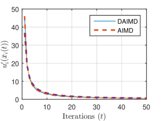
(a)

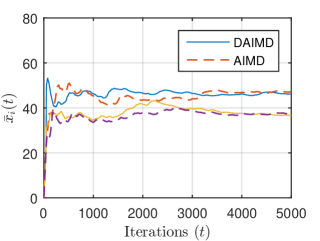
(b)

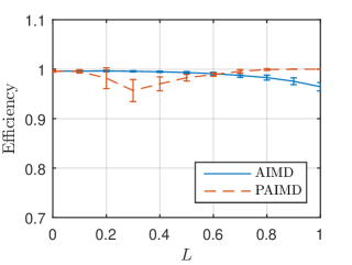
(c)

Figure 5: LABEL:sub@fig:Duprime_xbar_t_compare The deterministic derivative of payoff function $u^{\prime}_{i}(\bar{x}_{i}{(t)})$ for two randomly selected users (solid lines) compared with corresponding stochastic ones (dashed lines), LABEL:sub@fig:Dxbar_t_compare the deterministic average of allocated resource $\bar{x}_{i}{(t)}$ to the stable point for two randomly selected users (solid lines) compared with corresponding stochastic ones (dashed lines), LABEL:sub@fig:Efficiency the efficiency of AIMD Algorithm 1 and PAIMD Algorithm 3 for $L\in\{0,0.1,\dots,1\}$ calculated by Equation (2).

In order to figure out the effectiveness, the AIMD Algorithm 2, 3 and 4 was applied to various logarithmic and Sigmoidal utility functions with different parameters in MATLAB.
The resource allocation domain is considered as a charging station whose power supplies from renewable energy (e.g. solar or wind), with constant capacity in $\mathrm{k}\mathrm{W}\mathrm{h}$ equal to $C=35\%$ of the sum of users utility functions when each user receives $100$ unit satisfaction. The users $n=50$ are the EV owners who connected their vehicles to the station for charging at the same time. The AIMD parameters are identical for all users with $\alpha=1$ and $\beta=0.85$. The parameter $\Gamma$ is also chosen to assure us the condition $\lambda_{i}(\bar{x}_{i})\in(0,1)$ is satisfied.

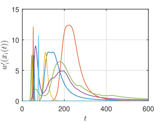
(a)

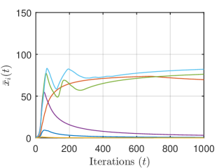
(b)

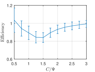
(c)

Figure 6: LABEL:sub@fig:wprime_xbar_t The derivative of Sigmoidal utility functions $w^{\prime}_{i}(\bar{x}_{i}{(t)})$ for six randomly selected users when $C/\Psi=1.5$, LABEL:sub@fig:wxbar_t the average of allocated resource $\bar{x}_{i}{(t)}$ to the stable point for six randomly selected users when $C/\Psi=1.5$, LABEL:sub@fig:Efficiency the efficiency of QAIMD Algorithm 4 calculated by Equation (2).

First, we adopt normalized logarithmic utility function expressed by (3), as a strictly increasing concave function which satisfies Concavity Assumption 1. We choose $\chi_{i}$ independent uniformly distributed random number with support $(40,60)$ and $\eta_{i}$ independent uniformly distributed random number with support $(0,1)$.
We apply deterministic DAIMD Algorithm 2 for allocation of power as a common good (no charging fee) to EVs connected to the charging station. Figure 5a shows a rapid convergence for derivative of payoff functions $u^{\prime}_{i}(\bar{x}_{i}(t))$ when iteration $t$ increases. It also reveals the coincidence of deterministic and stochastic versions of derivative of payoff functions $u^{\prime}_{i}(\bar{x}_{i}(t))$. Figure 5b depicts the value of long-term average state $\bar{x}_{i}(t)$ for two randomly selected users and shows each of them converge to a stable value. It also represents that deterministic and stochastic version of average state $\bar{x}_{i}(t)$ fluctuate differently but the long-term averages for each user converge to optimal allocation. The efficiency of deterministic DAIMD Algorithm 2, calculated by Equation (2), in different runs are a real number in the range of $(0.97,0.99)$.
We also apply stochastic PAIMD Algorithm 3 for allocation of power as a subsidized good to EVs connected to charging station. Therefore, we consider the price per unit $L\in\{0.1,0.2,\dots,1\}$ of the power $x_{i}$ in the payoff function (10). Figure 5c, depicts the efficiency of PAIMD Algorithm 3 compared with AIMD Algorithm 1, both calculated by Equation (2). The efficiency of PAIMD Algorithm 3 decreases when the value of $L$ increases until receiving to a minimum value in ($L=0.3$). For large values of $L>0.3$ the efficiency of PAIMD Algorithm 3 increases and converge to $1$.
Second, we model EV owner satisfaction with Sigmoidal utility function that are expressed by Equation (12). We choose $\psi_{i}$ independent uniformly distributed random number with support $(25,100)$ and $\eta_{i}$ independent uniformly distributed random number with support $(0,25)$. The parameter $\Gamma_{1}$ and $\Gamma_{2}$ is also chosen to assure us the condition $\lambda_{i}(\bar{x}_{i})\in(0,1)$ is satisfied. Figure 6a depicts the derivative of utility functions $w^{\prime}_{i}(\bar{x}_{i}{(t)})$ for six randomly selected users. It illustrates that the derivatives approach to zero as $t$ increase but the convergence is slower than the derivatives of logarithmic utility function $v^{\prime}_{i}(\bar{x}_{i}{(t)}$ in Figure 5a . In Figure 6b the average of allocated resource $\bar{x}_{i}{(t)}$ for six randomly selected users is displayed. It shows $\bar{x}_{i}{(t)}$ approach to a constant value for some users and to $0$ for some other users.
Figure 6c represents the efficiency of QAIMD 4, calculated by Equation (2), for different capacity $C/\Psi=\{0.5,0.75,\dots,3\}$, where $\Psi=\sum_{i=1}^{n}{\psi_{i}}$. For each user $i$ the algorithm decides between increasing allocated resource or decreasing it toward zero. The efficiency of the algorithm is better for small values of capacity constraint, but it decrease when capacity is around $\Psi$. The efficiency improve again when $C/\Psi$ is large enough.

5 Loss of Efficiency Due to Competition

In this section, we allow the individual users to act strategically as in a game. We consider a game in strategic form, where all users’ utility functions are common knowledge. The resulting competition over a scarce resource is reminiscent of the tragedy of the commons . An user may deviate from the AIMD algorithm and strategically request more resource in order to improve its payoff. Alternatively, an user may follow the AIMD algorithm but mispresent its utility function. However, we show that, in some situations, the AIMD outcome and the game’s Nash equilibrium are close to each other.

5.1 Resource Allocation as a Strategic Game

Imagine a resource allocation problem in which there are $n$ users, competing to utilize a scarce fixed common resource of $C>0$. Each user $i$ chooses his own consumption of resources $x_{i}$ from a set of action space $X_{i}=\{x_{i}\in\mathbb{R}\ |\ 0\leq x_{i}\leq C\}$. A profile of actions $x=(x_{i},x_{-i})$ describe a particular combination of actions chosen by all users, where $x_{-i}\in X_{-i}$ is a particular possible of actions for all players who are not $i$.

Consuming an amount $x_{i}\geq 0$ gives user $i$ a benefit equal to $u_{i}(x_{i})$ when ${\sum_{j=1}^{n}{x_{j}}\leq C}$ and intuitively no other users benefits from $i$’s choice. When $x_{i}$ increases or other users consume more resources so that $\sum_{j=1}^{n}{x_{j}}>C$, the user get nothing $u_{i}(x_{i})=0$ because additional requested resources are not provided. Then we define the payoff function $\tilde{u}_{i}(x_{i},x_{-i})$ of a user $i$ from a profile of actions $x$ as

$$\tilde{u}_{i}(x_{i},x_{-i})=\begin{cases}u_{i}(x_{i})&\text{if $\sum_{j=1}^{n}{x_{j}}\leq C$}\,;\\ 0&\text{if $\sum_{j=1}^{n}{x_{j}}>C$}\,.\end{cases}$$ (13)

Where the utility function $u_{i}(x_{i})$ is considered to be concave, strictly increasing, and continuously differentiable ,i.e., follows assumption 1.

The strategic game $(\mathcal{N},X_{i},\tilde{u_{i}})_{i\in\mathcal{N}}$, that have infinitely many pure strategies but utility functions are not continuous, is discontinuous infinite strategic games. This problem should be consider precisely because it may lead to problem of nonexistence of unique Nash equilibrium.

5.2 Nash Equilibrium

To cut to the chase, the key notion to solve the strategic game $(\mathcal{N},X_{i},\tilde{u_{i}})_{i\in\mathcal{N}}$, is the Nash equilibrium, that is an outcome (a decision made by each player) such that no player can improve his individual payoff through an unilateral move. As stable situations, Nash equilibrium are often considered to be the expected outcomes from interactions. To solve for a Nash equilibrium we compute the best-response function correspondence for each player and then find an action profile for which all best-response functions are satisfied together.

To find a solution for Equation (13), we first write out each player $i$’s best-response correspondence and we consider that given $x_{-i}$, player $i$ will want to choose an element in $BR_{i}(x_{-i})$. Given $x_{-i}\in X_{-i}$ each player $i$’s best response is the difference between $C$ and $\sum_{j\neq i}^{n}{x_{j}}\,$. If user $i$ asks for more, then all users get nothing while if asks for less then he is leaving some resources unclaimed and therefore

$$BR_{i}(x_{-i})=C-\sum_{j\neq i}^{n}{x_{j}}\,.$$ (14)

It is easy to see from the best response correspondence that any profile of demands $x_{i}\in[0,C]$ that add up to $C$ will be a Nash equilibrium. Hence, each player $i$ is indifferent between all of his requests $x_{i}\in[0,C]$ and the game is just not blessed with a unique equilibrium and has an infinite number of equilibria. The obvious problem with multiple equilibria is that the players may not know which equilibrium will prevail. Hence, it is entirely possible that a non-equilibrium outcome results because one player plays one equilibrium strategy while a second player chooses a strategy associated with another equilibrium [4].

It turns out that resource allocation encounters conflict over scare resources that results from the tension between individual selfish interests and common good. As Hardin stated in his article [10], “freedom in a commons brings ruin to all,” that here means, social utility of an uncontrolled use of the common resources that each user have the freedom to make choices, is worse than if those choices were regulated. This results in the occurrence of the phenomenon called tragedy of the commons. In fact, individual users acting independently according to their own self-interest behave contrary to the common good of all users by depleting that resource through their collective actions.

To solve this problem, we first need to bring back the continuity to the payoff function Equation (13). Thus, we apply the resource allocation back-off condition $\sum_{j=1}^{n}{x_{j}}>C$ directly to the payoff function for each user $i$. We define a concave penalty function ${\tau:\mathbb{R}_{+}\rightarrow\mathbb{R}_{+}}$ so that $\tau(0)=1$ and $\tau(C)=0$ and multiply it to the payoff function (13). To generalize, we also consider each unit of resource costs $L$ and we have

$$\tilde{v}_{i}(x_{i},x_{-i})=u_{i}(x_{i})\,\tau\Big{(}\sum_{j=1}^{n}{x_{j}}\Big{)}-Lx_{i}\,,$$ (15)

$$\textrm{for all}\quad x_{i},x_{j}\in[0,\infty)\,.$$

Example 5.

Consider, for example, the concave penalty function $\tau(z)$ as follows:

$$\tau\Big{(}z\Big{)}=\sqrt{1-\frac{z^{p}}{C^{p}}}\,\ ,$$ (16)

where $z=\sum_{j=1}^{n}{x_{j}}$ and $p\in\mathbb{N}$. Intuitively, $\tau(0)=1$ and $\tau(C)=0$.

Figure 7 represents some examples of concave penalty functions Equation (16) for $p\in\{1,2,4,8\}$. Although the larger values of $p$ reduce inefficiency of Nash equilibrium, however make calculations more complex. In realistic situation of EV charging, this function can be programmed to the charger and it works when the demand exceeds from capacity $C$.

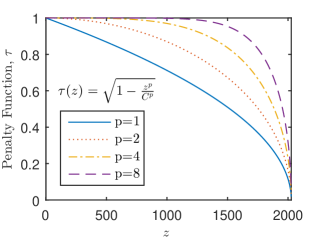
Figure 7: Penalty Function

Since the payoff functions are continuous there is a strong result on existence of the pure Nash equilibrium that is stated by Theorem 1 [7].

Theorem 1.

(Debreu, Glicksberg, Fan) An infinite strategic form game $\mathcal{G}=(\mathcal{N},X_{i},f_{i})_{i\in\mathcal{N}}$ such that for each $i\in\mathcal{G}$ (i) $X_{i}$is compact and convex; (ii) $f_{i}(x_{i},x_{-i})$is continuous in $x_{-i}$; (iii) $f_{i}(x_{i},x_{-i})$is continuous and concave in $x_{i}$ . Then a pure strategy Nash equilibrium exists.

Another important question that arises in the analysis of strategic form games is whether the Nash equilibrium is unique. Theorem 2, provides sufficient conditions for uniqueness of an equilibrium in games with infinite strategy sets.

Theorem 2 (Theorem 1, [20]).

Consider a strategic form game $\mathcal{G}=(\mathcal{N},X_{i},f_{i})_{i\in\mathcal{N}}$ . For all $i\in\mathcal{G}$, assume that the action sets $X_{i}=\{x_{i}\in\mathbb{R}^{m_{i}}|h_{i}(x_{i})\geq 0\}$, where $h_{i}$ is a concave function, and there exists some $\tilde{x}\in\mathbb{R}^{m_{i}}$ such that $h_{i}(\tilde{x}_{i})>0$ . Assume also that the payoff functions $(f_{i})_{i\in\mathcal{N}}$ are diagonally strictly concave for $x\in X$ . Then the game has a unique pure strategy Nash equilibrium. Where payoff functions $(f_{i})_{i\in\mathcal{N}}$ are diagonally strictly concave for $x\in X$, if for every $x^{ne},\bar{x}\in X$, we have $(\bar{x}-x^{ne})^{\top}\nabla f(x^{ne})+(x^{ne}-(\bar{x})^{\top}\nabla f(\bar{x})>0$ .

The game $(\mathcal{N},X_{i},\tilde{v}_{i})_{i\in\mathcal{N}}$ has unique Nash equilibrium that is calculated by maximizing user $i$’s payoff function $\tilde{v}_{i}(x_{i},x_{-i})$ and finding the solution to the first order conditions. So, we write down the first-order condition of user $i$’s payoff function as follows

$$x_{i}^{ne}=\frac{\partial\tilde{v}_{i}(x_{i},x_{-i})}{\partial x_{i}}=0\,.$$ (17)

We therefore have $n$ such equations, one for each player, and the unique Nash equilibrium is the strategy profile $x^{ne}$ for which all users in the network, the Equation 17 are satisfied together, so that

$$x^{ne}=(x_{i}^{ne},x_{-i}^{ne}),\ x_{i}^{ne}=\displaystyle\operatorname*{arg\,max}_{x_{i}\in[0,C]}\ \tilde{v}_{i}(x_{i},x_{-i}),\ \forall i\in\mathcal{N}\,.$$ (18)

When resource allocation problem form as a result of selfish competition among users, the resulting stable solution may not, in fact, be system optimal [16]. In this circumstance, we would like to measure inefficincy constituted due to decentralized control. This is very important to decide whether a decentralized mechanism can be applied, regarding the loss of efficiency in comparison with the performance that would be obtained with a central authority. Price of anarchy (PoA)  [13], is a concept that quantifies this inefficiency and is measured as the ratio between the worst equilibrium and the centralized solution. In the problem considered here, this notion will be slightly different and defined as the efficiency of the unique Nash equilibrium of the game $\mathcal{G}=(\mathcal{N},X_{i},f_{i})_{i\in\mathcal{N}}$ and the optimal centralized solution of (10) as follows:

$$PoA=\frac{\sum_{i=1}^{n}{\tilde{v}_{i}(x_{i}^{ne})}}{\sum_{i=1}^{n}{v_{i}(x_{i}^{*})}}\,,\\$$ (19)

where $x^{ne}$ is the unique Nash equilibrium given by (18) and $x^{*}$ is the solution of (10) .

5.3 Simulation

In this section, we proceed to simulate resource allocation in competition game to investigate in more details the inefficiency of Nash equilibrium. For this purpose, suppose the EV charging station settings of the section LABEL:Sec:AIMD_Numerical_Simulation. Each user’s utility function is considered as the normalized logarithmic function (3) with uniformly distributed random parameters of $\eta_{i}\in(0,25)$ and $\chi_{i}\in(25,100)$. We also consider the concave penalty function Equation 16 with $p=1$ for executing the simulation. We start to simulate the problem for two players. Consider the charging station with the limited resource of $C=25$ $\mathrm{k}\mathrm{W}\mathrm{h}$ and two EV owners $i\in\{1,2\}$ which their EVs are connected to the station for charging. Both players have normalized logarithmic utility function Equation (3) with parameters $\eta_{1}=15$, $\chi_{1}=30$ and $\eta_{2}=38$, $\chi_{2}=70$ respectively. Figure LABEL:fig:contour_Csmall_tau depicts inefficiency of distributed competitive resource allocation in two-player game ,i.e., best response functions lines intersection, compared with optimal solution $U(x_{1}^{*},x_{2}^{*})$.

Now consider the same setting for a charging station with $n=50$ users. Figure plots social optimum of Nash equilibrium $\sum_{i=1}^{n}{\tilde{v}_{i}(x_{i}^{ne})}$, compared with optimal centralized solution $\sum_{i\in\mathcal{N}}{v_{i}(x_{i}^{*})}$ for diffrent $L=\{0,0.1,\dots,1\}$. Figure 8 represents the price of anarchy in competition against two parameters of price and number of users. The PoA is so sensitive to number of users in the competition such that increasing number of users negatively affect on PoA. Moreover, if the selfish behavior of users in competition do not control by pricing, inefficiency increase and consequently the PoA decrease. Note that the price of anarchy is independent of the competition topology [21].

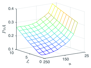
Figure 8: Price of Anarchy (PoA)

5.4 Related Work

Both centralized and distributed solution approaches for the generic problem of resource allocation were studied widely in various fields of expertise and a full review is impossible here. In data networks, that the optimization problem called Network Utility Maximization (NUM), users utility functions are commonly considered to be concave, continuous and strictly increasing functions modeling elastic networks [12], [22], which are more mathematically tractable [3], but limits applicability. Many other applications require inelastic network that are more challenging, where non-concave or discontinuous utility functions need to be maximized. Inelastic networks studied in [15], [8], [9] and Sigmoidal programming algorithm is proposed in [25]. In [1], using utility proportional fairness policy, both elastic and inelastic utility functions compared.
There is also substantial literature on AIMD, the algorithm proposed in [5] and applied experimentally in [11], as the most efficient-fair rate control in Internet applications. The efficiency and fairness of the AIMD algorithm also investigated in [14] and a comprehensive review of the AIMD algorithm and its applications is collected in [6]. This work uses the result of [27] that used AIMD algorithm in stochastic framework for common goods resource allocation.
EV charging has been the most widely studied as an application of distributed resource allocation. In [2], proposed a distributed control algorithm that adapts the charging rate of EVs to the available capacity of the network ensuring that network resources are used efficiently and each EV charger receives a fair share of these resources. In [24], proposed a distributed AIMD based algorithm to allocate available power among connected EVs in order to maximize the utilization of EV owners in a range of situations. In [23], they also used the same formalization framework to expand the modifications of the basic AIMD algorithm to charge EVs. In both articles they considered a fairness policy as a constraint. The effectiveness of AIMD at mitigating the impact of domestic charging of EVs on low-voltage distribution networks is investigated [17].

6 Conclusions & Future Work

Our work represents a variety of AIMD-based distributed algorithms for efficient and private resource allocations in real life applications. We considered two type of users’ utility functions based on the application, first strictly increasing concave functions to represent greediness of users and second Sigmoidal functions to describe the utility from goods that are only useful in sufficient quantities. We introduced a stochastic AIMD algorithm to allocate subsidized goods where users have concave and nonmonotonous utility functions. We also proposed derandomized version of AIMD algorithm to allocate common goods to users with strictly increasing utility functions. We extended the results to propose the variant of AIMD algorithm to allocate common resource where users have Sigmoidal utility functions. The numerical simulations of EV charging are also included in order to validate the convergence of our solutions.

References

- [1] A. Abdel-Hadi and C. Clancy. A utility proportional fairness approach for resource allocation in 4g-lte. In Computing, Networking and Communications (ICNC), 2014 International Conference on, pages 1034–1040. IEEE, 2014.
- [2] O. Ardakanian, C. Rosenberg, and S. Keshav. Distributed control of electric vehicle charging. In Proceedings of the fourth international conference on Future energy systems, pages 101–112. ACM, 2013.
- [3] S. Boyd and L. Vandenberghe. Convex optimization. Cambridge university press, 2004.
- [4] G. P. Cachon and S. Netessine. Game theory in supply chain analysis. In Models, Methods, and Applications for Innovative Decision Making, pages 200–233. INFORMS, 2006.
- [5] D. M. Chiu and R. Jain. Analysis of the increase and decrease algorithms for congestion avoidance in computer networks. Computer Networks and ISDN systems, 17(1):1–14, 1989.
- [6] M. Corless, C. King, R. Shorten, and F. Wirth. AIMD dynamics and distributed resource allocation. SIAM, 2016.
- [7] G. Debreu. A social equilibrium existence theorem. Proceedings of the National Academy of Sciences, 38(10):886–893, 1952.
- [8] M. Fazel and M. Chiang. Network utility maximization with nonconcave utilities using sum-of-squares method. In Decision and Control, 2005 and 2005 European Control Conference. CDC-ECC’05. 44th IEEE Conference on, pages 1867–1874. IEEE, 2005.
- [9] P. Hande, S. Zhang, and M. Chiang. Distributed rate allocation for inelastic flows. IEEE/ACM Transactions on Networking, 15(6):1240–1253, 2007.
- [10] G. Hardin. The tragedy of the commons. Journal of Natural Resources Policy Research, 1(3):243–253, 2009.
- [11] V. Jacobson. Congestion avoidance and control. In ACM SIGCOMM computer communication review, volume 18, pages 314–329. ACM, 1988.
- [12] F. Kelly. Charging and rate control for elastic traffic. European transactions on Telecommunications, 8(1):33–37, 1997.
- [13] E. Koutsoupias and C. Papadimitriou. Worst-case equilibria. In Annual Symposium on Theoretical Aspects of Computer Science, pages 404–413. Springer, 1999.
- [14] A. Lahanas and V. Tsaoussidis. Exploiting the efficiency and fairness potential of aimd-based congestion avoidance and control. Computer Networks, 43(2):227–245, 2003.
- [15] J. W. Lee, R.R. Mazumdar, and N.B. Shroff. Nonconvexity issues for internet rate control with multiclass services: stability and optimality. In INFOCOM 2004. Twenty-third AnnualJoint Conference of the IEEE Computer and Communications Societies, volume 1. IEEE, 2004.
- [16] S. Lichter, C. Griffin, and T. Friesz. The calculation and simulation of the price of anarchy for network formation games. arXiv preprint arXiv:1108.4115, 2011.
- [17] M. Liu and S. McLoone. Enhanced aimd-based decentralized residential charging of evs. Transactions of the Institute of Measurement and Control, 37(7):853–867, 2015.
- [18] J. R. Marden and A. Wierman. Distributed welfare games. Operations Research, 61(1):155–168, 2013.
- [19] M. Mitzenmacher and E. Upfal. Probability and computing: Randomized algorithms and probabilistic analysis. Cambridge university press, 2005.
- [20] J. B. Rosen. Existence and uniqueness of equilibrium points for concave n-person games. Econometrica: Journal of the Econometric Society, pages 520–534, 1965.
- [21] T. Roughgarden. The price of anarchy is independent of the network topology. Journal of Computer and System Sciences, 67(2):341–364, 2003.
- [22] S. Shenker. Fundamental design issues for the future internet. IEEE Journal on selected areas in communications, 13(7):1176–1188, 1995.
- [23] S. Stüdli, E. Crisostomi, R. Middleton, and R. Shorten. Aimd-like algorithms for charging electric and plug-in hybrid vehicles. In Electric Vehicle Conference (IEVC), 2012 IEEE International, pages 1–8. IEEE, 2012.
- [24] S. Stüdli, E. Crisostomi, R. Middleton, and R. Shorten. A flexible distributed framework for realising electric and plug-in hybrid vehicle charging policies. International Journal of Control, 85(8):1130–1145, 2012.
- [25] M. Udell and S. Boyd. Maximizing a sum of sigmoids. Optimization and Engineering, 2013.
- [26] S. P. Vadhan et al. Pseudorandomness. Foundations and Trends® in Theoretical Computer Science, 7(1–3):1–336, 2012.
- [27] F. Wirth, S. Stüdli, J. Y. Yu, M. Corless, and R. Shorten. Nonhomogeneous place-dependent markov chains, unsynchronised aimd, and network utility maximization. arXiv preprint arXiv:1404.5064, 2014.
- [28] E. Xydas, C. Marmaras, and L.M. Cipcigan. A multi-agent based scheduling algorithm for adaptive electric vehicles charging. Applied Energy, 177:354–365, 2016.