Chern numbers for the index surfaces of photonic crystals:
conical refraction as a basis for topological materials

Abstract

The classification of bandstructures by topological invariants provides a powerful tool for understanding phenomena such as the quantum Hall effect. This classification was originally developed in the context of electrons, but can also be applied to photonic crystals. In this paper we study the topological classification of the refractive index surfaces of two-dimensional photonic crystals. We consider crystals formed from birefringent materials, in which the constitutive relation provides an optical spin-orbit coupling. We show that this coupling, in conjunction with optical activity, can lead to a gapped set of index surfaces with non-zero Chern numbers. This method for designing photonic Chern insulators exploits birefringence rather than lattice structure, and does not require band crossings originating from specific lattice geometries.

I Introduction

Chern insulators are two-dimensional materials that are insulating in their interior but conducting along their edge. The first such materials to be identified were the integer quantum Hall states Klitzing et al. (1980), for which the quantized Hall conductance corresponds to a topological invariant known as the Chern number Avron et al. (1983); Kohmoto (1985); Thouless et al. (1982). The Chern number is related to the number of conductive edge states at the interface between a topologically non-trivial insulator and a topologically trivial one Hatsugai (1993). A later example of a Chern insulator is provided by the Haldane model Haldane (1988), which introduced a now well-trodden path to constructing topologically non-trivial bandstructures. This model describes particles hopping on a two-dimensional hexagonal lattice, an arrangement which produces point degeneracies in the bandstructure. These are the celebrated Dirac points, which are associated with vortex-like singularities in the Bloch functions. They can be a precursor to a topologically non-trivial gapped bandstructure, which arises if the degeneracies are split by a perturbation in such a way that the windings of the vortices combine rather than cancel Sticlet et al. (2012).

Topologically non-trivial bandstructures are not restricted to theories of electrons, but can also be achieved for photons Raghu and Haldane (2008); Haldane and Raghu (2008); Ochiai and Onoda (2009); Wang et al. (2008, 2009); Rechtsman et al. (2013); Poo et al. (2011); Khanikaev et al. (2013); Chen et al. (2014); Ma et al. (2015); Slobozhanyuk et al. (2017), polaritons Bardyn et al. (2015); Nalitov et al. (2015); Karzig et al. (2015); Yi and Karzig (2016), and sound waves Prodan and Prodan (2009); Kane and Lubensky (2014); Yang et al. (2015). The possibility of topological photonic bands was raised by Haldane and Raghu Raghu and Haldane (2008); Haldane and Raghu (2008), who showed how the original Haldane model could be implemented for light in a hexagonal photonic crystal. Many subsequent works have followed this proposal, showing how the degeneracies of photonic lattices can be split to achieve either a $Z$ photonic Chern insulator Haldane and Raghu (2008); Ochiai and Onoda (2009); Rechtsman et al. (2013) or a $Z_{2}$ photonic topological insulator Khanikaev et al. (2013); Chen et al. (2014). Often such works consider situations where the polarization and propagation decouple as, for example, for the TE and TM modes propagating in the plane of a 2D photonic crystal. However, such decoupling does not occur in an optically anisotropic material or structure, where the polarization states depend on the wavevector direction.

The topological classification of photonic materials is usually based on their dispersion relation, i.e., the bandstructure, and the associated Bloch states. Another important quantity, however, is the refractive index surface. This is related to, but distinct from, the dispersion relation: it is the surface of wavevectors corresponding to a particular frequency. In this paper we study topological effects that derive from the refractive index surface. We show how the generic features of the index surfaces of anisotropic bulk materials lead, in periodic systems based on such materials, to a type of photonic Chern insulator.

Our focus is on two-dimensional photonic crystals formed from biaxial materials or metamaterials. For such materials the index surface consists of two ellipsoids that intersect at conical singularities, which are point degeneracies that are equivalent to the Dirac points of a dispersion relation. In a periodic system the index surface consists of many sheets defined on a two-dimensional Brillouin zone, and contains conical intersections inherited from those of the bulk, as shown in Fig. 1. These can be split in such a way as to achieve a gapped set of index surfaces with non-zero Chern numbers, i.e., a form of optical Chern insulator. Our approach is based on effective medium theory, and exploits the singularities that are generic, topologically enforced features of optical index surfaces, rather than those of particular lattices. This suggests that similar Chern index surfaces could be achieved in two-dimensional photonic structures with a range of lattice geometries.

A related concept of photonic Chern insulators has been put forward by Gao et al. Gao et al. (2015). That work, however, considers an optically homogeneous material, for which the refractive index is defined on the sphere of wavevector directions. We consider instead a periodic material, and specifically a two-dimensional photonic crystal. In this case the refractive index is defined not on a sphere, but on a two-dimensional torus, i.e. the Brillouin zone. This change in the underlying topology necessitates a different approach to designing topological materials. We note also that the topological classification of the index surface of a periodic structure is implicit in the tight-binding model of the photonic Floquet topological insulator, as realized on a hexagonal lattice Rechtsman et al. (2013). The present work places this type of state within the broader context of the optics of periodic anisotropic materials, and reveals a different approach to its realization.

II Model

We consider the propagation of light, at some fixed frequency $\omega$, through a two-dimensional photonic crystal, and seek to map this problem to a Schrodinger equation with a topologically non-trivial Hamiltonian. We do this via the refractive index surface, which is a polar plot of the refractive index $n$ over all possible wavevector directions. Since $n=ck/\omega$, where $k$ is the magnitude of the wavevector, the index surface is a constant-frequency surface in wavevector space, akin to the Fermi surface of a solid. The connection to a Schrodinger equation follows on noting that the index surface determines one wavevector component (propagation constant) in terms of the other two, $k_{z}=\sqrt{n^{2}\omega^{2}/c^{2}-k_{x}^{2}-k_{y}^{2}}$, so for a scalar field we have $i\partial_{z}\psi(k_{x},k_{y},z)=k_{z}\psi(k_{x},k_{y},z)\equiv H\psi(k_{x},k_{y},z)$. The polarization of light may be included by replacing $\psi$ with a two-component field, formed from the complex amplitudes of two orthogonal polarization states. In an anisotropic material there will be two distinct refractive indices $n_{\pm}$ for each wavevector direction, each associated with a particular, wavevector-dependent polarization. Thus $H$ becomes an operator acting in both spin (polarization) space and real space, with spin-orbit coupling terms Berry and Jeffrey (2006).

The forms of index surface for various dielectrics are well known Born and Wolf (1999); Landau et al. (2008). We consider here the most general case of a biaxial material. For such materials the dielectric tensor possesses three distinct eigenvalues $\epsilon_{1}\neq\epsilon_{2}\neq\epsilon_{3}$, and the index surface consists of two ellipsoids. These ellipsoids intersect at four conical singularities, one of which is shown in Fig. 1a. The wavevectors of these singularities are the optic axes of the crystal, along which light undergoes conical refraction Berry et al. (2006). Near a singularity the effective Hamiltonian, in the basis of circular polarization states, takes the Dirac-point form $H=A\hat{\bm{\sigma}}.(k_{x},k_{y},0)$, where $k_{x},k_{y}$ are components of the wavevector perpendicular to the optic axis  Berry and Jeffrey (2006). The quantity $A$, which plays the role of the Fermi velocity, is the semi-angle of the conical intersection. If we introduce a periodic modulation in a plane containing the wavevectors $k_{x}$ and $k_{y}$ then they become defined on a two-dimensional Brillouin zone, and additional singularities appear in the index surface (Fig. 1c). Optical activity splits these singularities (Figs. 1b, 1d) and, as we show in the following, this can be done in such a way as to achieve a non-zero Chern number.

Figure 1: (Color online) Illustration of the formation of topologically non-trivial index surfaces in two-dimensional photonic crystals. Each panel is a schematic of a section of a refractive index (isofrequency) surface, for (a)a biaxial dielectric, (b)a biaxial dielectric with optical activity, (c)a periodic biaxial dielectric, (d)a periodic biaxial dielectric with optical activity. Each panel is centered on the wavevector corresponding to the conical singularity in (a). The periodicity is taken to be in the plane perpendicular to this wavevector, forming a two-dimensional Brillouin zone (BZ).

II.1 Effective Hamiltonian: paraxial approximation

To demonstrate the formation of non-zero Chern numbers for the index surface we will consider the specific case of a two-dimensional photonic crystal, with periodicity perpendicular to an optic axis. We will develop an effective Hamiltonian based on the paraxial approximation to the index surface of a homogeneous dielectric. As discussed in Refs. Berry and Dennis, 2003; Berry et al., 2006; Berry and Jeffrey, 2006; Berry, 2004; Jeffrey, 2007, considering plane-wave solutions to Maxwell’s equations in such a dielectric leads to an eigenvalue problem

$$Md_{\pm}=\lambda~{}d_{\pm}=d_{\pm}/n_{\pm}^{2},$$ (1)

where the two-dimensional matrix $M$ depends on the propagation direction $\hat{\mathbf{k}}$ and the dielectric tensor. For each direction there are two distinct refractive indices $n_{\pm}$, and two corresponding polarization states. Each of the latter is specified by the two-component complex vectors $d_{\pm}$ for which we use the basis of circular polarizations.

As discussed above, Eq. (1) corresponds to a two-dimensional Hamiltonian for propagating the field forwards in $z$; this Hamiltonian is a matrix whose eigenvalues are $k_{z,\pm}(k_{x},k_{y})$, and whose eigenvectors are $d_{\pm}(k_{x},k_{y})$. Since the behavior of the homogeneous dielectric is scale-invariant we may introduce the characteristic wavevector $k_{0}=\omega/c$ and write $i\partial_{z}\psi=k_{0}H\psi$, where $H$ is the matrix whose eigenvalues are $\sqrt{n_{\pm}^{2}-\tilde{k}_{x}^{2}-\tilde{k}_{y}^{2}}$, where $\tilde{k}_{x}=k_{x}/k_{0}$. We now specialize to consider wavevectors which are close to the z direction. Thus $\tilde{k}_{x},\tilde{k}_{y}\ll 1$ and we may expand $H$ as a power series in these quantities. This leads to a paraxial approximation

$$H_{p}=h_{0}(\tilde{k}_{x},\tilde{k}_{y})I+\bm{h}(\tilde{k}_{x},\tilde{k}_{y}).\hat{\bm{\sigma}},$$ (2)

where $h_{0}$ and $\bm{h}$ are second-order polynomials in the off-axis components of wave vector. The forms of these polynomials are given in the appendix, for the case of propagation near to an optic axis in a material with biaxiality and anisotropic optical activity.

The paraxial Hamiltonian $H_{p}$ gives a local approximation to the index surfaces near the propagation direction, taken to lie along the optic axis. This local approximation should give a reasonable account of the topological structure of the index surface so long as the range of transverse wavevectors does not encompass any other singularities. The part of the Hamiltonian proportional to $h_{0}$ controls the overall curvature of the index surfaces. In the absence of optical activity, the index surface is split into two linearly-polarized surfaces due to the off-diagonal components proportional to $h_{x}$ and $h_{y}$, which vanish at the optic axis. Optical activity lifts the degeneracy of the two circular polarizations at these points, and the index surfaces are gapped everywhere. As we shall see, a non-zero Chern number in the periodic case requires an anisotropic optical activity. For definiteness we suppose this to arise from the Faraday effect, which is parameterized by an optical activity vector $\bm{g}$ that is related to the applied field (see appendix).

II.2 Periodic generalization

The Chern numbers of a bandstructure are integer topological invariants, which characterize the mapping between the closed two-dimensional Brillouin zone and the states defined by the Hamiltonian Avron et al. (1983); Thouless et al. (1982). The states for each band $|\psi(k_{x},k_{y})\rangle$ provide a $U(1)$ Berry connection $A_{i}=i\langle\psi|\partial_{k_{i}}|\psi\rangle$ and flux $F=\partial_{x}A_{y}-\partial_{y}A_{x}$ , whose integral over the Brillouin zone is $2\pi$ times the Chern number of the band Fukui et al. (2005). The Hamiltonian $H_{p}$ discussed above, however, does not define a quantized Chern number, because it is defined on an open disk of wavevectors $k_{x}^{2}+k_{y}^{2}<n_{-}^{2}k_{0}^{2}$ rather than a closed, two-dimensional Brillouin zone. We must therefore generalize it so as to apply to a periodic structure.

In order to do this we will consider the lattice version of the Hamiltonian $H_{p}$, for simplicity considering a square lattice in the $x-y$ plane with lattice constant $a$. The real-space lattice Hamiltonian is obtained from $H_{p}$ by replacing the derivatives, $k_{i}=-i\partial_{i}$, with finite differences. In wavevector space this corresponds to making the replacements

$$\begin{split}&k_{i}\rightarrow\frac{1}{a}\sin k_{i}a\\ &k_{i}^{2}\rightarrow\frac{2}{a^{2}}[1-\cos k_{i}a],\end{split}$$ (3)

giving the wavevectors, and hence the Hamiltonian, the appropriate periodicity. As we shall see, this periodic Hamiltonian gives a qualitative description of the topological features of the index surfaces obtained from plane-wave calculations. It it is equivalent to a tight-binding model at a particular choice of hopping parameters. We shall denote it by $H_{l}$ and introduce the wavevector scale in the material $k=\sqrt{\epsilon_{2}}k_{0}$ for later convenience.

The effect of introducing periodicity is illustrated in Fig. 1, which shows the evolution of the index surfaces of a homogeneous biaxial material as optical activity, periodicity, or both are added. The key feature of the reformulated Hamiltonian $H_{l}$ is that, in the absence of optical activity, there are additional degeneracies in the first Brillouin zone. This is a consequence of the periodic topology of the Brillouin zone, which requires the vector field $(h_{x},h_{y},h_{z}=0)$ to have zero net circulation. We shall now move to classifying the topological character of the index surfaces of these photonic crystals.

III Results

III.1 Topological phases of the lattice model

The topological phases of the lattice model can be deduced from the degeneracy structure of the Hamiltonian $H_{l}$ Sticlet et al. (2012). For a two-band Hamiltonian such as $H_{l}$ the Chern number, $C$, is the winding number of the vector field $\bm{h}(k_{x},k_{y})$. It can be computed by summing over the zeros of $(h_{x},h_{y})$ in the Brillouin zone

$$C=\sum_{i}v_{i}\operatorname{sgn}h_{z}(i),$$ (4)

where $i$ denotes a zero of $(h_{x},h_{y})$ in the Brillouin zone, at which the vorticity is $v_{i}$ and the mass term $h_{z}(i)$.

We therefore discuss first the case of zero magnetic field, so that $h_{z}=0$. Fig. 2 shows the field $(h_{x},h_{y})=|h|(\cos 2\theta,\sin 2\theta)$, along with the zero contour lines of these components. This field shows the direction of linear polarization $\theta$ for the outermost sheet of the index surface. The intersections of the contour lines are the conical singularities or Dirac points, where the sheets of the index surface are degenerate. For illustration we take the permittivities $\epsilon_{1}=2.25$, $\epsilon_{2}=2.5$, $\epsilon_{3}=2.75$ and a lattice spacing to wavelength ratio of $a/\lambda=4/5$. We use these permittivities for the remainder of this paper, and this lattice spacing to wavelength ratio except where otherwise stated.

Figure 2: (Color online) Polarization structure of the index surface over the first Brillouin zone for a biaxial material and a square lattice, predicted by Eqs. (2) and (3). The arrows show the field $(h_{x},h_{y})$. The zeros of $h_{x}$ and $h_{y}$ lie along the lines indicated in turquoise (dark grey) and green (light grey), respectively. In the absence of optical activity $h_{z}=0$ and there are conical singularities at the intersections of the contours shown. The first Brillouin zone is the square bounded by the two black lines and the upper and lower green contours. The parameters are $\epsilon_{1}=2.25$, $\epsilon_{2}=2.5$, $\epsilon_{3}=2.75$ and $ka=1.6\pi$, where $k=\omega/(c\sqrt{\epsilon_{2}})$.

As can be seen in Fig. 2, the lattice periodicity has introduced additional conical singularities in the index surfaces. These are at the intersections of the zero contour lines of $h_{x}$ (turquoise) and $h_{y}$ (green), and for these parameters there are two such intersections in the first Brillouin zone. In addition to the Dirac point at $\Gamma$, corresponding to that of the original index surface, there is a second Dirac point just inside the $X$ boundary along the line $k_{y}=0$. The Berry flux corresponding to each of these singularities is $\pm\pi$, so that with two degeneracies in the first Brillouin zone we can achieve a Chern number $C\in\{-1,0,1\}$.

Optical activity due to the Faraday effect introduces a term $h_{z}\neq 0$ and lifts the degeneracies in the index surface. The polarization over the index surface then becomes elliptical, with a circularity determined by the sign of $h_{z}$. To achieve a non-zero Chern number the zero contour of $h_{z}(k_{x},k_{y})$ must separate the two lifted degeneracies, so that $h_{z}$ has opposite signs at each of them, and the signs of their Berry fluxes are the same [Eq. (4)]. Physically, the circular polarization must swap between the two C-points in each sheet around which the linear polarization winds. Whether or not this occurs depends on the direction of the optical activity vector.

Figure 3: Chern number $C$ (shading) of a biaxial material on a square lattice, from the paraxial Hamiltonian model, with optical activity due to the Faraday effect. The spherical coordinates $(\theta,\phi)$ give the direction of the axis of optical activity, i.e. the magnetic field. The polar angle $\theta$ is measured from the optic axis, and the azimuthal angle $\phi$ from the x-axis of the rotated coordinate system described in the appendix. The shadings represent $C=0$ (white) and $C=\pm 1$ (dark/light gray). The parameters are those given in Fig. 2.

In Figure 3 we show how the Chern number depends on the direction of the optical activity vector. It shows the Chern number by shading for a range of directions $(\theta,\phi)$ about and around the equator $\theta=\frac{\pi}{2}$ at which the field and optic axis are perpendicular. We see that non-zero Chern numbers (light and dark shading) can be achieved, for this model, when the optical activity vector lies almost perpendicular to the optic axis. This region is bounded by two equators: one perpendicular to the optic axis, which corresponds to gap closing at the $\Gamma$ point, and one at a slightly different angle, which corresponds to the gap closing at the C-point near to $X$. The existence of a finite region between these two equators, where the Chern number is non-zero, is due, primarily, to the displacement of this latter C-point from the zone boundary.

The phase diagram in Figure 3 does not depend on the strength of the optical activity, although of course this parameter does affect the size of the gap. The dependence we have observed on the remaining parameters of the model is related to the displacement of the C-point away from the zone boundary. In the model $H_{l}$ this displacement arises from the interplay of the linear and quadratic terms in the paraxial Hamiltonian, which give different contributions to the lattice model that vanish at different points in the zone [see Eq. (3)]. If we increase the cone angle $A$, i.e. the degree of biaxiality, the C-point near $X$ moves into the Brillouin zone along the $k_{y}=0$ line, and the region of non-zero Chern number in Fig. 3 expands. We can also vary the ratio of the lattice spacing to the operating wavelength, $ka$, which controls the paraxial approximation, Eq. (2). As this parameter increases the second-order terms decrease relative to the first-order ones, bringing the C-point near $X$ closer to the zone boundary, and reducing the region of non-zero Chern number.

III.2 Simulated index surfaces

In this subsection we compare the periodic Hamiltonian model, $H_{l}$, to the index surfaces extracted from a plane-wave calculation of a two-dimensional photonic crystal Johnson and Joannopoulos (2001). We focus on the locations of the singularities in a material without optical activity, since this is the key feature determining the topological phase diagram when optical activity is introduced. We consider specifically a biaxial dielectric in which cylindrical air holes are drilled to form a square lattice.

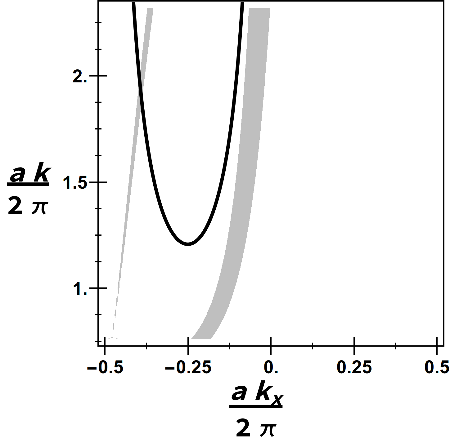
Figure 4: Comparison of the locations of the Dirac points given by the paraxial theory and a frequency-domain plane-wave simulation as $k$ is varied. In both cases Dirac points occur along the lines $k_{y}=0$ (top) and $k_{y}=\pi/a$ (bottom). Solid lines: $k_{x}$ for the Dirac points from the paraxial theory. Shading: bounds on $k_{x}$ for the Dirac points from the plane-wave simulations, where the magnitude of the splitting between the index surfaces is smaller than $a\Delta k_{z}=2\pi\times e^{-6}$. The dielectric parameters are those in Fig. 2. The plane-wave simulation has cylindrical air holes in the dielectric background, with a filling factor of $\pi(0.15)^{2}$.

In Fig. 4 we compare how the locations of the Dirac points evolve with the wavevector scale $k$, at fixed $a$, in the two theories. The solid black lines show the locations predicted by $H_{l}$, while those predicted numerically lie within the shaded regions of the figure. We see that $H_{l}$ gives a reasonable account of the numerical results. As shown in the upper panel, it correctly predicts the two Dirac points along the line $k_{y}=0$ for all values of $ka$, i.e., for all degrees of paraxiality. As expected there is a Dirac point along $k_{y}=0$ at $k_{x}=0$ in both theories. There is also a second Dirac point present in each theory along this line. For the periodic Hamiltonian model the second Dirac point is adjacent to the positive $k_{x}$ Brillouin zone boundary; for the the numerical simulations the Dirac point is found on the other side of this boundary displaced from the zone edge. We attribute this difference to the different treatment of scattering in the two methods, and perhaps also to higher-order terms neglected in Eq. (2). The lower panel of Fig. 4 shows the positions of Dirac points along the line $k_{y}=\pi/a$. While for small $ka$ the model $H_{l}$ lacks the two Dirac points seen in the numerical simulation, there is a critical $ka$ above which this additional pair emerges. Above this critical $ka$ the model $H_{l}$ is in qualitative agreement with the numerical simulation.

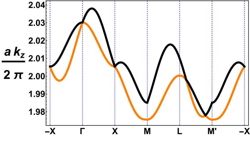
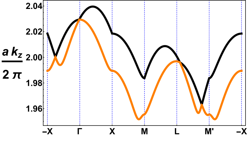
Figure 5: (Color online) Index surfaces along high-symmetry directions of the first Brillouin zone from the paraxial model (top panel) and a frequency-domain plane-wave calculation (lower panel). The relevant high-symmetry points are indicated in Fig. 2. $ka\simeq 4\pi$, and all other parameters are as in Figs. 2 and 4.

In Figure 5 we compare the index surfaces of the two theories, along a high-symmetry path through the Brillouin zone, for $ka\simeq 4\pi$. This degree of paraxiality places us in a regime towards the top of the vertical scale of the plots in Figure 4, in which there are four Dirac points in the Brillouin zone. As can be seen in this figure, there is a reasonable correspondence between the forms of the index surfaces of the two theories. As expected the shapes of the bands are somewhat different. Nonetheless, given the correspondence between the numbers and locations of the Dirac points across most degrees of paraxiality, the topological phase diagrams of the two models will be similar to one another. In the regime before the additional Dirac points emerge in the model $H_{l}$ the phase diagram of the numerical simulation will be richer than that of the model.

IV Discussion

In this paper we have explored the refractive index surfaces of two-dimensional photonic crystals. We have shown how optical activity can lead to photonic materials characterized by gapped, i.e. non-degenerate, index surfaces with non-zero Chern numbers. Our approach is unusual in that it does not rely on a specific lattice geometry, but instead on the conical intersections that occur generically in the index surface of optically anisotropic materials. This suggests that such topological photonic materials can be constructed with a range of lattice geometries.

For brevity we have referred to our material as a photonic Chern insulator. However, as can be seen from Fig. 5, it generally lacks a band gap at a particular propagation constant, and so is more accurately described as a photonic semi-metal with topological bands. In a true Chern insulator the topology of the bulk bands leads, in the presence of an interface, to the appearance of edge-states in the gap. For the semi-metal one does expect that a slow spatial variation of the structure from one topological phase to another will introduce modes crossing the bulk bands. However, a generic realistic interface would allow these modes to mix with the bulk bands and destroy their localization. Given that our proposal is not dependent on the particular form of lattice geometry, however, it should be possible to adapt the lattice to achieve a true Chern insulator. Furthermore, although one does not necessarily expect conventional edge states, topological semi-metals are known to have interesting properties in their own right Burkov (2016).

*

Appendix A Paraxial Hamiltonian

In this appendix we give the forms of the paraxial Hamiltonian $H_{p}$ for propagation close to the optic axis, in materials with biaxiality and anisotropic optical activity. They extend the results in Ref. Jeffrey, 2007 to include all terms up to second-order in the off-axis wavevectors, which is necessary to achieve a non-trivial topology for the periodic form of $H_{p}$. These expressions are obtained by rotating the spatial coordinates so that $z$ lies along an optic axis, expanding the expressions for $k_{z,\pm}$ to construct a diagonalized form for the paraxial Hamiltonian in the eigenbasis of $M$, and transforming the result out of this eigenbasis. For comparison with Ref. Berry et al., 2005 we use the scaled transverse wavevectors $p_{x,y}=k_{x,y}/k=\tilde{k}_{x,y}/\sqrt{\epsilon_{2}}$, where $k=k_{0}\sqrt{\epsilon_{2}}=\omega\sqrt{\epsilon_{2}}/c$ is the wavevector at frequency $\omega$ in an isotropic material of permittivity $\epsilon_{2}$. Note however that we use a circular polarization basis rather than the linear one of Ref. Berry et al., 2005.

Considering first a biaxial dielectric without optical activity, characterized by principal dielectric constants $\epsilon_{1}<\epsilon_{2}<\epsilon_{3}$, we find

$$\begin{split}h_{0,B}&=-Ap_{x}+\frac{1}{4}[2+\epsilon_{2}(\alpha-\beta)-12A^{2}]p_{x}^{2}+\\ &+\frac{1}{4}[2+\epsilon_{2}(\alpha-\beta)-6A^{2}]p_{y}^{2}.\\ h_{x,B}&=-Ap_{x}+\frac{1}{4}[\epsilon_{2}(\alpha-\beta)-12A^{2}]p_{x}^{2}\\ &\quad-\frac{1}{4}\epsilon_{2}(\alpha+3\beta)p_{y}^{2},\\ h_{y,B}&=-Ap_{y}+\frac{1}{2}[\epsilon_{2}(\alpha+\beta)-6A^{2}]p_{x}p_{y}.\\ h_{z,B}&=0.\end{split}$$ (5)

Here $\alpha=\epsilon_{1}^{-1}-\epsilon_{2}^{-1}$ and $\beta=\epsilon_{2}^{-1}-\epsilon_{3}^{-1}$ are measures of the spread of the principal dielectric constants of the biaxial material and $A$ is the biaxial cone semi-angle, defined as $A=\frac{1}{2}\epsilon_{2}\sqrt{\alpha\beta}$. Sufficiently close to the optic axis direction this Hamiltonian takes a Dirac point form.

Optical activity introduces an antisymmetric contribution to the inverse of the relative permittivity tensor $\eta_{ik}=(\epsilon^{-1})_{ik}$, corresponding to a contribution $\epsilon_{0}\bm{E}=i\bm{D}\times\bm{g}$ in the constitutive relation, where $\bm{g}$ is the optical activity vector Berry and Dennis (2003); Landau et al. (2008). In the case of the Faraday effect the optical activity vector is proportional to the applied field, $g_{i}=\gamma_{ij}H_{j}$, and independent of the wavevector. In the paraxial Hamiltonian this introduces additional terms in $h_{0}$, describing the field’s effect on the overall dispersion relation, as well as terms in $h_{3}$, describing the anisotropic splitting between the circular polarization states. The expressions for these components are

$$\begin{split}h_{0,F}&=h_{0,B}-\frac{3}{8}\epsilon_{2}^{2}\big{[}g^{\prime 2}_{3}+2g^{\prime}_{3}(g^{\prime}_{1}~{}p_{x}+g^{\prime}_{2}~{}p_{y})+\\ &+(g^{\prime 2}_{1}-g^{\prime 2}_{3})p_{x}^{2}+2g^{\prime}_{1}g^{\prime}_{2}~{}p_{x}p_{y}+(g^{\prime 2}_{2}-g^{\prime 2}_{3})p_{y}^{2}\big{]}.\end{split}$$ (6)

and

$$\begin{split}h_{z,F}&=\frac{1}{2}\epsilon_{2}\bigg{(}g^{\prime}_{3}+(g^{\prime}_{1}+3Ag^{\prime}_{3})p_{x}+g_{2}^{\prime}p_{y}\\ &\qquad\quad-\frac{1}{2}\{g^{\prime}_{3}[1+\frac{3}{2}\epsilon_{2}(\alpha-\beta)]-6Ag^{\prime}_{1}\}p_{x}^{2}\\ &\qquad\quad+3Ag^{\prime}_{2}p_{x}p_{y}-\frac{1}{2}\{g^{\prime}_{3}[1+\frac{3}{2}\epsilon_{2}(\alpha-\beta)]\}p_{y}^{2}\bigg{)}.\\ \end{split}$$ (7)

Here $\bm{g^{\prime}}$ is the optical activity vector in the rotated basis, where $z$ lies along the optic axis. The relation to the optical activity vector in the principal axes coordinate system (where $\epsilon$ is diagonal) is $\bm{g^{\prime}}=R\bm{g}$ with

$$R=\left(\begin{array}[]{ccc}\sqrt{\frac{\beta}{\alpha+\beta}}&0&-\sqrt{\frac{\alpha}{\alpha+\beta}}\\ 0&1&0\\ \sqrt{\frac{\alpha}{\alpha+\beta}}&0&\sqrt{\frac{\beta}{\alpha+\beta}}\end{array}\right).$$ (8)

For completeness we note that, in the case of a chiral medium, the optical activity vector is related to the wavevector direction, $g_{i}=\Gamma_{ij}\hat{k}_{j}$, by a symmetric tensor $\Gamma_{ij}$ Berry et al. (2005); Landau et al. (2008). This modifies the components $h_{0}$ and $h_{3}$ as follows:

$$\begin{split}h_{0,C}&=h_{0,B}-\frac{3}{8}\epsilon_{2}^{2}\big{\{}\Gamma^{\prime 2}_{33}+4\Gamma^{\prime}_{13}\Gamma^{\prime}_{33}p_{x}+4\Gamma^{\prime}_{23}\Gamma^{\prime}_{33}p_{y}+\\ &+[4\Gamma^{\prime 2}_{13}+2\Gamma^{\prime}_{33}(\Gamma^{\prime}_{11}-\Gamma^{\prime}_{33})]p_{x}^{2}+\\ &+4(\Gamma^{\prime}_{12}\Gamma^{\prime}_{33}+2\Gamma^{\prime}_{13}\Gamma^{\prime}_{23})p_{x}p_{y}+\\ &+[4\Gamma^{\prime 2}_{23}+2\Gamma^{\prime}_{33}(\Gamma^{\prime}_{22}-\Gamma^{\prime}_{33})]p_{y}^{2}\big{\}}.\end{split}$$ (9)

and

$$\begin{split}h_{z,C}&=\frac{1}{2}\epsilon_{2}\bigg{(}\Gamma^{\prime}_{33}+(2\Gamma^{\prime}_{13}+3A\Gamma^{\prime}_{33})~{}p_{x}+2\Gamma^{\prime}_{23}~{}p_{y}\\ &\qquad\qquad+\{\Gamma^{\prime}_{11}+6A\Gamma^{\prime}_{13}-[1+\frac{3}{4}\epsilon_{2}(\alpha-\beta)]\Gamma^{\prime}_{33}\}p_{x}^{2}\\ &\qquad\qquad+(2\Gamma^{\prime}_{12}+6A\Gamma^{\prime}_{23})~{}p_{x}p_{y}\\ &\qquad\qquad+\{\Gamma^{\prime}_{22}-[1+\frac{3}{4}\epsilon_{2}(\alpha-\beta)]\Gamma^{\prime}_{33}\}p_{y}^{2}\bigg{)}.\\ \end{split}$$ (10)

where the tensor $\Gamma^{\prime}$ is related to the corresponding tensor in the principal axes basis by $\Gamma^{\prime}=R\Gamma R^{-1}$.

References

- Klitzing et al. (1980) K. v. Klitzing, G. Dorda, and M. Pepper, Phys. Rev. Lett. 45, 494 (1980).
- Avron et al. (1983) J. E. Avron, R. Seiler, and B. Simon, Phys. Rev. Lett. 51, 51 (1983).
- Kohmoto (1985) M. Kohmoto, Ann. Phys. (NY) 160, 343 (1985).
- Thouless et al. (1982) D. J. Thouless, M. Kohmoto, M. P. Nightingale, and M. den Nijs, Phys. Rev. Lett. 49, 405 (1982).
- Hatsugai (1993) Y. Hatsugai, Phys. Rev. Lett. 71, 3697 (1993).
- Haldane (1988) F. D. M. Haldane, Phys. Rev. Lett. 61, 2015 (1988).
- Sticlet et al. (2012) D. Sticlet, F. Piéchon, J.-N. Fuchs, P. Kalugin, and P. Simon, Phys. Rev. B 85, 165456 (2012).
- Raghu and Haldane (2008) S. Raghu and F. D. M. Haldane, Phys. Rev. A 78, 033834 (2008).
- Haldane and Raghu (2008) F. D. M. Haldane and S. Raghu, Phys. Rev. Lett. 100, 013904 (2008).
- Ochiai and Onoda (2009) T. Ochiai and M. Onoda, Phys. Rev. B 80, 155103 (2009).
- Wang et al. (2008) Z. Wang, Y. D. Chong, J. D. Joannopoulos, and M. Soljačić, Phys. Rev. Lett. 100, 013905 (2008).
- Wang et al. (2009) Z. Wang, Y. Chong, J. D. Joannopoulos, and M. Soljacic, Nature 461, 772 (2009).
- Rechtsman et al. (2013) M. C. Rechtsman, J. M. Zeuner, Y. Plotnik, Y. Lumer, D. Podolsky, F. Dreisow, S. Nolte, M. Segev, and A. Szameit, Nature 496, 196 (2013).
- Poo et al. (2011) Y. Poo, R.-x. Wu, Z. Lin, Y. Yang, and C. T. Chan, Phys. Rev. Lett. 106, 093903 (2011).
- Khanikaev et al. (2013) A. B. Khanikaev, S. Hossein Mousavi, W.-K. Tse, M. Kargarian, A. H. MacDonald, and G. Shvets, Nat Mater 12, 233 (2013).
- Chen et al. (2014) W.-J. Chen, S.-J. Jiang, X.-D. Chen, B. Zhu, L. Zhou, J.-W. Dong, and C. T. Chan, Nat. Commun. 5, 5782 (2014).
- Ma et al. (2015) T. Ma, A. B. Khanikaev, S. H. Mousavi, and G. Shvets, Phys. Rev. Lett. 114, 127401 (2015).
- Slobozhanyuk et al. (2017) A. Slobozhanyuk, H. S. Mousavi, X. Ni, D. Smirnova, Y. S. Kivshar, and A. B. Khanikaev, Nat. Photon 11, 130 (2017).
- Bardyn et al. (2015) C.-E. Bardyn, T. Karzig, G. Refael, and T. C. H. Liew, Phys. Rev. B 91, 161413 (2015).
- Nalitov et al. (2015) A. V. Nalitov, D. D. Solnyshkov, and G. Malpuech, Phys. Rev. Lett. 114, 116401 (2015).
- Karzig et al. (2015) T. Karzig, C.-E. Bardyn, N. H. Lindner, and G. Refael, Phys. Rev. X 5, 031001 (2015).
- Yi and Karzig (2016) K. Yi and T. Karzig, Phys. Rev. B 93, 104303 (2016).
- Prodan and Prodan (2009) E. Prodan and C. Prodan, Phys. Rev. Lett. 103, 248101 (2009).
- Kane and Lubensky (2014) C. L. Kane and T. C. Lubensky, Nat. Phys. 10, 39 (2014).
- Yang et al. (2015) Z. Yang, F. Gao, X. Shi, X. Lin, Z. Gao, Y. Chong, and B. Zhang, Phys. Rev. Lett. 114, 114301 (2015).
- Gao et al. (2015) W. Gao, M. Lawrence, B. Yang, F. Liu, F. Fang, B. Béri, J. Li, and S. Zhang, Phys. Rev. Lett. 114, 037402 (2015).
- Berry and Jeffrey (2006) M. V. Berry and M. R. Jeffrey, J. Opt. A 8, 363 (2006).
- Born and Wolf (1999) M. Born and E. Wolf, Principles of Optics, 7th ed. (CUP, 1999).
- Landau et al. (2008) L. D. Landau, E. M. Lifshitz, and L. P. Pitaevskii, Electrodynamics of continuous media, 2nd ed., Course of theoretical physics (Elsevier, Butterworth-Heinemann, Amsterdam, 2008).
- Berry et al. (2006) M. Berry, M. Jeffrey, and J. Lunney, Proc. Royal Soc. Lond. A 462, 1629 (2006).
- Berry and Dennis (2003) M. V. Berry and M. R. Dennis, Proc. Royal Soc. Lond. A 459, 1261 (2003).
- Berry (2004) M. V. Berry, J. Opt. A 6, 289 (2004).
- Jeffrey (2007) M. Jeffrey, Conical Diffraction: Complexifying Hamilton’s Diabolical Legacy, Ph.D. thesis, University of Bristol (2007).
- Fukui et al. (2005) T. Fukui, Y. Hatsugai, and H. Suzuki, J. Phys. Soc. Jpn. 74, 1674 (2005).
- Johnson and Joannopoulos (2001) S. G. Johnson and J. D. Joannopoulos, Opt. Express 8, 173 (2001).
- Burkov (2016) A. Burkov, Nat. Mater. 15, 1145 (2016).
- Berry et al. (2005) M. V. Berry, M. R. Jeffrey, and M. Mansuripur, J. Opt. A 7, 685 (2005).