A mixed finite element method for nearly incompressible multiple-network poroelasticity

Abstract

In this paper, we present and analyze a new mixed finite element formulation of a general family of quasi-static multiple-network poroelasticity (MPET) equations. The MPET equations describe flow and deformation in an elastic porous medium that is permeated by multiple fluid networks of differing characteristics. As such, the MPET equations represent a generalization of Biot’s equations, and numerical discretizations of the MPET equations face similar challenges. Here, we focus on the nearly incompressible case for which standard mixed finite element discretizations of the MPET equations perform poorly. Instead, we propose a new mixed finite element formulation based on introducing an additional total pressure variable. By presenting energy estimates for the continuous solutions and a priori error estimates for a family of compatible semi-discretizations, we show that this formulation is robust in the limits of incompressibility, vanishing storage coefficients, and vanishing transfer between networks. These theoretical results are corroborated by numerical experiments. Our primary interest in the MPET equations stems from the use of these equations in modelling interactions between biological fluids and tissues in physiological settings. So, we additionally present physiologically realistic numerical results for blood and tissue fluid flow interactions in the human brain.

65M12, 65M15, 65M60, 92C10

1 Introduction

In this paper, we consider a family of quasi-static multiple-network poroelasticity (MPET) equations reading as follows: for a given number of networks $A\in\mathbb{N}$, find the displacement $u$ and the network pressures $p_{j}$ for $j=1,\dots,A$ such that

(1.1a) $$-\operatorname{div}C\varepsilon(u)+\operatorname{\textstyle\sum}_{j}\alpha_{j}\operatorname{\nabla}p_{j} =f,$$

(1.1b) $$c_{j}\dot{p}_{j}+\alpha_{j}\operatorname{div}\dot{u}-\operatorname{div}K_{j}\operatorname{\nabla}p_{j}+S_{j} =g_{j},\qquad 1\leq j\leq A,$$

where $u=u(x,t)$ and $p_{j}=p_{j}(x,t)$, $1\leq j\leq A$ for $x\in\Omega\subset{\mathbb{R}}^{d}$ ($d=1,2,3$) and for $t\in[0,T]$.

In our context, (1.1) originates from balance of mass and momentum in a porous, linearly elastic medium permeated by $A$ segregated viscous fluid networks. The operators and parameters are as follows: $C$ is the elastic stiffness tensor, each network $j$ is associated with a Biot-Willis coefficient $\alpha_{j}\in(0,1]$, storage coefficient $c_{j}\geq 0$, and hydraulic conductivity tensor $K_{j}=\kappa_{j}/\mu_{j}>0$ (where $\kappa_{j}$ and $\mu_{j}$ represent the network permeability and the network fluid viscosity, respectively). In (1.1a), $\operatorname{\nabla}$ denotes the gradient, $\varepsilon$ is the symmetric (row-wise) gradient, $\operatorname{div}$ denotes the row-wise divergence. In (1.1b), $\operatorname{\nabla}$ and $\operatorname{div}$ are the standard gradient and divergence operators, and the superposed dot denotes the time derivative. Further, $f$ represents a body force and $g_{j}$ represents sources in network $j$ for $j=1,\dots,A$, while $S_{j}$ represents transfer terms out of network $j$.

In this paper, we consider the case of an isotropic stiffness tensor for which

(1.2) $$C\varepsilon(u)=2\mu\varepsilon(u)+\lambda\operatorname{div}uI$$

where $\mu,\lambda$ are the standard non-negative Lamé parameters and $I$ denotes the identity tensor. Moreover, we will consider the case where the transfer terms $S_{j}$, quantifying the transfer out of network $j$ into the other fluid networks, are proportional to pressure differences between the networks. More precisely, we assume that $S_{j}$ takes the form:

(1.3) $$S_{j}=S_{j}(p_{1},\dots,p_{A})=\operatorname{\textstyle\sum}_{i=1}^{A}\xi_{j\leftarrow i}(p_{j}-p_{i}),$$

where $\xi_{j\leftarrow i}$ are non-negative transfer coefficients for $i,j=1,\dots,A$. We will also assume that these transfer coefficients are symmetric in the sense that $\xi_{j\leftarrow i}=\xi_{i\leftarrow j}$, and note that $\xi_{j\leftarrow j}$ is arbitrary.

The MPET equations have an abundance of both geophysical and biological applications. In the case $A=1$, (1.1) reduces to the well-known quasi-static Biot equations. While the Biot equations have been studied extensively, see e.g. [32, 25, 29, 2, 28, 22, 38]; to the best of our knowledge, the general multiple-network poroelasticity equations have received much less attention, especially from the numerical perspective. The case $A=2$ is known as the Barenblatt-Biot model, and we note that Showalter and Momken [33] present an existence analysis for this model, while Nordbotten and co-authors [27] present an a posteriori error analysis for an approximation of a static Barenblatt-Biot system.

Our interest in the multiple-network poroelasticity equations primarily stems from the use of these equations in modelling interactions between biological fluids and tissue in physiological settings. As one example, Tully and Ventikos [35] considers (1.1) with four different networks ($A=4$) to model fluid flows, network pressures and elastic displacement in brain tissue. The fluid networks represent the arteries, the arterioles/capillaries, the veins and the interstitial fluid-filled extracellular space, each network with e.g. a different permeability $\kappa_{j}$ and different transfer coefficients $\xi_{j\leftarrow i}$.

A particularly important motivation for the current work is the recently proposed theory of the glymphatic system which describes a new mechanism for waste clearance in the human brain [18, 19, 1]. This mechanism is proposed to take the form of a convective flow of water-like fluid through (a) spaces surrounding the cerebral vasculature (paravascular spaces) and (b) through the extracellular spaces, driven by a hydrostatic pressure gradient between the arterial and venous compartments. Compared to diffusion only, such a convective flow would lead to enhanced transport of solutes through the brain parenchyma and, in particular, contribute to clearance of metabolic waste products such as amyloid beta. The accumulation of amyloid beta frequently seen in patients with Alzheimer’s disease is as such seen as a malfunction of the glymphatic system. In this context, the original system of [35] represents a macroscopic model of interaction between the different fluid networks in the brain.

Discretization of Biot’s equations is known to be challenging, in particular because of so-called poroelastic locking. Poroelastic locking has two main characteristics: 1) underestimation of the solid deformation if the material is close to being incompressible and 2) nonphysical pressure oscillations, in particular in the areas close to jumps in the permeabilities or to the boundary. Several recent (and not so recent) studies, see e.g. [29, 6, 4, 17, 31, 38], focus on a three-field formulation of Biot’s model, involving the elastic displacement, fluid pressure and fluid velocity. Four-field formulations where also the elasticity equation is in mixed form, designed to provide robust numerical methods for nearly incompressible materials, have also been studied [37, 20, 21].

In biological tissues, any jumps in the permeability parameters are typically small in contrast to geophysical applications. The challenge in the biomedical applications is rather that the tissues in our body mostly consist of water and as such should be close to be incompressible (for short time-scales and normal physiological pressures). Therefore, it may be crucial for accurate modeling of the interaction of the different network pressures in (1.1) to allow for an elastic material that is almost incompressible and/or with (nearly) vanishing storage coefficients, i.e. for $1\ll\lambda<+\infty$ and $0<c_{j}\ll 1$ in (1.1). Standard two-field mixed finite element discretizations of the Biot model, approximating the displacement and the fluid pressure only using Stokes-stable elements, are well-known to perform poorly in the incompressible limit, see e.g. [22] and references therein. Moreover, we can easily demonstrate a suboptimal convergence rate for the corresponding standard mixed finite element discretization of the MPET equations, see Example 1 below. On the other hand, two-field approximations are computationally inexpensive compared to three-field approximations in the sense that only one unknown, the network pressure, is involved in each network.

Example .

To illustrate poor performance of a standard mixed finite element discretization of the MPET equations (1.1) in the nearly incompressible case, we consider a variant of the smooth test case presented by [38, Section 7.1]. Let $\Omega=[0,1]^{2}\subset{\mathbb{R}}^{2}$, take $T=0.5$, and consider the quasi-static multiple-network poroelasticity equations (1.1) with $A=2$, $c_{j}=1.0$, $K_{j}=1.0$, $\alpha_{j}=1.0$, and $S_{j}=0$ for $j=1,2$. Moreover, we let $E=1.0$ and $\nu=0.49999$ for

$$\mu=\frac{E}{2(1+\nu)}\approx\frac{1}{3},\quad\lambda=\frac{\nu E}{(1-2\nu)(1+\nu)}\approx 16\,666.$$

To discretize (1.1), we consider a Crank-Nicolson discretization in time and a standard mixed finite element discretization in space in this example. More precisely, we approximate the displacement $u$ using continuous piecewise quadratic vector fields (and denote the approximation by $u_{h}$) and the fluid pressures $p_{j}$ for $j=1,2$ using continuous piecewise linears defined relative to a uniform mesh of $\Omega$ of mesh size $h$. As exact solutions, we let

$$u((x_{0},x_{1}),t)=t\begin{pmatrix}(\sin(2\pi x_{1})(-1+\cos(2\pi x_{0}))+\frac{1}{\mu+\lambda}\sin(\pi x_{0})\sin(\pi x_{1}))\\ (\sin(2\pi x_{0})(1-\cos(2\pi x_{1}))+\frac{1}{\mu+\lambda}\sin(\pi x_{0})\sin(\pi x_{1}))\end{pmatrix},$$

and

$$p_{j}((x_{0},x_{1},t))=-jt\sin(\pi x_{0})\sin(\pi x_{1}).$$

The resulting approximation errors for $u(T)$ in the $L^{2}(\Omega)$ and $H^{1}(\Omega)$ norms are listed in Table 1 for a series of meshes generated by nested uniform refinements, together with the corresponding rates of convergence. We observe that the convergence rates are one order sub-optimal for this choice of spatial discretization.

$h$	$\|u(T)-u_{h}(T)\|$	Rate	$\|u(T)-u_{h}(T)\|_{H^{1}}$	Rate
$H$	0.169		2.066
$H/2$	0.040	2.09	0.980	1.08
$H/4$	0.010	2.04	0.480	1.03
$H/8$	0.002	2.03	0.235	1.03
$H/16$	0.001	2.09	0.110	1.10
Optimal		3		2

Table 1: Approximation errors in the $L^{2}$ ($\|\cdot\|$)- and $H^{1}$ ($\|\cdot\|_{H^{1}}$)-norms and associated convergence rates for a standard mixed finite element discretization for a smooth manufactured solution test case for a nearly incompressible material (Example 1). $H$ corresponds to a uniform mesh constructed by dividing the unit square into $4\times 4$ squares and dividing each square by a diagonal.

The primary objective of this paper is to propose and analyze a new variational formulation and a corresponding spatial discretization of the MPET equations that are robust with respect to a nearly incompressible poroelastic matrix; i.e. the implicit constants in the error estimates are uniformly bounded for arbitrarily large $\lambda>0$. To this end, we introduce a formulation with one additional scalar field unknown. For the MPET equations (1.1) with potentially multiple networks, the additional computational cost is thus small. Instead of taking the ”solid pressure” $\lambda\operatorname{div}u$ as a new unknown, we take the total pressure, which is defined as a weighted sum of the network pressures and the solid pressure, as the new unknown. Such a formulation has previously been shown to be advantageous in the context of parameter-robust preconditioners for the Biot model [23]. Here, we focus on stability and error estimates of the total pressure formulation for the more general MPET equations. The construction of preconditioners for the MPET equations will be addressed in a forthcoming paper.

Our new theoretical results include an energy estimate for the continuous variational formulation that is robust in the relevant parameter limits, in particular, that is uniform in the Lamé parameter $\lambda$, storage coefficients $c_{j}$ for $j=1,\dots,A$, and transfer coefficients $\xi_{j\leftarrow i}$ for $i,j=1,\dots,A$, and a robust a priori error estimate for a class of compatible semi-discretizations of the new formulation. These theoretical results are supported by numerical experiments. Finally, we also present new numerical MPET simulations modelling blood and tissue fluid interactions in a physiologically realistic human brain.

This paper is organized as follows. Section 2 presents notation and general preliminaries. In Section 3, we introduce a total-pressure-based variational formulation (3.6) for the quasi-static MPET equations (1.1), together with a robust energy estimate in Theorem 3.3. We continue in Section 4 by proposing a general class of compatible semi-discretizations (4.1) of this formulation, and estimate the a priori discretization errors in Proposition 1 and the semi-discrete errors for a specific choice of finite element spaces in Theorem 4.2 and Proposition 2. These theoretical results are corroborated by synthetic numerical convergence experiments in Section 5. In Section 6, we present a more physiologically realistic numerical experiment using a 4-network MPET model to investigate blood and tissue fluid flow in the human brain. Some conclusions and directions of future research are highlighted in Section 7.

2 Notation and preliminaries

Throughout this paper we use $X\lesssim Y$ to denote the inequality $X\leq CY$ with a generic constant $C>0$ which is independent of mesh sizes. If needed, we will write $C$ explicitly in inequalities but it can vary across expressions.

2.1 Sobolev spaces

Let $\Omega$ be a bounded polyhedral domain in ${\mathbb{R}}^{d}$ ($d=1,2$, or $3$) with boundary $\partial\Omega$. We let $L^{2}(\Omega)$ be the set of square-integrable real-valued functions on $\Omega$. The inner product of $L^{2}(\Omega)$ and the induced norm are denoted by $\langle\cdot,\cdot\rangle$ and $\|\cdot\|$, respectively. For a finite-dimensional inner product space ${\mathbb{X}}$, typically ${\mathbb{X}}={\mathbb{R}}^{d}$, let $L^{2}(\Omega;{\mathbb{X}})$ be the space of ${\mathbb{X}}$-valued functions such that each component is in $L^{2}(\Omega)$. The inner product of $L^{2}(\Omega;{\mathbb{X}})$ is naturally defined by the inner product of ${\mathbb{X}}$ and $L^{2}(\Omega)$, so we use the same notation $\langle\cdot,\cdot\rangle$ and $\|\cdot\|$ to denote the inner product and norm on $L^{2}(\Omega;{\mathbb{X}})$. For a non-negative real-valued function on $\Omega$ (or symmetric positive semi-definite tensor-valued function on $\Omega$) $w$, we also introduce the short-hand notations

(2.1) $$\langle u,v\rangle_{w}=\langle wu,v\rangle,\quad\|u\|_{w}^{2}=\langle u,u\rangle_{w},$$

noting that the latter is a norm only when $w$ is strictly positive a.e. on $\Omega$ (or is positive definite a.e. on $\Omega$).

For a non-negative integer $m$, $H^{m}(\Omega)$ denotes the standard Sobolev spaces of real-valued functions based on the $L^{2}$-norm, and $H^{m}(\Omega;{\mathbb{X}})$ is defined similarly based on $L^{2}(\Omega;{\mathbb{X}})$. To avoid confusion with the weighted $L^{2}$-norms cf. (2.1) we use $\|\cdot\|_{H^{m}}$ to denote the $H^{m}$-norm (both for $H^{m}(\Omega)$ and $H^{m}(\Omega;{\mathbb{X}})$). For $m\geq 1$, we use $H^{m}_{0,\Gamma}(\Omega)$ to denote the subspace of $H^{m}(\Omega)$ with vanishing trace on $\Gamma\subset\partial\Omega$, and $H^{m}_{0,\Gamma}(\Omega;{\mathbb{X}})$ is defined similarly [14]. For $\Gamma=\partial\Omega$, we write $H^{m}_{0}(\Omega)$ and analogously $H^{m}_{0}(\Omega;{\mathbb{X}})$.

2.2 Spaces involving time

We will consider an interval $[0,T]$, $T>0$. For a reflexive Banach space $\mathcal{X}$, let $C^{0}([0,T];\mathcal{X})$ denote the set of functions $f:[0,T]\rightarrow\mathcal{X}$ that are continuous in $t\in[0,T]$. For an integer $m\geq 1$, we define

$$C^{m}([0,T];\mathcal{X})=\{f\,|\,\partial^{i}f/\partial t^{i}\in C^{0}([0,T];\mathcal{X}),\,0\leq i\leq m\},$$

where $\partial^{i}f/\partial t^{i}$ is the $i$-th time derivative in the sense of the Fréchet derivative in $\mathcal{X}$ (see e.g. [39]).

For a function $f:[0,T]\rightarrow\mathcal{X}$, we define the space-time norm

$$\|f\|_{L^{r}([0,T];\mathcal{X})}=\begin{cases}\left(\int_{0}^{T}\|f(s)\|_{\mathcal{X}}^{r}\,\mathrm{d}s\right)^{1/r},\quad 1\leq r<\infty,\\ \operatorname{ess\,sup}_{t\in[0,T]}\|f(t)\|_{\mathcal{X}},\quad r=\infty.\end{cases}$$

We define the space-time Sobolev spaces $W^{k,r}([0,T];\mathcal{X})$ for a non-negative integer $k$ and $1\leq r\leq\infty$ as the closure of $C^{k}([0,T];\mathcal{X})$ with the norm $\|f\|_{W^{k,r}([0,T];\mathcal{X})}=\sum_{i=0}^{k}\|\partial^{i}f/\partial t^{i}\|_{L^{r}([0,T];\mathcal{X})}$.

2.3 Finite element spaces

Let $\mathcal{T}_{h}$ be an admissible, conforming, simplicial tessellation of the domain $\Omega$. For any integer $k\geq 1$, we let $\mathcal{P}_{k}(\mathcal{T}_{h})$ denote the space of continuous piecewise polynomials of order $k$ defined relative to $\mathcal{T}_{h}$, and $\mathcal{P}_{k}^{d}(\mathcal{T}_{h})$ as the space of $d$-tuples with components in $\mathcal{P}_{k}$. We will typically omit the reference to $\mathcal{T}_{h}$ when context allows. We let $\mathring{\mathcal{P}_{k}}$ denote the restriction of these piecewise polynomial spaces to conform with given essential homogeneous boundary conditions.

2.4 Parameter values

Based on physical considerations and typical applications, we will make the following assumptions on the material parameter values. First, we assume that the Biot-Willis coefficients $\alpha_{j}\in(0,1]$, $j=1,\dots,A$, and the storage coefficients $c_{j}>0$ are constant in time for $j=1,\dots,A$. In the analysis, we will pay particular attention to robustness of estimates with respect to arbitrarily large $\lambda$ and arbitrarily small (but not vanishing) $c_{j}$’s. We also comment on the case $c_{j}=0$ in Remark 4.4.

We will assume that the hydraulic conductivities $K_{j}$ are constant in time, but possibly spatially-varying and that these satisfy standard ellipticity constraints: i.e. there exist positive constants $K_{j}^{-}$ and $K_{j}^{+}$ such that

$$K_{j}^{-}\leq K_{j}(x)\leq K_{j}^{+}\quad\forall\,x\in\Omega.$$

We assume that the transfer coefficients $\xi_{j\leftarrow i}$ are constant in time and non-negative: i.e. $\xi_{j\leftarrow i}(x)\geq 0$ for $1\leq i,j\leq A$, $x\in\Omega$.

2.5 Boundary conditions

We will consider (1.1) augmented by the following standard boundary conditions. First, we assume that the boundary decomposes in two parts: $\partial\Omega=\Gamma_{D}\cup\Gamma_{N}$ with $\Gamma_{D}\cap\Gamma_{N}=\emptyset$ and $|\Gamma_{D}|,|\Gamma_{N}|>0$ where $|\Gamma|$ is the Lebesgue measure of $\Gamma$. We use $n$ to denote the outward unit normal vector field on $\partial\Omega$. Relative to this partition, we consider the homogeneous boundary conditions

(2.2a) $$u =0\quad\text{ on }\Gamma_{D},$$

(2.2b) $$C\varepsilon(u)\cdot n =0\quad\text{ on }\Gamma_{N},$$

(2.2c) $$p_{j} =0\quad\text{ on }\partial\Omega\quad\text{ for }j=1,\dots,A.$$

The subsequent formulation and analysis can easily be extended to cover inhomogeneous and other types of boundary conditions.

2.6 Key inequalities

For the space $V=H^{1}_{0,\Gamma_{D}}(\Omega)$, Korn’s inequality [9, p. 288] holds; i.e. there exists a constant $C>0$ depending only on $\Omega$ and $\Gamma_{D}$ such that

(2.3) $$\|u\|\leq C\|\varepsilon(u)\|\quad\forall\,u\in V.$$

Furthermore, for the combination of spaces $V$ and $Q_{0}=L^{2}(\Omega)$, the following (continuous Stokes) inf-sup condition holds: there exists a constant $C>0$ depending only on $\Omega$ and $\Gamma_{D}$ such that

(2.4) $$\sup_{u\in V}\frac{\langle\operatorname{div}u,q\rangle}{\|u\|_{H^{1}}}\geq C\|q\|\quad\forall\,q\in L^{2}(\Omega).$$

Our discretization schemes will also satisfy corresponding discrete versions of Korn’s inequality and the inf-sup condition with constants independent of the discretization.

2.7 Initial conditions

The MPET equations (1.1) must also be complemented by appropriate initial conditions. In particular, in agreement with the assumption that $c_{j}>0$ for $j=1,\dots,A$, we assume that initial conditions are given for all $p_{j}$:

(2.5) $$p_{j}(x,0)=p_{j}^{0}(x),\quad x\in\Omega,\quad j=1,\dots,A.$$

Given such $p_{j}^{0}$, we note that we may compute $u(x,0)=u^{0}(x)$ from (1.1a), which in particular yields a $\operatorname{div}u(x,0)=\operatorname{div}u^{0}(x)$ for $x\in\Omega$. In the following, we will assume that any initial conditions given are compatible in the sense described here.

3 A new formulation for multiple-network poroelasticity

In this section, we introduce a new variational formulation for the quasi-static multiple-network poroelasticity equations targeting the incompressible and nearly incompressible regime. Inspired by [28, 23], we introduce an additional variable, namely the total pressure. In the subsequent subsections, we present the augmented governing equations, introduce a corresponding variational formulation, and demonstrate the robustness of this formulation via an energy estimate.

3.1 Governing equations introducing the total pressure

Let $u$ and $p_{j}$ for $j=1,\dots,A$ be solutions of (1.1) with boundary conditions given by (2.2), initial conditions given by (2.5) and recall the isotropic stiffness tensor assumption, cf. (1.2). Additionally, we now introduce the total pressure $p_{0}$ defined as

(3.1) $$p_{0}=\lambda\operatorname{div}u-\operatorname{\textstyle\sum}_{j=1}^{A}\alpha_{j}p_{j}.$$

Defining $\alpha_{0}=1$ for the purpose of short-hand, and rearranging, we thus have that

(3.2) $$\operatorname{div}u=\lambda^{-1}\operatorname{\textstyle\sum}_{i=0}^{A}\alpha_{i}p_{i}.$$

For simplicity, we denote $\alpha=(\alpha_{0},\alpha_{1},\dots,\alpha_{A})$ and $p=(p_{0},p_{1},\dots,p_{A})$, and we can thus write

$$\operatorname{\textstyle\sum}_{i=0}^{A}\alpha_{i}p_{i}=\alpha\cdot p$$

in the following.

Inserting (3.2) and its time-derivative into (1.1b), we obtain an augmented system of quasi-static multiple-network poroelasticity equations: for $t\in(0,T]$, find the displacement vector field $u$ and the pressure scalar fields $p_{i}$ for $i=0,\dots,A$ such that

(3.3a) $$\operatorname{div}u-\lambda^{-1}\alpha\cdot p =0,$$

(3.3b) $$-\operatorname{div}\left(2\mu\varepsilon(u)+p_{0}I\right) =f,$$

(3.3c) $$c_{j}\dot{p}_{j}+\alpha_{j}\lambda^{-1}\alpha\cdot\dot{p}-\operatorname{div}(K_{j}\nabla p_{j})+S_{j} =g_{j}\quad j=1,\dots,A.$$

We note that $p_{0}(x,0)$ can be computed from (2.5) and (3.1).

Remark .

In the limit $\lambda=\infty$, the equations for the displacement $u$ and total pressure $p_{0}$, and the network pressures $p_{i}$ decouple, and (3.3) reduces to a Stokes system for $(u,p_{0})$ and a system of parabolic equations for $p_{j}$:

$$-\operatorname{div}\left(2\mu\varepsilon(u)+p_{0}I\right) =f,$$

$$\operatorname{div}u =0,$$

$$c_{j}\dot{p}_{j}-\operatorname{div}(K_{j}\nabla p_{j})+S_{j} =g_{j}\quad j=1,\dots,A.$$

We next present and study a continuous variational formulation based on the total pressure formulation (3.3) of the quasi-static multiple-network poroelasticity equations.

3.2 Variational formulation

With reference to the notation for domains and Sobolev spaces as introduced in Section 2, let

(3.5) $$V=H^{1}_{0,\Gamma_{D}}(\Omega;{\mathbb{R}}^{d}),\quad Q_{0}=L^{2}(\Omega),\quad Q_{j}=H^{1}_{0}(\Omega)\quad j=1,\dots,A.$$

Also denote $Q=Q_{0}\times Q_{1}\times\dots\times Q_{A}$.

Multiplying (3.3) by test functions and integrating by parts with boundary conditions given by (2.2) and initial conditions given by (2.5) yield the following variational formulation: given compatible $u^{0}$ and $p_{j}^{0}$, $f$ and $g_{j}$ for $j=1,\dots,A$, find $u\in C^{1}([0,T];V)$ and $p_{i}\in C^{1}([0,T],Q_{i})$ for $i=0,\dots,A$ such that

(3.6a) $$\langle 2\mu\varepsilon(u),\varepsilon(v)\rangle+\langle p_{0},\operatorname{div}v\rangle =\langle f,v\rangle \quad\forall\,v\in V,$$

(3.6b) $$\langle\operatorname{div}u,q_{0}\rangle-\langle\lambda^{-1}\alpha\cdot p,q_{0}\rangle =0 \quad\forall\,q_{0}\in Q_{0},$$

(3.6c) $$\langle c_{j}\dot{p}_{j}+\alpha_{j}\lambda^{-1}\alpha\cdot\dot{p}+S_{j},q_{j}\rangle+\langle K_{j}\operatorname{\nabla}p_{j},\operatorname{\nabla}q_{j}\rangle =\langle g_{j},q_{j}\rangle \quad\forall\,q_{j}\in Q_{j},$$

for $j=1,\dots,A$ and such that $u(\cdot,0)=u^{0}(\cdot)$ and $p_{j}(\cdot,0)=p_{j}^{0}(\cdot)$ for $j=1,\dots,A$.

The following lemma is a modified version of Lemma 3.1 in [21] and will be used in the energy estimates below. For the sake of completeness, we present its proof here.

Lemma 3.1.

Let $\mathcal{F}$, $\mathcal{G}$, $\mathcal{G}_{1}$, $\mathcal{X}:[0,T]\rightarrow{\mathbb{R}}$ be continuous, non-negative functions. Suppose that $\mathcal{X}(t)$ satisfies

(3.7) $$\mathcal{X}^{2}(t)\leq C_{0}\mathcal{X}^{2}(0)+C_{1}\mathcal{X}(0)+\mathcal{G}_{1}(t)+\int_{0}^{t}\left[\mathcal{F}(s)\mathcal{X}(s)+\mathcal{G}(s)\right]\,\mathrm{d}s,$$

for all $t\in[0,T]$ with constants $C_{0}\geq 1$ and $C_{1}>0$. Then for any $t\in[0,T]$,

(3.8) $$\mathcal{X}(t)\lesssim\mathcal{X}(0)+\max\left\{C_{1}+\int_{0}^{t}\mathcal{F}(s)\,\mathrm{d}s,\left(\mathcal{G}_{1}(t)+\int_{0}^{t}\mathcal{G}(s)\,\mathrm{d}s\right)^{\frac{1}{2}}\right\}.$$

Proof 3.2.

It suffices to show the estimate for the smallest $t$ such that

$$\mathcal{X}(t)=\max_{s\in[0,T]}\mathcal{X}(s).$$

By this assumption, $\mathcal{X}(t)=\max_{s\in[0,T]}\mathcal{X}(s)$ and $\mathcal{X}(s)<\mathcal{X}(t)$ for all $0\leq s<t$. We now consider two cases: either

(3.9) $$C_{1}\mathcal{X}(0)+\int_{0}^{t}\mathcal{F}(s)\mathcal{X}(s)\,\mathrm{d}s\geq\mathcal{G}_{1}(t)+\int_{0}^{t}\mathcal{G}(s)\,\mathrm{d}s$$

or

(3.10) $$C_{1}\mathcal{X}(0)+\int_{0}^{t}\mathcal{F}(s)\mathcal{X}(s)\,\mathrm{d}s<\mathcal{G}_{1}(t)+\int_{0}^{t}\mathcal{G}(s)\,\mathrm{d}s.$$

If (3.9) holds, then (3.7) gives

$$\mathcal{X}^{2}(t) \leq C_{0}\mathcal{X}^{2}(0)+2C_{1}\mathcal{X}(0)+2\int_{0}^{t}\mathcal{F}(s)\mathcal{X}(s)\,\mathrm{d}s$$

$$\leq C_{0}\mathcal{X}^{2}(0)+2C_{1}\mathcal{X}(0)+2\mathcal{X}(t)\int_{0}^{t}\mathcal{F}(s)\,\mathrm{d}s.$$

Dividing both sides by $\mathcal{X}(t)$ yields (3.8) because $\mathcal{X}(t)\geq\mathcal{X}(0)$.

On the other hand, if (3.10) is the case, then (3.7) gives

$$\mathcal{X}^{2}(t) \leq C_{0}\mathcal{X}^{2}(0)+2\mathcal{G}_{1}(t)+2\int_{0}^{t}\mathcal{G}(s)\,\mathrm{d}s,$$

and taking the square roots of both sides gives (3.8).

Theorem 3.3 below establishes a basic energy estimate for solutions of (3.6), but also for solutions with an additional right-hand side (for the sake of reuse in the a priori error estimates).

Theorem 3.3 (Energy estimate for quasi-static multiple-network poroelasticity).

For given $f\in C^{1}([0,T];L^{2}(\Omega))$, $\beta\in C^{1}([0,T];L^{2}(\Omega))^{A+1}$ and $\gamma_{j}\in L^{2}([0,T];L^{2}(\Omega))$ for $j=1,\dots,A$, assume that $u\in C^{1}([0,T];V)$ and $p_{i}\in C^{1}([0,T];Q_{i})$ for $i=0,\dots,A$ solve

(3.11a) $$\langle 2\mu\varepsilon(u),\varepsilon(v)\rangle+\langle p_{0},\operatorname{div}v\rangle =\langle f,v\rangle \quad\forall\,v\in V,$$

(3.11b) $$\langle\operatorname{div}u,q_{0}\rangle-\langle\lambda^{-1}\alpha\cdot p,q_{0}\rangle =\langle g_{0},q_{0}\rangle \quad\forall\,q_{0}\in Q_{0},$$

(3.11c) $$\langle c_{j}\dot{p}_{j}+\alpha_{j}\lambda^{-1}\alpha\cdot\dot{p}+S_{j},q_{j}\rangle+\langle K_{j}\operatorname{\nabla}p_{j},\operatorname{\nabla}q_{j}\rangle =\langle g_{j},q_{j}\rangle \quad\forall\,q_{j}\in Q_{j},$$

for $j=1,\dots,A$ and $u(0)=u^{0}$ and $p_{j}(0)=p_{j}^{0}$ for $j=1,\dots,A$, and where $g_{0}=-\lambda^{-1}\alpha\cdot\beta$ and $g_{j}=\gamma_{j}+\alpha_{j}\lambda^{-1}\alpha\cdot\dot{\beta}$ for $j=1,\dots,A$. Then the following energy estimate holds for all $t\in(0,T]$:

(3.12) $$\|\varepsilon(u(t))\|_{2\mu}+\sum_{j=1}^{A}\|p_{j}(t)\|_{c_{j}}+\|\alpha\cdot p(t)\|_{\lambda^{-1}}\\ +\left(\int_{0}^{t}\sum_{j=1}^{A}\|\operatorname{\nabla}p_{j}\|_{K_{j}}^{2}+\sum_{i,j=1}^{A}\|p_{j}-p_{i}\|_{\xi_{j\leftarrow i}}^{2}\,\mathrm{d}s\right)^{\frac{1}{2}}\\ \lesssim I_{0}+\int_{0}^{t}\left[\|\dot{f}\|+\|\alpha\cdot\dot{\beta}\|_{\lambda^{-1}}\right]\,\mathrm{d}s+\left(\|f(t)\|^{2}+\int_{0}^{t}\sum_{j=1}^{A}\|\gamma_{j}\|^{2}\,\mathrm{d}s\right)^{\frac{1}{2}},$$

where

(3.13) $$I_{0}=\|\varepsilon(u(0))\|_{2\mu}+\sum_{j=1}^{A}\|p_{j}(0)\|_{c_{j}}+\|\alpha\cdot p(0)\|_{\lambda^{-1}}+\|f(0)\|,$$

and where the inequality constant is independent of $\lambda$ and $c_{j}$ for $j=1,\dots,A$, but dependent on $K_{j}$ for $j=1,\dots,A$.

Moreover,

(3.14) $$\|p_{0}(t)\|\lesssim\|\varepsilon(u(t))\|_{2\mu}$$

holds.

Proof 3.4.

The result follows using standard techniques. Note that the time derivative of (3.11b) reads as

(3.15) $$\langle\operatorname{div}\dot{u},q_{0}\rangle-\langle\lambda^{-1}\alpha\cdot\dot{p},q_{0}\rangle=-\langle\lambda^{-1}\alpha\cdot\dot{\beta},q_{0}\rangle\quad\forall\,q_{0}\in Q_{0}.$$

Taking $v=\dot{u}$ in (3.11a), $q_{j}=p_{j}$ for $1\leq j\leq A$ in (3.11c) and $q_{0}=-p_{0}$ in (3.15), summing the equations, and rearranging some constants (recalling that $\alpha_{0}=1$), we obtain:

(3.16) $$\langle\varepsilon(u),\varepsilon(\dot{u})\rangle_{2\mu}+\sum_{j=1}^{A}\langle\dot{p}_{j},p_{j}\rangle_{c_{j}}+\sum_{j=1}^{A}\langle S_{j},p_{j}\rangle+\sum_{j=1}^{A}\|\operatorname{\nabla}p_{j}\|_{K_{j}}^{2}+\langle\alpha\cdot\dot{p},\alpha\cdot p\rangle_{\lambda^{-1}}\\ =\langle f,\dot{u}\rangle+\langle\lambda^{-1}\alpha\cdot\dot{\beta},\alpha\cdot p\rangle+\sum_{j=1}^{A}\langle\gamma_{j},p_{j}\rangle.$$

By definition (1.3), and the assumption that $\xi_{j\leftarrow i}=\xi_{i\leftarrow j}$, it follows that

(3.17) $$\sum_{j=1}^{A}\langle S_{j},p_{j}\rangle=\sum_{j=1}^{A}\sum_{i=1}^{A}\langle\xi_{j\leftarrow i}(p_{j}-p_{i}),p_{j}\rangle=\frac{1}{2}\sum_{j=1}^{A}\sum_{i=1}^{A}\|p_{j}-p_{i}\|_{\xi_{j\leftarrow i}}^{2}.$$

Combining (3.16) and (3.17), and pulling out the time derivatives, we find that

$$\frac{1}{2}\frac{\rm d}{\rm dt}\left(\|\varepsilon(u)\|_{2\mu}^{2}+\sum_{j=1}^{A}\|p_{j}\|_{c_{j}}^{2}+\|\alpha\cdot p\|_{\lambda^{-1}}^{2}\right)+\sum_{j=1}^{A}\|\operatorname{\nabla}p_{j}\|_{K_{j}}^{2}+\frac{1}{2}\sum_{i,j=1}^{A}\|p_{j}-p_{i}\|_{\xi_{j\leftarrow i}}^{2}\\ =\langle f,\dot{u}\rangle+\langle\lambda^{-1}\alpha\cdot\dot{\beta},\alpha\cdot p\rangle+\sum_{j=1}^{A}\langle\gamma_{j},p_{j}\rangle.$$

Integrating in time from $0$ to $t$ gives

(3.18) $$\|\varepsilon(u(t))\|_{2\mu}^{2}+\sum_{j=1}^{A}\|p_{j}(t)\|_{c_{j}}^{2}+\|\alpha\cdot p(t)\|_{\lambda^{-1}}^{2}\\ +\int_{0}^{t}2\left[\sum_{j=1}^{A}\|\operatorname{\nabla}p_{j}\|_{K_{j}}^{2}+\sum_{i,j=1}^{A}\|p_{j}-p_{i}\|_{\xi_{j\leftarrow i}}^{2}\right]\,\mathrm{d}s\\ =\|\varepsilon(u(0))\|_{2\mu}^{2}+\sum_{j=1}^{A}\|p_{j}(0)\|_{c_{j}}^{2}+\|\alpha\cdot p(0)\|_{\lambda^{-1}}^{2}\\ +2\int_{0}^{t}\left[\langle f,\dot{u}\rangle+\langle\lambda^{-1}\alpha\cdot\dot{\beta},\alpha\cdot p\rangle+\sum_{j=1}^{A}\langle\gamma_{j},p_{j}\rangle\right]\,\mathrm{d}s.$$

Note first that

$$\int_{0}^{t}\langle f,\dot{u}\rangle\,\mathrm{d}s =\langle f(t),u(t)\rangle-\langle f(0),u(0)\rangle-\int_{0}^{t}\langle\dot{f},u\rangle\,\mathrm{d}s$$

$$\leq\|f(t)\|\|u(t)\|+\|f(0)\|\|u(0)\|+\int_{0}^{t}\|\dot{f}\|\|u\|\,\mathrm{d}s$$

$$\lesssim\|f(t)\|\|\varepsilon(u(t))\|_{2\mu}+\|f(0)\|\|\varepsilon(u(0))\|_{2\mu}+\int_{0}^{t}\|\dot{f}\|\|\varepsilon(u)\|_{2\mu}\,\mathrm{d}s$$

$$\lesssim\frac{1}{4\epsilon_{0}}\|f(t)\|^{2}+\epsilon_{0}\|\varepsilon(u(t))\|_{2\mu}^{2}+\|f(0)\|\|\varepsilon(u(0))\|_{2\mu}+\int_{0}^{t}\|\dot{f}\|\|\varepsilon(u)\|_{2\mu}\,\mathrm{d}s,$$

using Young’s inequality (with $\epsilon$) for any $\epsilon_{0}>0$. Again using Young’s inequality with $\epsilon$, Poincare’s inequality on $Q_{j}$ and the assumption of uniform positivity of $K_{j}$ on the last terms on the right hand side of (3.18), we have that for each $j=1,\dots,A$ and any $\epsilon_{j}>0$:

$$\langle\gamma_{j},p_{j}\rangle\leq\frac{1}{4\epsilon_{j}}\|\gamma_{j}\|^{2}+\epsilon_{j}\|p_{j}\|^{2}\lesssim\frac{1}{4\epsilon_{j}}\|\gamma_{j}\|^{2}+\epsilon_{j}\|\operatorname{\nabla}p_{j}\|_{K_{j}}^{2},$$

with the last inequality depending on $K_{j}$. Choosing $\epsilon_{j}$ for $j=0,1,\dots,A$ appropriately and transferring terms thus give

$$\|\varepsilon(u(t))\|_{2\mu}^{2}+\sum_{j=1}^{A}\|p_{j}(t)\|_{c_{j}}^{2}+\|\alpha\cdot p(t)\|_{\lambda^{-1}}^{2}\\ +\int_{0}^{t}\left[\sum_{j=1}^{A}\|\operatorname{\nabla}p_{j}\|_{K_{j}}^{2}+\sum_{i,j=1}^{A}\|p_{j}-p_{i}\|_{\xi_{j\leftarrow i}}^{2}\right]\,\mathrm{d}s\\ \lesssim\|\varepsilon(u(0))\|_{2\mu}^{2}+\|f(0)\|\|\varepsilon(u(0))\|_{2\mu}+\sum_{j=1}^{A}\|p_{j}(0)\|_{c_{j}}^{2}+\|\alpha\cdot p(0)\|_{\lambda^{-1}}^{2}+\|f(t)\|^{2}\\ +\int_{0}^{t}\sum_{j=1}^{A}\left[\|\gamma_{j}\|^{2}+\|\dot{f}\|\|\varepsilon(u)\|_{2\mu}+\langle\lambda^{-1}\alpha\cdot\dot{\beta},\alpha\cdot p\rangle\right]\,\mathrm{d}s.$$

Finally, the Cauchy-Schwarz inequality combined with Lemma 3.1, taking $C_{1}=\|f(0)\|$, $\mathcal{G}_{1}(t)=\|f(t)\|^{2}$, and

$$\mathcal{X}(t)^{2} =\|\varepsilon(u)\|_{2\mu}^{2}+\sum_{j=1}^{A}\|p_{j}\|_{c_{j}}^{2}+\|\alpha\cdot p\|_{\lambda^{-1}}^{2}$$

$$\qquad\qquad+\int_{0}^{t}\left[\sum_{j=1}^{A}\|\operatorname{\nabla}p_{j}\|^{2}_{K_{j}}+\sum_{i,j=1}^{A}\|p_{j}-p_{i}\|^{2}_{\xi_{j\leftarrow i}}\right]\,\mathrm{d}s,$$

$$\mathcal{F}(s) =\|\dot{f}(s)\|+\|\alpha\cdot\dot{\beta}(s)\|_{\lambda^{-1}},$$

$$\mathcal{G}(s) =\sum_{j=1}^{A}\|\gamma_{j}(s)\|^{2},$$

give the desired estimate.

The bound for $p_{0}$ immediately follows from an inf-sup type argument: by the choice of $V$ and $Q_{0}$, the inf-sup condition (see e.g. [9]), by (3.6a), and Korn’s inequality, we obtain that for any $t\in(0,T]$:

(3.19) $$\|p_{0}(t)\|\lesssim\sup_{v\in V,v\not=0}\frac{|\langle\operatorname{div}v,p_{0}(t)\rangle|}{\|v\|_{H^{1}}}=\sup_{v\in V,v\not=0}\frac{|\langle 2\mu\varepsilon(u(t)),\varepsilon(v)\rangle|}{\|v\|_{H^{1}}}\lesssim\|\varepsilon(u(t))\|_{2\mu}$$

holds with constant depending on $\mu$.

We remark that Theorem 3.3 gives a uniform bound on $u$ in $L^{\infty}(0,T;V)$, $p_{0}\in L^{\infty}(0,T;Q_{0})$, and $p_{j}$ in $L^{2}(0,T;Q_{j})$ for $j=1,\dots,A$, for arbitrarily large $\lambda$ and arbitrarily small $c_{j}>0$ for $j=1,\dots,A$ in particular.

4 Semi-discretization of multiple network poroelasticity

In this section, we present a finite element semi-discretization of the total pressure variational formulation (3.3) of the quasi-static multiple-network poroelasticity equations. We introduce both abstract compatibility assumptions (A1 and A2 below) and a specific choice of conforming, mixed finite element spaces. We end this section by an a priori error estimate for the discretization error in the abstract case, and an a priori semi-discrete error estimate for a specific family of mixed finite element spaces.

4.1 Finite element semi-discretization

Let $\mathcal{T}_{h}$ denote a conforming, shape-regular, simplicial discretization of $\Omega$ with discretization size $h>0$. Relative to $\mathcal{T}_{h}$, we define finite element spaces $V_{h}\subset V$ and $Q_{i,h}\subset Q_{i}$ for $i=0,\dots,A$. We assume that $V_{h}$ and $Q_{i,h}$, $i=0,\dots,A$ satisfy two compatibility assumptions (A1, A2) as follows:

• $V_{h}\times Q_{0,h}$ is a stable (in the Brezzi [11] sense) finite element pair for the Stokes equations.

• $Q_{j,h}$ is an $H^{1}$-conforming finite element space for $j=1,\dots,A$.

We also denote $Q_{h}=Q_{0,h}\times Q_{1,h}\times\dots\times Q_{A,h}$.

With reference to these element spaces, we define the following semi-discrete total pressure-based variational formulation of the quasi-static multiple-network poroelasticity equations: for $t\in(0,T]$, find $u_{h}(t)\in V_{h}$ and $p_{i,h}(t)\in Q_{i,h}$ for $i=0,\dots,A$ such that

(4.1a) $$\langle 2\mu\varepsilon(u_{h}),\varepsilon(v)\rangle+\langle p_{0,h},\operatorname{div}v\rangle =\langle f,v\rangle \quad\forall\,v\in V_{h},$$

(4.1b) $$\langle\operatorname{div}u_{h},q_{0}\rangle-\langle\lambda^{-1}\alpha\cdot p_{h},q_{0}\rangle =0 \quad\forall\,q_{0}\in Q_{0,h},$$

(4.1c) $$\langle c_{j}\dot{p}_{j,h}+\alpha_{j}\lambda^{-1}\alpha\cdot\dot{p}_{h}+S_{j,h},q_{j}\rangle+\langle K_{j}\operatorname{\nabla}p_{j,h},\operatorname{\nabla}q_{j}\rangle =\langle g_{j},q_{j}\rangle \quad\forall\,q_{j}\in Q_{j,h},$$

for $j=1,\dots,A$. Here $S_{j,h}=\sum_{i=1}^{A}\xi_{j\leftarrow i}(p_{j,h}-p_{i,h})$ cf. (1.3) and $p_{h}=(p_{0,h},\dots,p_{A,h})$.

4.2 Auxiliary interpolation operators

As a preliminary step for the a priori error analysis of the semi-discrete formulation, we introduce a set of auxiliary interpolation operators. In particular, we define interpolation operators

$$\Pi_{h}^{V}:V\rightarrow V_{h},\qquad\Pi_{h}^{Q_{i}}:Q_{i}\rightarrow Q_{i,h}\quad i=0,\dots,A,$$

as follows.

First, for any $(u,p_{0})\in V\times Q_{0}$, we define its interpolant $(\Pi_{h}^{V}u,\Pi_{h}^{Q_{0}}p_{0})\in V_{h}\times Q_{0,h}$ as the unique discrete solution to the Stokes-type system of equations:

(4.2a) $$\langle 2\mu\varepsilon(\Pi_{h}^{V}u),\varepsilon(v)\rangle+\langle\Pi_{h}^{Q_{0}}p_{0},\operatorname{div}v\rangle =\langle 2\mu\varepsilon(u),\varepsilon(v)\rangle+\langle p_{0},\operatorname{div}v\rangle \quad\forall\,v\in V_{h},$$

(4.2b) $$\langle\operatorname{div}\Pi_{h}^{V}u,q_{0}\rangle =\langle\operatorname{div}u,q_{0}\rangle \quad\forall\,q_{0}\in Q_{0,h}.$$

The interpolant is well-defined and bounded by assumption A1 and the given boundary conditions.

Second, for $j=1,\dots,A$, we define the interpolation operators $\Pi_{h}^{Q_{j}}$ as a weighted elliptic projection: i.e. for any $p_{j}\in Q_{j}$, we define its interpolant $\Pi_{h}^{Q_{j}}p_{j}\in Q_{j,h}$ as the unique solution of

(4.3) $$\langle K_{j}\operatorname{\nabla}\Pi_{h}^{Q_{j}}p_{j},q\rangle=\langle K_{j}\operatorname{\nabla}p_{j},\operatorname{\nabla}q\rangle\quad\forall\,q\in Q_{j,h}.$$

This interpolant is well-defined and bounded by assumption A2 and the given boundary conditions.

4.3 Specific choice of finite element spaces: a family of Taylor-Hood type elements

In this paper, we will pay particular attention to one specific family of mixed finite element spaces for the total pressure-based semi-discretization of the multiple-network poroelasticity equations, namely a family of Taylor-Hood type element spaces [34, 5]. More precisely, we note that assumptions A1 and A2 are easily satisfied by the conforming mixed finite element space pairing:

(4.4) $$V_{h}=\mathring{\mathcal{P}}_{l+1}^{d}(\mathcal{T}_{h}),\quad Q_{0,h}=\mathcal{P}_{l}(\mathcal{T}_{h}),\quad Q_{j,h}=\mathring{\mathcal{P}}_{l_{j}}(\mathcal{T}_{h}),$$

for polynomial degrees $l\geq 1$ and $l_{j}\geq 1$ for $j=1,\dots,A$. We will refer to the spaces (4.4) as Taylor-Hood type elements of order $l$ and $l_{j}$. The superimposed ring in (4.4) denotes the restriction of the piecewise polynomial spaces to conform to the given essential boundary conditions.

For this choice of finite element spaces, in particular, for the Taylor-Hood elements of order $l$, the following error estimate holds for the Stokes-type interpolant defined by (4.2) (see e.g. [12, 7, 8]). For $1\leq m\leq l+1$, if $u\in H^{m+1}_{0,\Gamma_{D}}(\Omega)$ and $p_{0}\in H^{m}$, then

(4.5) $$\|u-\Pi_{h}^{V}u\|_{H^{1}}+\|p_{0}-\Pi_{h}^{Q_{0}}p_{0}\|\lesssim h^{m}\left(\|u\|_{H^{m+1}}+\|p_{0}\|_{H^{m}}\right).$$

Moreover, the following error estimate holds for the elliptic interpolants defined by (4.3) (see e.g. [10, Chap. 5]): For $j=1,\dots,A$, for $1\leq m\leq l_{j}$, if $p_{j}\in H_{0}^{m+1}$, it holds that

(4.6) $$\|p_{j}-\Pi_{h}^{Q_{j}}p_{j}\|_{H^{1}}\lesssim h^{m}\|p_{j}\|_{H^{m+1}},$$

and under the full elliptic regularity assumption of $\Omega$,

(4.7) $$\|p_{j}-\Pi_{h}^{Q_{j}}p_{j}\|\lesssim h^{m+1}\|p_{j}\|_{H^{m+1}}.$$

In the next subsection, we show optimal error estimates of semi-discrete solutions assuming that both of the above estimates hold.

4.4 Semi-discrete a priori error analysis

Assume that $(u,p)$ is a solution of the continuous quasi-static multiple-network poroelasticity equations (3.6) and that $(u_{h},p_{h})$ solves the corresponding semi-discrete problem (4.1). We introduce the semi-discrete (approximation) errors

(4.8) $$e_{u}(t)\equiv u(t)-u_{h}(t),\quad e_{p_{j}}(t)\equiv p_{j}(t)-p_{j,h}(t)\quad j=0,\dots,A,$$

and denote $e_{p}=(e_{p_{0}},\dots,e_{p_{A}})$. We also introduce the standard decomposition of the errors into interpolation (superscript I) and discretization (superscript $h$) errors:

(4.9a) $$e_{u} \equiv e_{u}^{I}+e_{u}^{h},\quad e_{u}^{I}\equiv u-\Pi_{h}^{V}u,\quad e_{u}^{h}\equiv\Pi_{h}^{V}u-u_{h},$$

(4.9b) $$e_{p_{j}} \equiv e_{p_{j}}^{I}+e_{p_{j}}^{h},\quad e_{p_{j}}^{I}\equiv p_{j}-\Pi_{h}^{Q_{j}}p_{j},\quad e_{p_{j}}^{h}\equiv\Pi_{h}^{Q_{j}}p_{j}-p_{j,h}\quad j=0,\dots,A.$$

Proposition 1 below provides estimates for the discretization errors that are robust with respect to $c_{j}$ and $\lambda$. In particular, the implicit constants in the estimates are uniformly bounded for arbitrarily large $\lambda$ and arbitrarily small $c_{j}>0$ for $j=1,\dots,A$. We also note that the discretization errors of $u$ in the $L^{\infty}(0,T;V)$-norm and $p_{j}$ in the $L^{2}(0,T;Q_{j})$-norms for $j=1,\dots,A$ converge at a higher rate than the corresponding interpolation errors, as the discretization errors are bounded essentially by the initial discretization error of $u$ in the $V$-norm, by the initial discretization error of $p_{i}$ in the $L^{2}$-norm for $i=0,\dots,A$ and by the interpolation error of $p_{i}$ in the $L^{2}(0,T;L^{2})$-norm.

Proposition 1.

Assume that $(u,p)\in C^{1}(0,T;V)\times C^{1}(0,T;Q)$ solves the total pressure-based variational formulation of the MPET equations (3.6) for given $f$ and $g_{j}$ for $j=1,\dots,A$. Assume that $V_{h}\times Q_{h}$ satisfies assumptions A1-A2, that $(u_{h},p_{h})\in C^{1}(0,T;V_{h})\times C^{1}(0,T;Q_{h})$ solves the corresponding finite element semi-discrete problem (4.1), and that the discretization errors $e_{u}^{h}$ and $e_{p}^{h}$ are defined by (4.9). Then, the following estimate holds for all $t\in(0,T]$:

(4.10) $$\|\varepsilon(e_{u}^{h}(t))\|_{2\mu}+\sum_{j=1}^{A}\|e_{p_{j}}^{h}(t)\|_{c_{j}}+\|\alpha\cdot e_{p}^{h}(t)\|_{\lambda^{-1}}\\ +\left(\int_{0}^{t}\sum_{j=1}^{A}\|\operatorname{\nabla}e_{p_{j}}^{h}\|_{K_{j}}^{2}+\sum_{i,j=1}^{A}\|e_{p_{j}}^{h}-e_{p_{i}}^{h}\|^{2}_{\xi_{j\leftarrow i}}\,\mathrm{d}s\right)^{\frac{1}{2}}\\ \lesssim E_{0}^{h}+\int_{0}^{t}\|\alpha\cdot e_{p}^{I}\|_{\lambda^{-1}}\,\mathrm{d}s+\left(\int_{0}^{t}\sum_{j=1}^{A}\|c_{j}\dot{e}_{p_{j}}^{I}+S_{j}(e_{p}^{I})\|^{2}\,\mathrm{d}s\right)^{\frac{1}{2}},$$

with an implicit constant independent of $h$, $T$, $\lambda$, $c_{j}$ and $\xi_{j\leftarrow i}$ for $i,j=1,\dots,A$ where $S_{j}(e_{p})=\operatorname{\textstyle\sum}_{i=1}^{A}\xi_{j\leftarrow i}(e_{p_{j}}-e_{p_{i}})$ and

(4.11) $$E_{0}^{h}=\|\varepsilon(e_{u}^{h}(0))\|_{2\mu}+\operatorname{\textstyle\sum}_{j=1}^{A}\|e_{p_{j}}^{h}(0)\|_{c_{j}}+\|\alpha\cdot e_{p}^{h}(0)\|_{\lambda^{-1}}.$$

Moreover, for $t\in(0,T]$,

(4.12) $$\|e_{p_{0}}^{h}(t)\|\lesssim\|\varepsilon(e_{u}^{h}(t))\|_{2\mu}.$$

Proof 4.1.

A standard subtraction of (4.1) from (3.6) gives that the errors $e_{u}$ and $e_{p}$ satisfy the error equations:

(4.13a) $$\langle 2\mu\varepsilon(e_{u}),\varepsilon(v)\rangle+\langle e_{p_{0}},\operatorname{div}v\rangle =0 \quad\forall\,v\in V_{h},$$

(4.13b) $$\langle\operatorname{div}e_{u},q_{0}\rangle-\langle\lambda^{-1}\alpha\cdot e_{p},q_{0}\rangle =0 \quad\forall\,q_{0}\in Q_{0,h},$$

(4.13c) $$\langle c_{j}\dot{e}_{p_{j}}+\alpha_{j}\lambda^{-1}\alpha\cdot\dot{e}_{p}+S_{j}(e_{p}),q_{j}\rangle+\langle K_{j}\operatorname{\nabla}e_{p_{j}},\operatorname{\nabla}q_{j}\rangle =0 \quad\forall\,q_{j}\in Q_{j,h},$$

for $j=1,\dots,A$ with $S_{j}(e_{p})=\operatorname{\textstyle\sum}_{i=1}^{A}\xi_{j\leftarrow i}(e_{p_{j}}-e_{p_{i}})$. By the definition of the interpolation operators $\Pi_{h}$, we obtain the reduced error representations:

(4.14a) $$\langle 2\mu\varepsilon(e_{u}^{h}),\varepsilon(v)\rangle+\langle e_{p_{0}}^{h},\operatorname{div}v\rangle =0 \quad\forall\,v\in V_{h},$$

(4.14b) $$\langle\operatorname{div}e_{u}^{h},q_{0}\rangle-\langle\lambda^{-1}\alpha\cdot e_{p}^{h},q_{0}\rangle =\langle g_{0}^{I},q_{0}\rangle \quad\forall\,q_{0}\in Q_{0,h},$$

(4.14c) $$\langle c_{j}\dot{e}^{h}_{p_{j}}+\alpha_{j}\lambda^{-1}\alpha\cdot\dot{e}^{h}_{p}+S_{j}(e_{p}^{h}),q_{j}\rangle+\langle K_{j}\operatorname{\nabla}e_{p_{j}}^{h},\operatorname{\nabla}q_{j}\rangle =\langle g_{j}^{I},q_{j}\rangle \quad\forall\,q_{j}\in Q_{j,h},$$

for $j=1,\dots,A$ where $g_{0}^{I}=\lambda^{-1}\alpha\cdot e_{p}^{I}$ and $g_{j}^{I}=-c_{j}\dot{e}^{I}_{p_{j}}-\alpha_{j}\lambda^{-1}\alpha\cdot\dot{e}^{I}_{p}-S_{j}(e_{p}^{I})$. Noting that $e_{u}^{h}$ and $e_{p}^{h}$ satisfy the assumptions of Theorem 3.3 with $f=0$, $\beta=-e_{p}^{I}$ and $\gamma_{j}=-c_{j}\dot{e}^{I}_{p_{j}}-S_{j}(e_{p}^{I})$, the semi-discrete discretization error estimate (4.10) follows.

Further, by the same techniques as used for the bound (3.14), and assumption A1 combined with (4.14a), we observe that

(4.15) $$\|e_{p_{0}}^{h}(t)\|\lesssim\sup_{v\in V_{h},v\not=0}\frac{|\langle\operatorname{div}v,e_{p_{0}}^{h}(t)\rangle|}{\|v\|_{H^{1}}}=\sup_{v\in V_{h},v\not=0}\frac{|\langle 2\mu\varepsilon(e_{u}^{h}(t)),\varepsilon(v)\rangle|}{\|v\|_{H^{1}}}\lesssim\|\varepsilon(e_{u}^{h}(t))\|_{2\mu},$$

with constant depending on $\mu$, thus yielding (4.12).

We now consider error estimates associated with the specific choice of Taylor-Hood type finite element spaces as introduced in Section 4.3. Theorem 4.2 below presents a complete semi-discrete error estimate for this case, and is easily extendable to other elements satisfying A1 and A2.

Theorem 4.2.

Assume that $(u,p)$ and $(u_{h},p_{h})$ are defined as in Proposition 1 over Taylor-Hood type elements of order $l$ and $l_{j}$ for $j=1,\dots,A$ as defined by (4.4), and that $(e_{u},e_{p})$ is defined by (4.8). Assume that $(u,p)$ is sufficiently regular. Then the following three estimates hold for all $t\in(0,T]$ with implicit constants independent of $h$, $T$, $\lambda$, $c_{j}$ and $\xi_{j\leftarrow i}$ for $i,j=1,\dots,A$. First,

(4.16) $$\|u(t)-u_{h}(t)\|_{H^{1}}\lesssim E_{0}^{h}+h^{l+1}\left(\|u(t)\|_{H^{l+2}}+\|u\|_{L^{1}(0,t;H^{l+2})}+\|p_{0}\|_{L^{1}(0,t;H^{l+1})}\right)\\ +\sum_{j=1}^{A}h^{l_{j}+1}\left(\|p_{j}\|_{L^{1}(0,t;H^{l_{j}+1})}+\|\dot{p_{j}},p_{j}\|_{L^{2}(0,t;H^{l_{j}+1})}\right),$$

holds with $E_{0}^{h}$ defined in (4.11), and

$$\|\dot{p_{j}},p_{j}\|_{L^{2}(0,t;H^{l_{j}+1})}\equiv\|\dot{p}_{j}\|_{L^{2}(0,t;H^{l_{j}+1})}+\|p_{j}\|_{L^{2}(0,t;H^{l_{j}+1})}.$$

In addition,

(4.17) $$\sum_{j=1}^{A}\|p_{j}-p_{j,h}\|_{L^{2}(0,t;H^{1})}\lesssim E_{0}^{h}+h^{l+1}\left(\|u\|_{L^{1}(0,t;H^{l+2})}+\|p_{0}\|_{L^{1}(0,t;H^{l+1})}\right)\\ +\sum_{j=1}^{A}h^{l_{j}}\|p_{j}\|_{L^{2}(0,t;H^{l_{j}+1})}+h^{l_{j}+1}\left(\|p_{j}\|_{L^{1}(0,t;H^{l_{j}+1})}+\|\dot{p_{j}},p_{j}\|_{L^{2}(0,t;H^{l_{j}+1})}\right)$$

and

(4.18) $$\|p_{0}(t)-p_{0,h}(t)\|\lesssim h^{l+1}(\|p_{0}(t)\|_{H^{l+1}}+\|u(t)\|_{H^{l+2}})+\|\varepsilon(e_{u}^{h}(t))\|_{2\mu}$$

hold.

Proof 4.3.

Let $(u,p)$, $(u_{h},p_{h})$ and $(e_{u},e_{p})$ be as stated. By the triangle inequality, the definition of $e_{u}^{h}$, Korn’s inequality, and (4.5) for any $t\in(0,T]$, we have that

$$\|u(t)-u_{h}(t)\|_{H^{1}} \leq\|u(t)-\Pi_{h}^{V}u(t)\|_{H^{1}}+\|\Pi_{h}^{V}u(t)-u_{h}(t)\|_{H^{1}}$$

$$\lesssim h^{l+1}\|u(t)\|_{H^{l+2}}+\|\varepsilon(e_{u}^{h}(t))\|_{2\mu},$$

with inequality constant depending on $\Omega$ and $\mu$. Further, Proposition 1 gives for any $t\in(0,T]$ that

(4.19) $$\|\varepsilon(e_{u}^{h}(t))\|_{2\mu}\lesssim E_{0}^{h}+\int_{0}^{t}\|\alpha\cdot e_{p}^{I}\|_{\lambda^{-1}}\,\mathrm{d}s+\left(\int_{0}^{t}\sum_{j=1}^{A}\|c_{j}\dot{e}_{p_{j}}^{I}+S_{j}(e_{p}^{I})\|^{2}\,\mathrm{d}s\right)^{\frac{1}{2}},$$

where $E_{0}^{h}$ is defined by (4.11). Applying (4.5) and (4.7), we note that for any $t\in(0,T]$

(4.20) $$\|\alpha\cdot e_{p}^{I}(t)\|_{\lambda^{-1}}\lesssim h^{l+1}\left(\|u(t)\|_{H^{l+2}}+\|p_{0}(t)\|_{H^{l+1}}\right)+\sum_{j=1}^{A}h^{l_{j}+1}\|p_{j}(t)\|_{H^{l_{j}+1}}.$$

Similarly, by (4.7) and the definition of $S_{j}$, we have that

(4.21) $$\sum_{j=1}^{A}\|c_{j}\dot{e}_{p_{j}}^{I}(t)+S_{j}(e_{p}^{I}(t))\|\lesssim\sum_{j=1}^{A}h^{l_{j}+1}\|\dot{p}_{j}(t)\|_{H^{l_{j}+1}}+h^{l_{j}+1}\|p_{j}(t)\|_{H^{l_{j}+1}}.$$

Combining the above estimates and rearranging terms yield (4.16).

Turning to the pressures $p_{j}$, analogously using the triangle inequality, (4.6), the Poincaré inequality, and the assumptions on $K_{j}$, we have for any $t\in(0,T]$ and any $j=1,\dots,A$ that

$$\|p_{j}-p_{j,h}\|_{L^{2}(0,t;H^{1})} \leq\|p_{j}-\Pi_{h}^{Q_{j}}p_{j}\|_{L^{2}(0,t;H^{1})}+\|\Pi_{h}^{Q_{j}}p_{j}-p_{j,h}\|_{L^{2}(0,t;H^{1})}$$

$$\lesssim h^{l_{j}}\|p_{j}\|_{L^{2}(0,t;H^{l_{j}+1})}+\left(\int_{0}^{t}\|\nabla e_{p_{j}}^{h}(s)\|_{K_{j}}^{2}\,\mathrm{d}s\right)^{\frac{1}{2}},$$

where the constant in the second inequality depends on $\Omega$ and the lower bound on $K_{j}$. Using Proposition 1 together with (4.20) and (4.21), we thus obtain the estimate given by (4.17).

Finally, (4.18) follows from

$$\|p_{0}(t)-p_{0,h}(t)\|\leq\|p_{0}(t)-\Pi_{h}^{Q_{0}}p_{0}(t)\|+\|\Pi_{h}^{Q_{0}}p_{0}(t)-p_{0,h}(t)\|,$$

(4.5), and (4.12).

Remark 4.4.

We remark that the estimates of Theorem 3.3, Proposition 1, and Theorem 4.2 all hold uniformly as $c_{j}\rightarrow 0$, including in the case $c_{j}=0$, for any $j=1,\dots,A$.

Theorem 4.2 above provides an optimal estimate for $p_{j}$ in the $L^{\infty}(0,t;H^{1})$-norm for $j=1,\dots,A$. Moreover, Proposition 1 also yields an optimal estimate for $p_{j}$ in the $L^{\infty}(0,t;L^{2})$-norm for $j=1,\dots,A$, as summarized in Proposition 2 below.

Proposition 2.

Let $(u,p)$, $(u_{h},p_{h})$, $(e_{u},e_{p})$ be as in Theorem 4.2 and let $c_{j}>0$ for $j=1,\dots,A$. Then, the following estimate holds for all $t\in(0,T]$ with implicit constant independent of $h$, $T$, $\lambda$ and $\xi_{j\leftarrow i}\geq 0$ for any $i,j=1,\dots,A$:

(4.22) $$\sum_{j=1}^{A}\|e_{p_{j}}(t)\|\lesssim E_{0}^{h}+h^{l+1}\left(\|u\|_{L^{1}(0,t;H^{l+2})}+\|p_{0}\|_{L^{1}(0,t;H^{l+1})}\right)\\ +\sum_{j=1}^{A}h^{l_{j}+1}\left(\|p_{j}\|_{H^{l_{j}+1}}+\|p_{j}\|_{L^{1}(0,t;H^{l_{j}+1})}+\|p_{j}\|_{L^{2}(0,t;H^{l_{j}+1})}+\|\dot{p}_{j}\|_{L^{2}(0,t;H^{l_{j}+1})}\right)$$

with $E_{0}^{h}$ in (4.11).

Proof 4.5.

Using the triangle inequality and (4.7), we find that

(4.23) $$\sum_{j=1}^{A}\|e_{p_{j}}\|\leq\sum_{j=1}^{A}\|e_{p_{j}}^{I}\|+\|e_{p_{j}}^{h}\|\lesssim\sum_{j=1}^{A}h^{l_{j}+1}\|p_{j}\|_{H^{l_{j}+1}}+\|e_{p_{j}}^{h}\|.$$

Further, using Proposition 1 and the assumption that $c_{j}>0$ for all $j$, (4.20), and (4.21), we obtain (4.22).

5 Numerical convergence experiments

In this section, we present a set of numerical examples to illustrate the theoretical results presented. In particular, we examine the convergence of the numerical approximations for test cases with smooth solutions. All numerical simulations in this section and in the subsequent Section 6 were run using the FEniCS finite element software [3] (version 2018.1+), and the simulation and post-processing code is openly available [30].

$h$	$\|u(T)-u_{h}(T)\|$	Rate	$\|u(T)-u_{h}(T)\|_{H^{1}}$	Rate
$H$	$3.13\times 10^{-2}$		$7.28\times 10^{-1}$
$H/2$	$3.64\times 10^{-3}$	3.11	$1.98\times 10^{-1}$	1.88
$H/4$	$4.35\times 10^{-4}$	3.06	$5.06\times 10^{-2}$	1.96
$H/8$	$5.36\times 10^{-5}$	3.02	$1.27\times 10^{-2}$	1.99
$H/16$	$6.67\times 10^{-6}$	3.01	$3.19\times 10^{-3}$	2.00
Optimal		3		2
$h$	$\|p_{1}(T)-p_{1,h}(T)\|$	Rate	$\|p_{1}(T)-p_{1,h}(T)\|_{H^{1}}$	Rate
$H$	$3.69\times 10^{-2}$		$4.21\times 10^{-1}$
$H/2$	$9.57\times 10^{-3}$	1.92	$2.16\times 10^{-1}$	0.96
$H/4$	$2.47\times 10^{-3}$	1.98	$1.09\times 10^{-1}$	0.99
$H/8$	$6.21\times 10^{-4}$	1.99	$5.45\times 10^{-2}$	1.00
$H/16$	$1.55\times 10^{-4}$	2.00	$2.73\times 10^{-2}$	1.00
Optimal		2		1
$h$	$\|p_{0}(T)-p_{0,h}(T)\|$	Rate
$H$	$1.42\times 10^{-1}$
$H/2$	$3.10\times 10^{-2}$	2.19
$H/4$	$7.56\times 10^{-3}$	2.04
$H/8$	$1.88\times 10^{-3}$	2.01
$H/16$	$4.70\times 10^{-4}$	2.00
Optimal		2

Table 2: Approximation errors and convergence rates for the total pressure-based mixed finite element discretization for the smooth manufactured test case for a nearly incompressible material introduced in Example 1. We observe that the optimal convergence is restored for the total pressure-based scheme. This is in contrast to the sub-optimal rates observed with the standard scheme (cf. Table 1). The coarsest mesh size $H$ corresponds to a uniform mesh constructed by dividing the unit square into $4\times 4$ squares and dividing each square by a diagonal.

5.1 Convergence in the nearly incompressible case

We consider the manufactured solution test case introduced in Example 1. As before, we consider a series of uniform meshes of the computational domain. The coarsest mesh size $H$ corresponds to a uniform mesh constructed by dividing the unit square into $4\times 4$ squares and dividing each square by a diagonal.

We let $V_{h}\times Q_{h}$ be the lowest-order Taylor-Hood-type elements, as defined by (4.4) with $l=1$ and $l_{j}=1$ for $j=1,\dots,A$, for the semi-discrete total pressure variational formulation (4.1). For this experiment, we used a Crank-Nicolson discretization in time with time step size $\Delta t=0.125$ and $T=0.5$. Since the exact solutions are linear in time, we expected this choice of temporal discretization to be exact. Indeed, we tested with multiple time step sizes and found that the errors did not depend on the time step size.

We computed the approximation error of $u_{h}(T)$ and $p_{h}(T)$ in the $L^{2}$ and $H^{1}$-norms. The resulting errors for $u_{h}$, $p_{0,h}$, and $p_{1,h}$ are presented in Table 2, together with computed convergence rates. The errors and convergence rates of $p_{2,h}$ were comparable and analogous to those of $p_{1,h}$ and, for this reason, not reported here.

From Theorem 4.2 and Proposition 2, we expect second order convergence (with decreasing mesh size $h$) for $u(T)$ in the $H^{1}$-norm, second order convergence for $p_{0}(T)$ in the $L^{2}$-norm, first order convergence for $p_{j}(T)$ in the $H^{1}$-norm and second order convergence for $p_{j}(T)$ in the $L^{2}$-norm (since $c_{j}>0$) for $j=1,\dots,A$. The numerically computed errors are in agreement with these theoretical results. In particular, we recover the optimal convergence rates of $2$ for $u_{h}$ in the $H^{1}$-norm, $2$ for $p_{j}$ in the $L^{2}$-norm and $1$ for $p_{j}$ in the $H^{1}$-norm.

Additionally, we observe that we recover the optimal convergence rate of $3$ for $u_{h}(T)$ in the $L^{2}$-norm for this test case. Further investigations indicate that this does not hold for general $\nu$: with $\nu=0.4$, the convergence rate for $u_{h}(T)$ in the $L^{2}$-norm is reduced to between $2$ and $3$, cf. Table 3.

$h$	$\|u(T)-u_{h}(T)\|$	Rate	$\|u(T)-u_{h}(T)\|_{H^{1}}$	Rate
$H$	$3.12\times 10^{-2}$		$7.25\times 10^{0}$
$H/2$	$3.86\times 10^{-3}$	3.02	$1.98\times 10^{-1}$	1.87
$H/4$	$5.47\times 10^{-4}$	2.82	$5.08\times 10^{-2}$	1.96
$H/8$	$9.90\times 10^{-5}$	2.47	$1.28\times 10^{-2}$	1.99
$H/16$	$2.19\times 10^{-5}$	2.18	$3.20\times 10^{-3}$	2.00

Table 3: Displacement approximation errors and convergence rates for the total pressure-based mixed finite element discretization for the smooth manufactured test case introduced in Example 1 but with $\nu=0.4$. The coarsest mesh size $H$ corresponds to a uniform mesh constructed by dividing the unit square into $4\times 4$ squares and dividing each square by a diagonal. We note that the third order convergence rate for $u_{h}(T)$ in the $L^{2}$-norm observed in Table 3 is reduced to order $2-3$ in this case with $\nu=0.4$.

5.2 Convergence in the vanishing storage coefficient case

We also considered the same test case, total-pressure-based discretization, and set-up as described in Section 5.1, but now with $c_{j}=0$ for $j=1,2$. The corresponding errors are presented in Table 4. We note that we observe the same optimal convergence rates as before for this case with $c_{j}=0$.

$h$	$\|u(T)-u_{h}(T)\|$	Rate	$\|u(T)-u_{h}(T)\|_{H^{1}}$	Rate
$H$	$3.13\times 10^{-2}$		$7.28\times 10^{-1}$
$H/2$	$3.64\times 10^{-3}$	3.11	$1.98\times 10^{-1}$	1.88
$H/4$	$4.35\times 10^{-4}$	3.06	$5.06\times 10^{-2}$	1.96
$H/8$	$5.36\times 10^{-5}$	3.02	$1.27\times 10^{-2}$	1.99
$H/16$	$6.67\times 10^{-6}$	3.01	$3.19\times 10^{-3}$	2.00
Optimal		3		2
$h$	$\|p_{1}(T)-p_{1,h}(T)\|$	Rate	$\|p_{1}(T)-p_{1,h}(T)\|_{H^{1}}$	Rate
$H$	$3.95\times 10^{-2}$		$4.21\times 10^{-1}$
$H/2$	$1.06\times 10^{-2}$	1.90	$2.16\times 10^{-1}$	0.96
$H/4$	$2.69\times 10^{-3}$	1.97	$1.09\times 10^{-1}$	0.99
$H/8$	$6.75\times 10^{-4}$	1.99	$5.45\times 10^{-2}$	1.00
$H/16$	$1.69\times 10^{-4}$	2.00	$2.73\times 10^{-2}$	1.00
Optimal		2		1
$h$	$\|p_{0}(T)-p_{0,h}(T)\|$	Rate
$H$	$1.46\times 10^{-1}$
$H/2$	$3.25\times 10^{-2}$	2.17
$H/4$	$7.97\times 10^{-3}$	2.03
$H/8$	$1.99\times 10^{-3}$	2.00
$H/16$	$4.96\times 10^{-4}$	2.00
Optimal		2

Table 4: Approximation errors and convergence rates for the total pressure-based mixed finite element discretization for the smooth manufactured test case introduced in Example 1 but with vanishing storage coefficients ($c_{j}=0$ for $j=1,2$). We observe the optimal convergence also for this set of parameter values. The coarsest mesh size $H$ corresponds to a uniform mesh constructed by dividing the unit square into $4\times 4$ squares and dividing each square by a diagonal.

5.3 Convergence of the discretization error

Proposition 1 indicates superconvergence of the discretization errors $e_{u}^{h}$ and $e_{p_{j}}^{h}$. In particular, this result predicts that for the lowest-order Taylor-Hood-type elements, we expect to observe second order convergence for the discretization error of $p_{j}$ in the $L^{2}(0,T;H^{1})$-norm. To examine this numerically, we consider the same test case, total-pressure-based discretization, and set-up as described in Section 5.1, but now compute the error between the elliptic interpolants and the finite element approximation. The results are given in Table 5 for $p_{1}$. The numerical results were entirely analogous for $p_{2}$ and therefore not shown. We indeed observe the second order convergence of $e_{p_{j}}^{h}(T)$ (for $j=1,2$) in the $H^{1}$-norm as indicated by Proposition 1.

$h$	$\|\Pi_{h}^{1}p_{1}(T)-p_{1,h}(T)\|$	Rate	$\|\Pi_{h}^{1}p_{1}(T)-p_{1,h}(T)\|_{H^{1}}$	Rate
$H$	$2.98\times 10^{-3}$		$1.46\times 10^{-2}$
$H/2$	$9.12\times 10^{-4}$	1.71	$4.25\times 10^{-2}$	1.78
$H/4$	$2.40\times 10^{-4}$	1.92	$1.11\times 10^{-2}$	1.94
$H/8$	$6.09\times 10^{-5}$	1.98	$2.79\times 10^{-2}$	1.99
$H/16$	$1.53\times 10^{-5}$	2.00	$6.99\times 10^{-2}$	2.00
Theoretical		2		2

Table 5: Discretization errors and convergence rates for $p_{1}$ for the total pressure-based mixed finite element discretization for the smooth manufactured test case for a nearly incompressible material introduced in Example 1. We indeed observe the higher (second) order convergence of $e_{p_{1}}^{h}(T)$ in the $H^{1}$-norm as indicated by Proposition 1. The coarsest mesh size $H$ corresponds to a uniform mesh constructed by dividing the unit square into $4\times 4$ squares and dividing each square by a diagonal.

6 Simulating fluid flow and displacement in a human brain using a 4-network model

In this section, we consider a variant of the 4-network model presented in [35] defined over a human brain mesh with physiologically inspired parameters and boundary conditions. In particular, we consider the MPET equations (1.1) with $A=4$. The original 4 networks of [35] represent (1) interstitial fluid-filled extracellular spaces, (2) arteries, (3) veins and (4) capillaries. In view of recent findings [1] however, we conjecture that it may be more physiologically interesting to interpret the extracellular compartment as a paravascular network.

The computational domain is defined by Version 2 of the Colin 27 Adult Brain Atlas FEM mesh [15], in particular a coarsened version of this mesh with $99\,605$ cells and $29\,037$ vertices, and is illustrated in Figure 1 (left). The domain boundary consists of the outer surface of the brain, referred to below as the skull, and of inner convexities, referred to as the ventricles, cf. Figure 1 (right). We selected three points in the domain $x_{0}=(89.9,108.9,82.3)$ (center), $x_{1}=(102.2,139.3,82.3)$ (point in the central z-plane), and $x_{2}=(110.7,108.9,98.5)$ (point in the central y-plane). The relative locations of these points within the domain are also illustrated in Figure 1 (left).

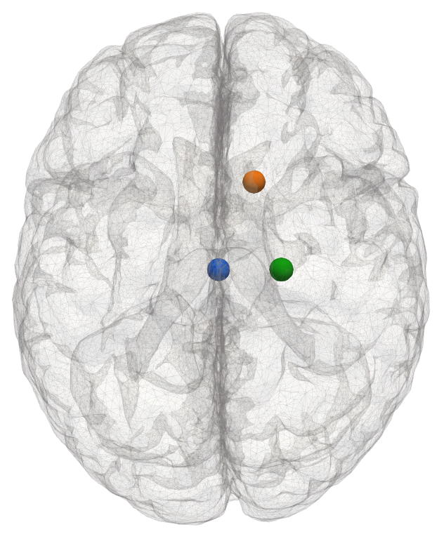
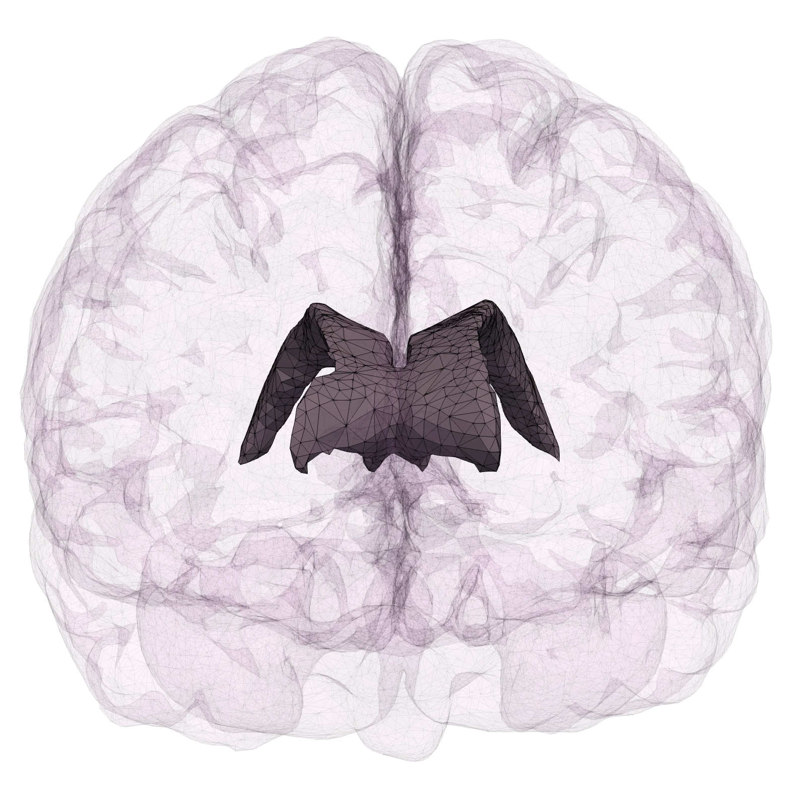
Figure 1: Left: The human brain computational mesh used in Section 6 with $99\,605$ cells and $29\,037$ vertices. View from top i.e. along the negative z-axis. The points $x_{0}$ (blue), $x_{1}$ (orange), $x_{2}$ (green) are marked with spheres. Right: The inner (ventricular) boundaries of the computational mesh. View from front i.e. along negative y-axis.

Symbol	Value(s)	Units	Reference
$\nu$	$0.4999$		Comparable with [26]
$E$	$1500$	Pa	Comparable with [13]
$c_{1}$	$3.9\times 10^{-4}$	Pa-1	[16, Table 2]
$c_{2},c_{4}$	$2.9\times 10^{-4}$	Pa-1	[16, Table 2]
$c_{3}$	$1.5\times 10^{-5}$	Pa-1	[16, Table 2]
$\alpha_{1}$	0.49		[16, Table 2]
$\alpha_{2},\alpha_{4}$	0.25		[16, Table 2]
$\alpha_{3}$	0.01		[16, Table 2]
$K_{1}$	$1.57\cdot 10^{-5}$	mm2 Pa-1 s-1	[36, Table 1]
$K_{2},K_{3},K_{4},$	$3.75\cdot 10^{-2}$	mm2 Pa-1 s-1	[36, Table 1]
$\xi_{2\leftarrow 4},\xi_{4\leftarrow 3},\xi_{4\leftarrow 1},\xi_{1\leftarrow 3}$	$1.0\times 10^{-6}$	Pa-1 s-1	Comparable with [24]
$\xi_{1\leftarrow 2},\xi_{2\leftarrow 3}$	$0.0$	Pa-1 s-1	[36]

Table 6: Material parameters used for the multiple network poroelasticity equations (1.1) with $A=4$ networks for the numerical experiments in Section 6. We remark that a wide range of parameter values can be found in the literature and the ones used here represents one sample set of representative values.

We consider the following set of boundary conditions for the system for all $t\in(0,T)$. All boundary pressure values are given in mmHg below, noting that $1$ mmHg $\approx 133.32$ Pa. We assume that the displacement is fixed on the outer boundary and prescribe a total stress on the inner boundary:

$$u=0\quad\text{on skull},\quad(C\varepsilon(u)-\operatorname{\textstyle\sum}_{j=1}^{4}\alpha_{j}p_{j}I)\cdot n=s\,n\quad\text{on ventricles},$$

where $n$ is the outward boundary normal and $s$ is defined as

$$s=-\sum_{j=1}^{4}\alpha_{j}\tilde{p}_{j},$$

where $\tilde{p}_{j}$ for $j=1,\dots,4$ are given below. We assume that the fluid in network 1 is in direct communication with the surrounding cerebrospinal fluid, and that a cerebrospinal fluid pressure is prescribed. In particular, we assume that the cerebrospinal fluid pressure pulsates around a baseline pressure of $5$ (mmHg) with a peak transmantle pressure difference magnitude of $\delta=0.012$ (mmHg):

$$p_{1}=5+2\sin(2\pi t)\quad\text{on skull},\quad p_{1}=5+(2+\delta)\sin(2\pi t)\equiv\tilde{p}_{1}\quad\text{on ventricles}.$$

We assume that a pulsating arterial blood pressure is prescribed at the outer boundary, while on the inner boundaries, we assume no arterial flux:

$$p_{2}=70+10\sin(2\pi t)\equiv\tilde{p}_{2}\quad\text{on skull},\quad\operatorname{\nabla}p_{2}\cdot n=0\quad\text{on ventricles}.$$

For the venous compartment, we assume that a constant pressure is prescribed at both boundaries:

$$p_{3}=6\equiv\tilde{p}_{3}\quad\text{on skull and ventricles}.$$

Finally, for the capillary compartment, we assume no flux at both boundaries:

$$\operatorname{\nabla}p_{4}\cdot n=0\quad\text{on skull and ventricles}.$$

We consider the following initial conditions:

$$u=0,\quad p_{1}=5,\quad p_{2}=70,\quad p_{3}=6,\quad p_{4}=(p_{2}+p_{3})/2\equiv\tilde{p}_{4},$$

and material parameters as reported in Table 6.

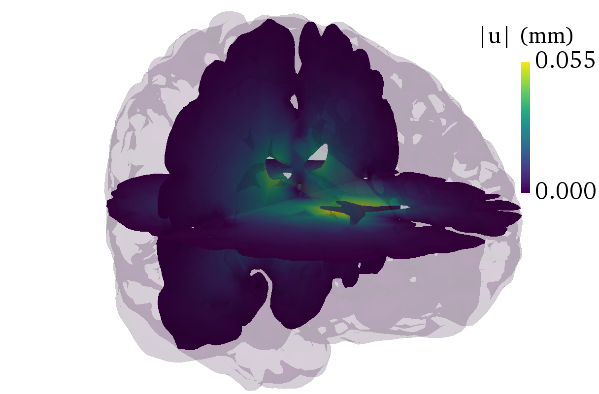
(a) Displacement magnitude $|u(\bar{t})|$

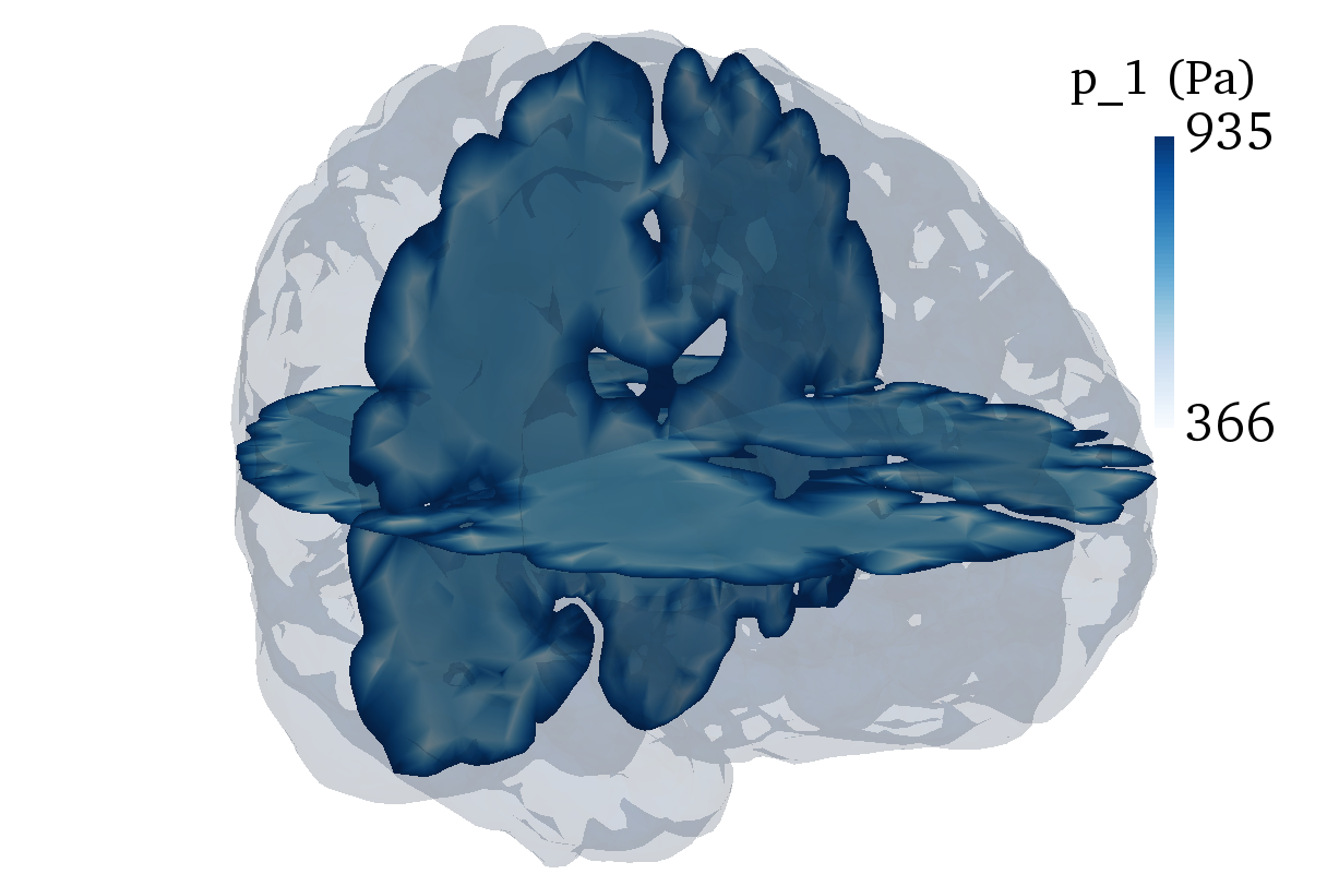
(b) Extracellular pressure $p_{1}(\bar{t})$

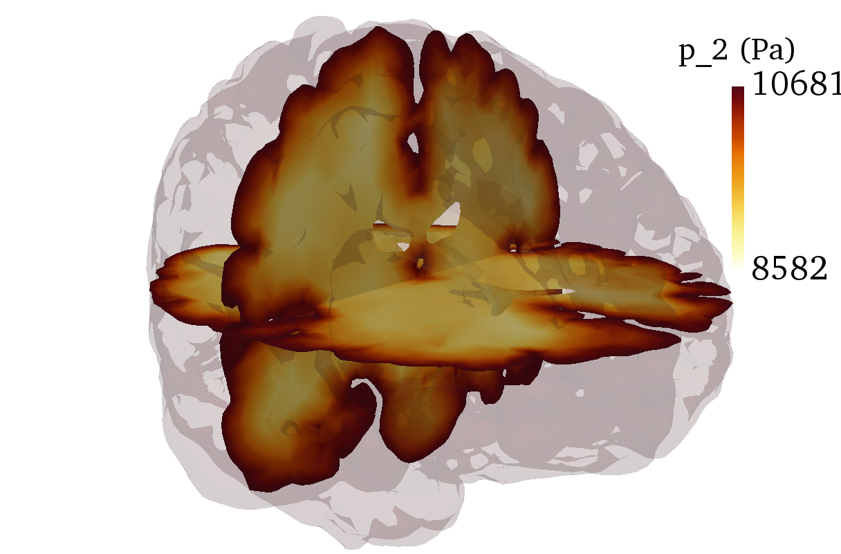
(c) Arterial pressure $p_{2}(\bar{t})$

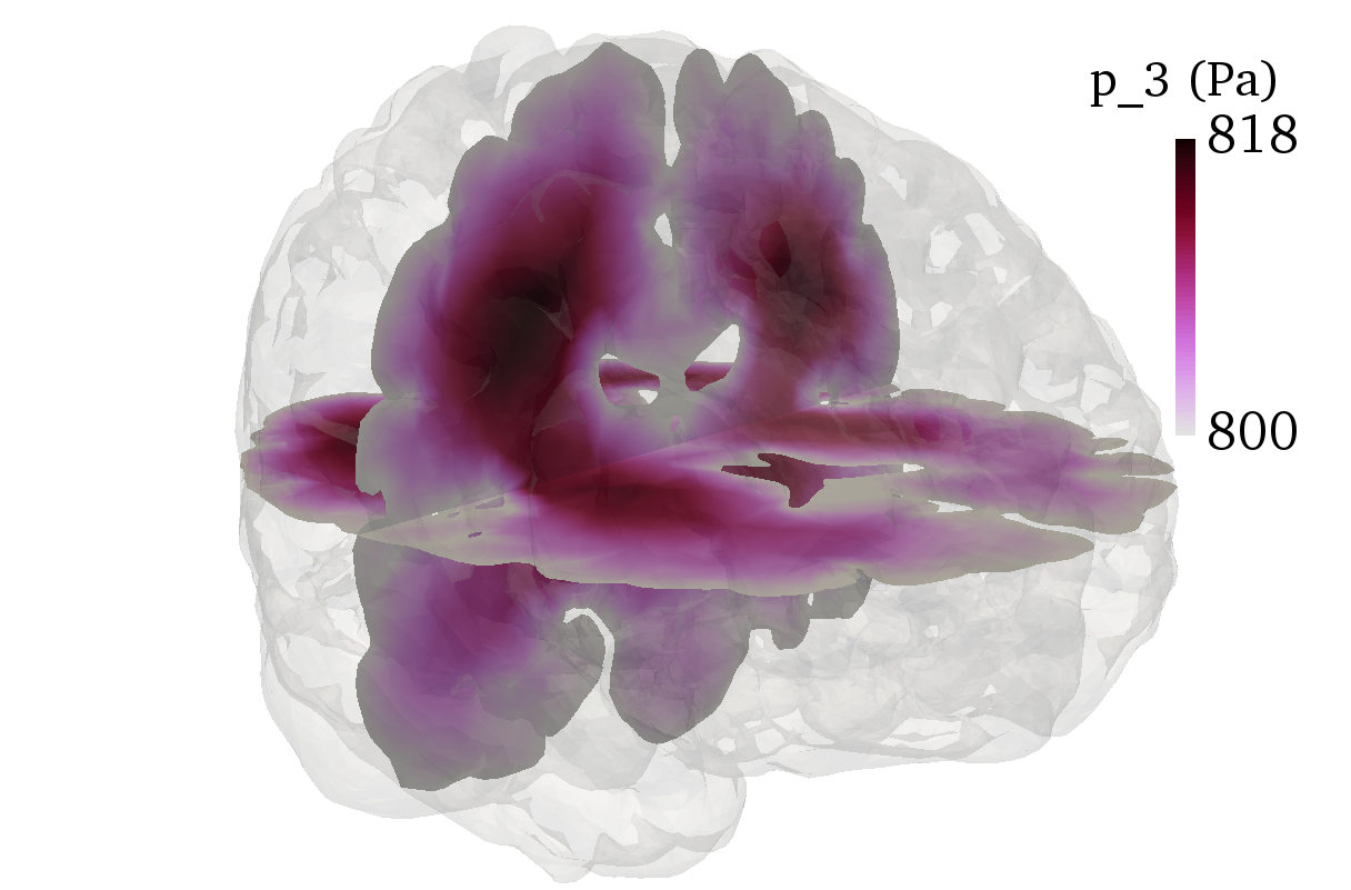
(d) Venous pressure $p_{3}(\bar{t})$

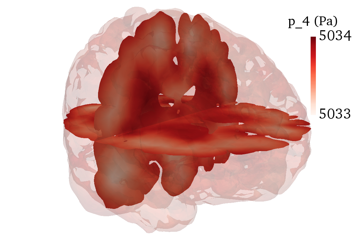
(e) Capillary pressure $p_{4}(\bar{t})$

Figure 2: Results of numerical experiment described in Section 6 using the total pressure formulation. Plots show slices of computed quantities at $\bar{t}=2.25$ (s) corresponding to the peak arterial inflow in the 2nd cycle. From left to right and top to bottom: (a) displacement magnitude $|u|$, (b) extracellular pressure $p_{1}$, (c) arterial blood pressure $p_{2}$, (d) venous blood pressure $p_{3}$ and (e) capillary blood pressure $p_{4}$.

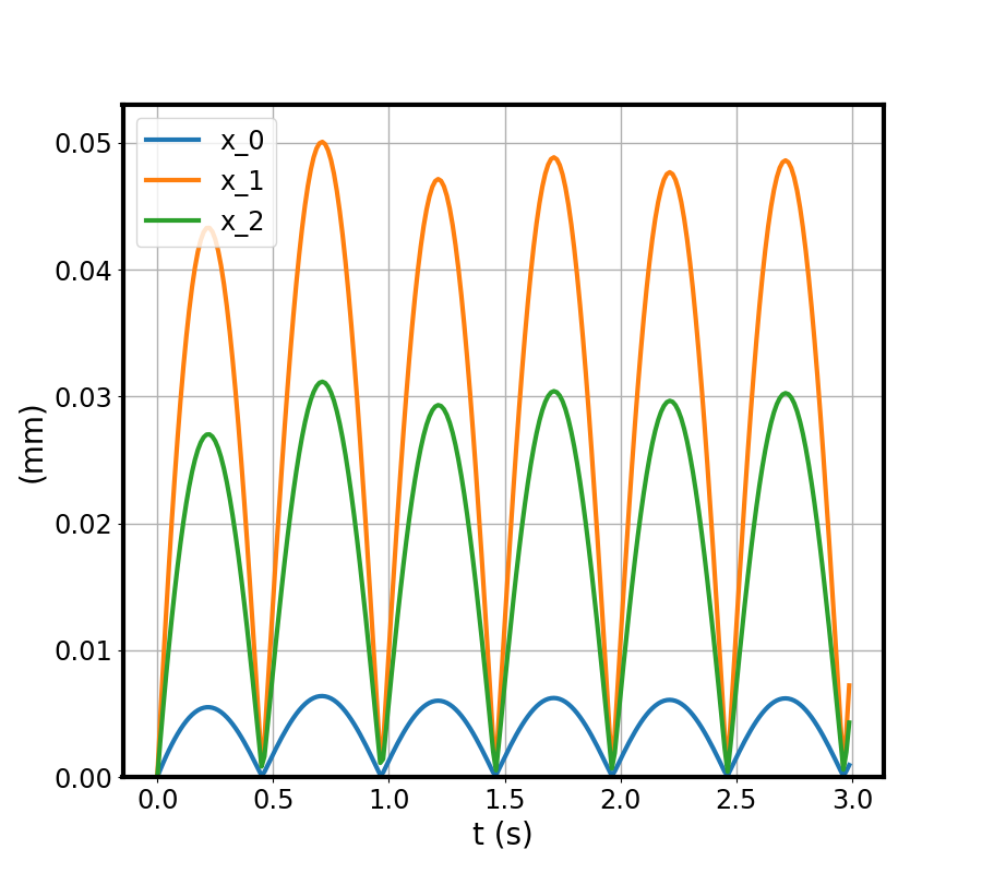
(a) Displacement magnitude $|u(x_{i})|$

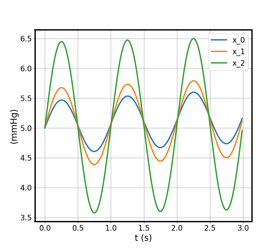
(b) Extracellular pressure $p_{1}(x_{i})$

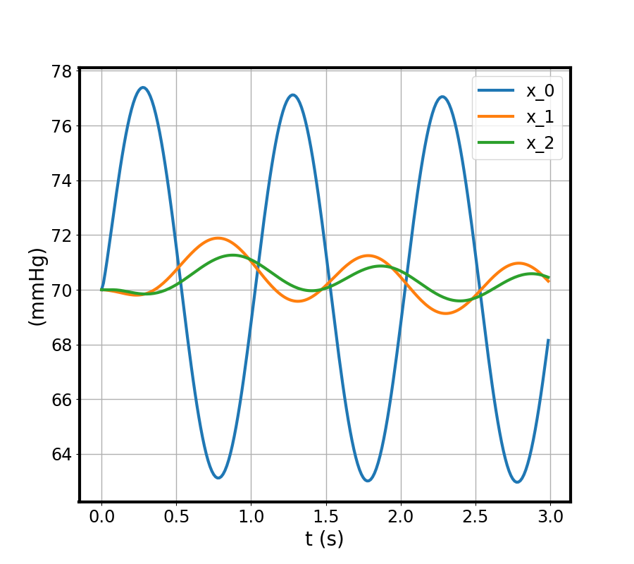
(c) Arterial pressure $p_{2}(x_{i})$

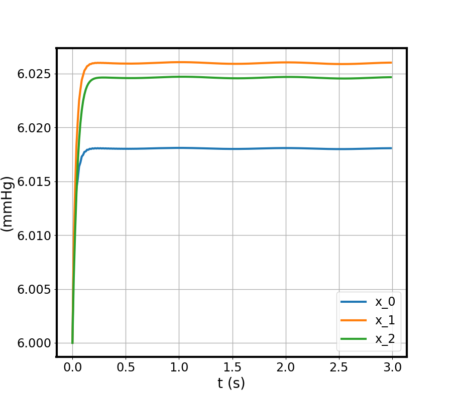
(d) Venous pressure $p_{3}(x_{i})$

(e) Capillary pressure $p_{4}(x_{i})$

Figure 3: Results of numerical experiment described in Section 6 using the total pressure formulation. Plots show computed quantities over time $t\in(0.0,3.0)$ for a set of three points $x_{0}$, $x_{1}$, $x_{2}$. See Figure 1 for the location and precise coordinates of the points $x_{i}$. From left to right and top to bottom: (a) displacement magnitude $|u|$, (b) extracellular pressure $p_{1}$, (c) arterial blood pressure $p_{2}$, (d) venous blood pressure $p_{3}$ and (e) capillary blood pressure $p_{4}$.

We computed the resulting solutions using the total pressure mixed finite element formulation with the lowest order Taylor-Hood type elements ($l=1$ and $l_{j}=1$ for $j=1,\dots,4$ in (4.4)), a Crank-Nicolson type discretization in time with time step $\Delta t=0.0125$ (s) over the time interval $(0.0,3.0)$ (s). The linear systems of equations were solved using a direct solver (MUMPS). For comparison, we also computed solutions with a standard mixed finite element formulation (as described and used in Example 1) and otherwise the same numerical set-up.

The numerical results using the total pressure formulation are presented in Figures 2 and 3. In particular, snapshots of the displacement and network pressures at peak arterial inflow in the 3rd cycle ($t=2.25$ (s)) are presented in Figure 2. Plots of the displacement magnitude and network pressures in a set of points versus time are presented in Figure 3.

We also compared the solutions computed using the total pressure and standard mixed finite element formulation. Plots of the displacement magnitude in a set of points over time are presented in Figure 4. We clearly observe that the computed displacements using the two formulations differ. For instance, the displacement magnitude in the point $x_{0}$ computed using the standard formulation is less than half the magnitude computed using the total pressure formulation. We also visually compared the pressures computed using the two formulations and found only minimal differences for this test case (data not shown for the standard formulation).

(a) Total pressure formulation

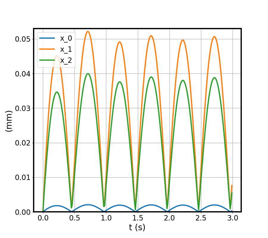
(b) ’Standard’ formulation

Figure 4: Comparison of displacements computed using the standard and total pressure formulation (cf. Section 6). Plots of displacement magnitude $|u(x_{i},t)|$ versus time $t$, for a set of points $x_{0},x_{1},x_{2}$ (see Figure 1 for the location and precise coordinates of the points $x_{i}$): (a) Total-pressure mixed finite element formulation, (b) Standard mixed finite element formulation (cf. Example 1). The computed displacements clearly differ between the two solution methods.

7 Conclusions

In this paper, we have presented a new mixed finite element formulation for the quasi-static multiple-network poroelasticity equations. Our formulation introduces a single additional scalar field unknown, the total pressure. We prove, via energy and semi-discrete a priori error estimates, that this formulation is robust in the limits of incompressibility ($\lambda\rightarrow\infty$) and vanishing storage coefficients ($c_{j}\rightarrow 0$), in contrast to standard formulations. Finally, numerical experiments support the theoretical results. For the numerical experiments presented here, we have used direct linear solvers. In future work, we will address iterative solvers and preconditioning of the MPET equations.

References

• [1] N. J. Abbott, M. E. Pizzo, J. E. Preston, D. Janigro, and R. G. Thorne, The role of brain barriers in fluid movement in the CNS: is there a ”glymphatic” system?, Acta Neuropathol., (2018), pp. 1–21.
• [2] G. Aguilar, F. Gaspar, F. Lisbona, and C. Rodrigo, Numerical stabilization of Biot’s consolidation model by a perturbation on the flow equation, Inter. J. Numer. Meth. Eng., 75 (2008), pp. 1282–1300.
• [3] M. Alnæs, J. Blechta, J. Hake, A. Johansson, B. Kehlet, A. Logg, C. Richardson, J. Ring, M. E. Rognes, and G. N. Wells, The FEniCS project version 1.5, Archive of Numerical Software, 3 (2015), pp. 9–23.
• [4] M. Bause, F. Radu, and U. Köcher, Space–time finite element approximation of the Biot poroelasticity system with iterative coupling, Comput. Methods in Appl. Mech. Eng., 320 (2017), pp. 745–768.
• [5] M. Bercovier and O. Pironneau, Error estimates for finite element method solution of the Stokes problem in the primitive variables, Numer. Math., 33 (1979), pp. 211–224, https://doi.org/10.1007/BF01399555.
• [6] L. Berger, R. Bordas, D. Kay, and S. Tavener, Stabilized lowest-order finite element approximation for linear three-field poroelasticity, SIAM J. Sci. Comp., 37 (2015), pp. A2222–A2245.
• [7] D. Boffi, Stability of higher order triangular Hood-Taylor methods for the stationary Stokes equations, Math. Models Methods Appl. Sci., 4 (1994), pp. 223–235, https://doi.org/10.1142/S0218202594000133.
• [8] D. Boffi, Three-dimensional finite element methods for the Stokes problem, SIAM J. Numer. Anal., 34 (1997), pp. 664–670, https://doi.org/10.1137/S0036142994270193.
• [9] D. Braess, Finite elements: Theory, fast solvers, and applications in solid mechanics (2nd edition), Cambridge University Press, 2001.
• [10] S. C. Brenner and L. R. Scott, The Mathematical Theory of Finite Element Methods, Springer, Third ed., 2008, https://doi.org/10.1016/0022-1236(78)90073-3.
• [11] F. Brezzi, On the existence, uniqueness and approximation of saddle-point problems arising from Lagrangian multipliers, Rev. Française Automat. Informat. Recherche Opérationnelle Sér. Rouge, 8 (1974), pp. 129–151.
• [12] F. Brezzi and R. S. Falk, Stability of higher-order Hood–Taylor methods, SIAM J. Numer. Anal., 28 (1991), pp. 581–590.
• [13] S. Budday, R. Nay, R. de Rooij, P. Steinmann, T. Wyrobek, T. C. Ovaert, and E. Kuhl, Mechanical properties of gray and white matter brain tissue by indentation, J. Mech. Behav. Biomed. Mater., 46 (2015), pp. 318–330.
• [14] L. C. Evans, Partial differential equations, vol. 19 of Graduate Studies in Mathematics, American Mathematical Society, Providence, RI, 1998.
• [15] Q. Fang, Mesh-based Monte Carlo method using fast ray-tracing in Plücker coordinates, Biomed. Opt. Express, 1 (2010), pp. 165–175.
• [16] L. Guo, J. C. Vardakis, T. Lassila, M. Mitolo, N. Ravikumar, D. Chou, M. Lange, A. Sarrami-Foroushani, B. J. Tully, Z. A. Taylor, et al., Subject-specific multi-poroelastic model for exploring the risk factors associated with the early stages of Alzheimer’s disease, Interface Focus, 8 (2018), p. 20170019.
• [17] X. Hu, C. Rodrigo, F. J. Gaspar, and L. T. Zikatanov, A nonconforming finite element method for the Biot’s consolidation model in poroelasticity, J. Comput. Appl. Math., 310 (2017), pp. 143–154, https://doi.org/10.1016/j.cam.2016.06.003.
• [18] J. J. Iliff, M. Wang, Y. Liao, B. A. Plogg, W. Peng, G. A. Gundersen, H. Benveniste, G. E. Vates, R. Deane, S. A. Goldman, et al., A paravascular pathway facilitates CSF flow through the brain parenchyma and the clearance of interstitial solutes, including amyloid-$\beta$, Sci. Transl. Med., 4 (2012), p. 147ra111.
• [19] N. A. Jessen, A. S. F. Munk, I. Lundgaard, and M. Nedergaard, The glymphatic system: a beginner’s guide, Neurochem. Res., 40 (2015), pp. 2583–2599.
• [20] J. Korsawe and G. Starke, A least-squares mixed finite element method for Biot’s consolidation problem in porous media, SIAM J. Numer. Anal., 43 (2005), pp. 318–339.
• [21] J. J. Lee, Robust error analysis of coupled mixed methods for Biot’s consolidation model, J. Sci. Comput., 69 (2016), pp. 610–632, https://doi.org/10.1007/s10915-016-0210-0.
• [22] J. J. Lee, Robust three-field finite element methods for Biot’s consolidation model in poroelasticity, BIT, (2017), https://doi.org/10.1007/s10543-017-0688-3.
• [23] J. J. Lee, K.-A. Mardal, and R. Winther, Parameter-robust discretization and preconditioning of Biot’s consolidation model, SIAM J. Sci. Comp., 39 (2017), pp. A1–A24, https://doi.org/10.1137/15M1029473.
• [24] C. Michler, A. Cookson, R. Chabiniok, E. Hyde, J. Lee, M. Sinclair, T. Sochi, A. Goyal, G. Vigueras, D. Nordsletten, et al., A computationally efficient framework for the simulation of cardiac perfusion using a multi-compartment Darcy porous-media flow model, Int. J. Numer. Method Biomed. Eng., 29 (2013), pp. 217–232.
• [25] M. A. Murad, V. Thomée, and A. F. Loula, Asymptotic behavior of semidiscrete finite-element approximations of Biot’s consolidation problem, SIAM J. Numer. Anal., 33 (1996), pp. 1065–1083.
• [26] T. Nagashima, N. Tamaki, S. Matsumoto, B. Horwitz, and Y. Seguchi, Biomechanics of hydrocephalus: a new theoretical model, Neurosurgery, 21 (1987), pp. 898–904.
• [27] J. M. Nordbotten, T. Rahman, S. I. Repin, and J. Valdman, A posteriori error estimates for approximate solutions of the Barenblatt-Biot poroelastic model, Comput. Methods Appl. Math., 10 (2010), pp. 302–314.
• [28] R. Oyarzúa and R. Ruiz-Baier, Locking-free finite element methods for poroelasticity, SIAM J. Numer. Anal., 54 (2016), pp. 2951–2973.
• [29] P. J. Phillips and M. F. Wheeler, A coupling of mixed and continuous Galerkin finite element methods for poroelasticity. I. The continuous in time case, Comput. Geosci., 11 (2007), pp. 131–144, https://doi.org/10.1007/s10596-007-9045-y.
• [30] E. Piersanti and M. E. Rognes, Supplementary material (code) for A mixed finite element method for nearly incompressible multiple- network poroelasticity’ by J. J. Lee, E. Piersanti, K.-A. Mardal and M. E. Rognes., Apr. 2018, https://doi.org/10.5281/zenodo.1215636.
• [31] C. Rodrigo, X. Hu, P. Ohm, J. Adler, F. J. Gaspar, and L. Zikatanov, New stabilized discretizations for poroelasticity and the Stokes’ equations, arXiv preprint arXiv:1706.05169, (2017).
• [32] R. E. Showalter, Diffusion in poro-elastic media, J. Math. Anal. Appl., 251 (2000), pp. 310–340, https://doi.org/10.1006/jmaa.2000.7048, https://doi.org/10.1006/jmaa.2000.7048.
• [33] R. E. Showalter and B. Momken, Single-phase flow in composite poroelastic media, Math. Methods Appl. Sci., 25 (2002), pp. 115–139, https://doi.org/10.1002/mma.276.
• [34] C. Taylor and P. Hood, A numerical solution of the Navier-Stokes equations using the finite element technique, Comput. Fluids, 1 (1973), pp. 73–100.
• [35] B. J. Tully and Y. Ventikos, Cerebral water transport using multiple-network poroelastic theory: application to normal pressure hydrocephalus, J. Fluid Mech., 667 (2011), pp. 188–215.
• [36] J. C. Vardakis, D. Chou, B. J. Tully, C. C. Hung, T. H. Lee, P.-H. Tsui, and Y. Ventikos, Investigating cerebral oedema using poroelasticity, Med. Eng. Phys., 38 (2016), pp. 48–57.
• [37] S.-Y. Yi, Convergence analysis of a new mixed finite element method for Biot’s consolidation model, Numer. Methods Partial Differential Equations, 30 (2014), pp. 1189–1210, https://doi.org/10.1002/num.21865.
• [38] S.-Y. Yi, A study of two modes of locking in poroelasticity, SIAM J. Numer. Anal., 55 (2017), pp. 1915–1936.
• [39] K. Yosida, Functional Analysis, Springer Classics in Mathematics, Springer-Verlag, 6th ed., 1980.