Perturbations of spiky strings in $AdS_{3}$

Abstract:

Perturbations of a class of semiclassical spiky strings in three dimensional Anti-de Sitter (AdS) spacetime, are investigated using the well-known Jacobi equations for small, normal deformations of an embedded timelike surface. We show that the equation for the perturbation scalar which governs the behaviour of such small deformations, is a special case of the well-known Darboux-Treibich-Verdier (DTV) equation. The eigenvalues and eigensolutions of the DTV equation for our case are obtained by solving certain continued fractions numerically. These solutions are thereafter utilised to further demonstrate that there do exist finite perturbations of the AdS spiky strings. Our results therefore establish that the spiky string configurations in $AdS_{3}$ are indeed stable against small fluctuations. Comments on future possibilities of work are included in conclusion.

1 Introduction

In the early days of string theory, rigidly rotating strings arose in the work of Burden and Tassie [1, 2, 3] primarily as stringy models for exotic mesons and glue balls. Gravitational radiation from this particular class of strings (viewed as cosmic strings) was discussed in [4]. Later, Embacher [5] obtained the complete class of such solutions in flat spacetime, with rigid rotation about a fixed axis. Further work can be found in [6, 7, 8, 9, 10].

In its modern avatar, such rigidly rotating strings have been renamed as spiky strings. Their importance and relevance today is largely in the context of the AdS/CFT correspondence [11]. More than a decade ago, the spiky string solutions appeared, through the seminal work by Kruczenski [12], as a potential gravity dual to higher twist operators in string theory. In string theory and in AdS/CFT, the solutions of interest are closed strings with spikes (in cosmic string nomenclature these are called ‘cusps’). The semiclassical aspect of these solutions arise through evaluating their energies, angular momenta and finding relations between them [13].

In providing meaningful input towards the realization of the gauge-gravity duality, the emergence of integrability on both sides have been quite useful and important. Classical and quantum integrability of the ${\cal N}$ = 4 Supersymmetric Yang-Mills (SYM) theory in the planar limit is mainly useful for the remarkable advances in understanding the theory [14, 15, 16]. The nonlocal conserved charges found on the string side [17, 18] appear to have a counterpart in planar gauge theory at weak coupling within the spin-chain formulation for the dilatation operator. The integrability of the ${\cal N}$ = 4 SYM theory should not only have important consequences for the spectrum of anomalous dimensions of gauge-invariant single trace operators but also for other observables, e.g. the Wilson loops. One such class of string states in the string theory side are the so called spiky strings, which have been shown to be dual to higher twist operators in ${\cal N}$ = 4 SYM theory with each spike corresponding to a particle on the field theory side of the correspondence. Large angular momentum is provided by a large number of covariant derivatives acting on the fields which produce the above-mentioned particles. The total number of derivatives is distributed equally amongst the fields for these solutions. A large class of such spiky strings in various asymptotically AdS and non-AdS backgrounds have been studied, for example, in [12],[19],[20],[21],[22],[23],[24].

Given the above-stated importance of the spiky strings, it is worthwhile to look at the geometric properties of such string configurations from the world sheet view point. To this end, following our earlier work [25] we study normal deformations (linearized) about the classical solutions in $AdS_{3}$. Earlier work in [26] dealt with computation of quantum corrections to the energy spectrum, by expanding the supersymmetric action to quadratic order in fluctuations about the classical solution. The linearized perturbations of semiclassical strings are extremely instructive in matching the duality beyond the leading order classical solutions. The main motivations behind the perturbative solutions are multi-fold. On one hand, it helps in studying the stability properties of the string dynamics of the closed strings, and finding the quantum string corrections to the Wilson loop expectation value for the open string solutions and on the other hand, it helps us in determining the physical properties of topological defects.

Motivated by various studies on general classes of rotating strings in $AdS_{5}\times S^{5}$, in this paper, we investigate the classical stability of the spiky strings in $AdS_{3}$ using the well-known Jacobi equations [27],[28],[29], [30] which govern normal deformations of an embedded surface. Apart from [25], related recent work on such perturbations can be found in [31]. The rest of this article is organised as follows. In Section 2, we briefly summarize the two different embeddings of the worldsheet and the spiky string solution in $AdS_{3}$. Section 3 is devoted to a study of the perturbation equation which turns out to be a special case of the Darboux-Treibich-Verdier equation in mathematical physics. We also discuss, in Section 3, the numerical evaluation of the eigenvalues and eigenfunctions, obtained by solving an infinite continued fraction numerically. Plots of the perturbations $\delta x^{i}$ are shown for various eigenvalues and the issue of stability is addressed. Our final concluding remarks appear in Section 4.

2 Spiky strings in $AdS_{3}$: Kruczenski and Jevicki-Jin embeddings

The bosonic string worldsheet embedded in a $N$ dimensional curved spacetime with background metric functions $g_{ij}(x)$, is described by the well-known Nambu-Goto action given as,

$$S=-T\int d\tau\,\,d\sigma\sqrt{-\gamma}=-T\int d\tau\,\,d\sigma\sqrt{(\dot{x}\cdot x^{\prime})^{2}-\dot{x}^{2}{x^{\prime}}^{2}}\ .$$ (1)

Here $\gamma$ denotes the determinant of the induced metric $\gamma_{ab}=g_{ij}\partial_{a}x^{i}\partial_{b}x^{j}$ ($a,b=\sigma,\tau$). The $x^{i}(\tau,\sigma)$ are functions which describe the profile of the string worldsheet, as embedded in the target spacetime. $T$ denotes the string tension. We have used the notation: $\dot{x}=\partial_{\tau}x$,  $x^{\prime}=\partial_{\sigma}x$,   $(\dot{x}\cdot x^{\prime})=g_{ij}{\dot{x}}^{i}\,{x^{\prime}}^{j}$,  ${\dot{x}}^{2}=g_{ij}{\dot{x}}^{i}\,{\dot{x}}^{j}$ and ${x^{\prime}}^{2}=g_{ij}{x^{\prime}}^{i}\,{x^{\prime}}^{j}$. Let us now turn to spiky strings in AdS spacetime in three dimensions. The AdS line element is given as

$$ds^{2}=-\cosh^{2}\rho\,\,dt^{2}+d\rho^{2}+\sinh^{2}\rho\,\,d\theta^{2}\ .$$ (2)

We use the following embedding

$$t=\tau,\ \ \theta=\omega\tau+\sigma,\ \ \rho=\rho(\sigma)\ .$$ (3)

Using the equations of motion from the action (1) one can get an equation of $\rho(\sigma)$ given as,

$$\rho^{\prime}=\frac{1}{2}\frac{\sinh 2\rho}{\sinh 2\rho_{0}}\frac{\sqrt{\sinh^{2}2\rho-\sinh^{2}2\rho_{0}}}{\sqrt{\cosh^{2}\rho-\omega^{2}\sinh^{2}\rho}}\,\,,$$ (4)

where $\rho_{0}$ is the integration constant. From the expression of $\rho^{\prime}$ it is clear that $\rho$ varies from a minimum value $\rho_{0}$ to a maximum value $\rho_{1}=\mbox{arccoth}\,\omega$. At $\rho=\rho_{1}$, $\rho^{\prime}$ diverges indicating the presence of a spike and at $\rho=\rho_{0}$, $\rho^{\prime}$ vanishes, indicating the bottom of the valley between spikes. To get a solution with $n$ spikes one has to glue $2n$ of the arc segments and the angle between cusp and valley is $\frac{2\pi}{2n}$. Figures 1 and 2 show such spiky string configurations as embedded in an Euclidean space, with ten and three spikes respectively [12].

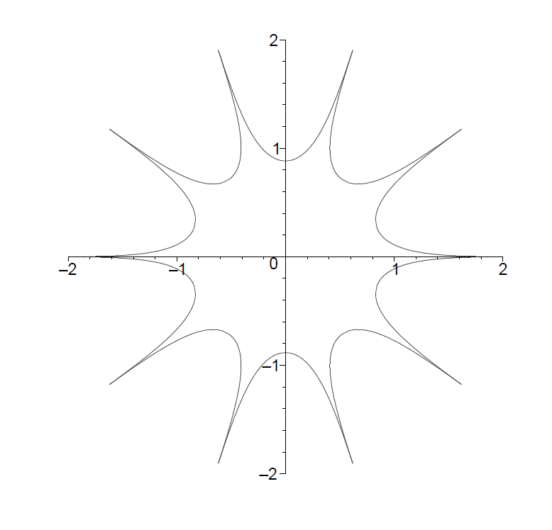
Figure 1: The Kruczenski spiky string in ($\rho,\theta$) plane for $n=10$ spikes with $\rho_{1}=2.0~{}\&~{}\rho_{0}=0.88266$ .

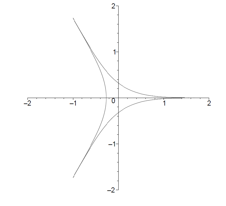
Figure 2: The Kruczenski spiky string in ($\rho,\theta$) plane for $n=3$ spikes with $\rho_{1}=2.0~{}\&~{}\rho_{0}=0.2688$ .

In conformal gauge, we have

$$g_{ij}({\dot{x}}^{i}{\dot{x}}^{j}+{x^{\prime}}^{i}{x^{\prime}}^{j})=0,\hskip 21.68121ptg_{ij}{\dot{x}}^{i}{x^{\prime}}^{j}=0\ .$$ (5)

In such a gauge, the string equations of motion obtained by varying the action with respect to $x^{i}$, take the form:

$${\ddot{x}}^{i}-{x^{i^{\prime\prime}}}+\Gamma^{i}_{jk}\left({\dot{x}}^{j}{\dot{x}}^{k}-{x}^{j\prime}{x}^{k\prime}\right)=0\ .$$ (6)

We may also choose the following embedding due to Jevicki and Jin [32]:

$$t=\tau+f(\sigma),\hskip 7.22743pt\rho=\rho(\sigma),\hskip 7.22743pt\theta=\omega\tau+g(\sigma)\ .$$ (7)

As we shall see, this embedding will be useful in our calculations later.

With the Jevicki-Jin ansatz mentioned above, we find that the tangent vector to the worldsheet is given as:

$$e^{i}_{\tau}=\left(1,0,\omega\right)\hskip 14.45377pt;\hskip 14.45377pte^{i}_{\sigma}=\left(f^{\prime},\rho^{\prime},g^{\prime}\right)\ .$$ (8)

The equations of motion and the Virasoro constraints turn out to be

$$f^{\prime}(\sigma)=\frac{\omega\sinh 2\rho_{0}}{2\cosh^{2}\rho}\hskip 14.45377pt;\hskip 14.45377ptg^{\prime}(\sigma)=\frac{\sinh 2\rho_{0}}{2\sinh^{2}\rho}$$ (9)

$${\rho^{\prime}}^{2}(\sigma)=\frac{\left(\cosh^{2}\rho-\omega^{2}\sinh^{2}\rho\right)\left(\sinh^{2}2\rho-\sinh^{2}2\rho_{0}\right)}{\sinh^{2}2\rho}\ .$$ (10)

The solution of the $\rho$ equation is given in terms of Jacobian elliptic functions

$$\rho(\sigma)=\frac{1}{2}\cosh^{-1}\left(\cosh 2\rho_{1}\,\,{\rm cn}^{2}(u,k)+\cosh 2\rho_{0}\,\,{\rm sn}^{2}(u,k)\right)\,\,,$$ (11)

here ${\rm sn}(u,k)$ and ${\rm cn}(u,k)$ are the Jacobi elliptic functions with modular parameter $k^{2}$ and $u$ & $k$ are defined as

$$u=\sqrt{\frac{\cosh 2\rho_{1}+\cosh 2\rho_{0}}{\cosh 2\rho_{1}-1}}\,\,\sigma=\zeta\sigma\,\,,$$ (12)

$$k=\sqrt{\frac{\cosh 2\rho_{1}-\cosh 2\rho_{0}}{\cosh 2\rho_{1}+\cosh 2\rho_{0}}}\ .$$ (13)

It is possible to write down $f$ and $g$ as well but we do not need them here. Explicit expressions are available in [32]. We now turn towards examining the stability of the string configurations by studying their normal deformations.

3 Perturbations and stability of spiky strings in $AdS_{3}$

Before investigating the perturbation equations for our specific solutions, let us briefly recall the well-known Jacobi equations which deal with perturbations of extremal worldsheets.

3.1 Jacobi equations for extremal surfaces

Given that $x^{i}(\tau,\sigma)$ are the embedding functions and $g_{ij}$ the background metric, the tangent vectors to the worldsheet are

$$e^{i}_{\tau}=\partial_{\tau}x^{i},\hskip 14.45377pte^{i}_{\sigma}=\partial_{\sigma}x^{i}.$$ (14)

Thus, the induced line element turns out to be,

$$\gamma_{ab}=g_{ij}e^{i}_{a}e^{j}_{b}\ ,$$ (15)

where the $a,b...$ denote worldsheet indices (here $\tau$, $\sigma$). The worldsheet normals $n^{i}_{(\alpha)}$ satisfy the relations

$$g_{ij}n^{i}_{(\alpha)}n^{j}_{(\beta)}=\delta_{\alpha\beta},\hskip 14.45377ptg_{ij}n^{i}_{(\alpha)}e^{j}_{a}=0\ ,$$ (16)

where $\alpha=1..,N-2$ and $N$ is the dimension of the background spacetime. The last condition holds for all $\alpha$ and $a$. Extrinsic curvature tensor components $K_{ab}^{(\alpha)}$ along each normal $n^{i}_{(\alpha)}$ of the embedded worldsheet are

$$K_{ab}^{(\alpha)}=-g_{ij}(e^{k}_{a}\nabla_{k}e^{i}_{b})n^{j(\alpha)}\ .$$ (17)

The equations of motion lead to the condition, $K^{(\alpha)}=\gamma^{ab}K_{ab}^{(\alpha)}=0$ for an extremal worldsheet. Thus extremal surfaces are those for which the trace of the extrinsic curvature tensor along each normal is zero. Normal deformations are denoted as $\phi^{(\alpha)}$ along each normal. Therefore, the deformations constitute a set of scalar fields. More explicitly, the deformation of each coordinate is

$$\delta x^{i}=\phi^{(\alpha)}n^{i}_{(\alpha)}\ ,$$ (18)

which is the perturbation of the worldsheet (i.e. $x^{i}\rightarrow x^{i}+\delta x^{i}$). For a worldsheet with $\gamma^{ab}K_{ab}^{(\alpha)}=0$ satisfying the equations of motion and the Virasoro constraints, the scalars $\phi^{i}_{(\alpha)}$ satisfy the Jacobi equations given as

$$\frac{1}{\Omega^{2}}\left(-\frac{\partial^{2}}{\partial\tau^{2}}+\frac{\partial^{2}}{\partial\sigma^{2}}\right)\phi^{(\alpha)}+\left(M^{2}\right)^{(\alpha)}_{(\beta)}\phi^{(\beta)}=0\ ,$$ (19)

where

$$\left(M^{2}\right)^{(\alpha)}_{(\beta)}=K_{ab}^{(\alpha)}K^{ab}_{(\beta)}+R_{ijkl}e^{j}_{a}e^{l\,\,a}n^{i\,\,(\alpha)}n^{k}_{(\beta)}\ ,$$ (20)

and $\Omega^{2}(\tau,\sigma)$ is the conformal factor of the conformally flat form of the worldsheet line element. The Jacobi equations are obtianed by constructing the second variation of the worldsheet action. Thus, solving these equations for the perturbation scalars one can analyse the stability properties of the extremal worldsheet. In other worlds, a stable worldsheet will correspond to an oscillatory character for the $\delta x^{i}$ defined above.

Note further that the Jacobi equations are like a family of coupled, variable ‘mass’ wave equations for the scalars $\phi^{(\alpha)}$. They are a generalisation of the familiar geodesic deviation equation for geodesic curves in a Riemannian geometry. Usually, these equations are quite complicated and not easily solvable, even for the simplest cases. It turns out that for the string configurations under consideration here, we do find analytical solutions.

In a more general context, the worldsheet covariant derivative does have a term arising from the extrinsic twist potential (normal fundamental form) which is given as: $\omega_{a}^{\,\,\alpha\beta}=g_{ij}\,\left(e^{k}_{a}\nabla_{k}\,n^{i\,\alpha}\right)\,n^{j\,\beta}$. For codimension one surfaces, i.e. hypersurfaces (as is the case here), the $\omega_{a}^{\alpha\beta}$ are all identically zero.

3.2 The case of spiky strings in $AdS_{3}$

Let us now turn to the string configurations mentioned earlier: i.e. the $AdS_{3}$ spiky strings. To proceed, we first write down the normal, induced metric and extrinsic curvature for the world sheet configurations in the Jevicki-Jin gauge stated earlier.

The normal to the worldsheet is given as:

$$n^{i}=\left(\frac{\omega\rho^{\prime}\tanh\rho}{\cosh^{2}\rho-\omega^{2}\sinh^{2}\rho},-\frac{\sinh 2\rho_{0}}{\sinh 2\rho},\frac{\rho^{\prime}\coth\rho}{\cosh^{2}\rho-\omega^{2}\sinh^{2}\rho}\right)\,\,.$$ (21)

Using the expression of $\rho(\sigma)$ one can write the normal in the following form:

$$n^{i}=(n^{0},~{}n^{1},~{}n^{2})\,,$$ (22)

where,

$$n^{0}=\frac{\omega~{}\sqrt{\delta~{}\gamma~{}{\rm sn}^{2}(u,k)-2\delta~{}(\delta+1)+\frac{\eta~{}\delta}{{\rm sn}^{2}(u,k)}}}{\alpha-\gamma~{}{\rm sn}^{2}(u,k)}\,\,,$$ (23)

$$n^{1}=\frac{-\sinh 2\rho_{0}}{\sqrt{\gamma^{2}~{}{\rm sn}^{4}(u,k)-2\gamma~{}(\delta+1)~{}{\rm sn}^{2}(u,k)+\alpha~{}\delta}}\,\,,$$ (24)

$$n^{2}=\frac{\sqrt{\delta~{}\gamma~{}{\rm sn}^{2}(u,k)-2\delta~{}(\delta+1)+\frac{\eta~{}\delta}{{\rm sn}^{2}(u,k)}}}{\delta-\gamma~{}{\rm sn}^{2}(u,k)}\,\,,$$ (25)

and $\alpha,~{}\delta,~{}\gamma~{}\&~{}\eta$ are defined as follows

$$\alpha=1+\cosh 2\rho_{1},~{}\delta=\cosh 2\rho_{1}-1,~{}\gamma=\cosh 2\rho_{1}-\cosh 2\rho_{0},~{}\&~{}\eta=\cosh 2\rho_{1}+\cosh 2\rho_{0}\ .$$

The extrinsic curvature tensor turns out to be

$$K_{ab}=\begin{pmatrix}\frac{1-\omega^{2}}{2}\sinh 2\rho_{0}&-\omega\cr-\omega&\frac{1-\omega^{2}}{2}\sinh 2\rho_{0}\end{pmatrix}.$$ (26)

The induced metric is given as:

$$ds^{2}=\left(\cosh^{2}\rho-\omega^{2}\sinh^{2}\rho\right)\left(-d\tau^{2}+d\sigma^{2}\right).$$ (27)

Hence the quantity $K_{ab}K^{ab}$ is given as:

$$K_{ab}K^{ab}=2\frac{\left(1-\omega^{2}\right)^{2}\sinh^{2}\rho_{0}\cosh^{2}\rho_{0}-\omega^{2}}{\left(\cosh^{2}\rho-\omega^{2}\sinh^{2}\rho\right)^{2}}=\frac{P}{\Omega^{4}}\,\,,$$ (28)

where $P=2\left(1-\omega^{2}\right)^{2}\sinh^{2}\rho_{0}\cosh^{2}\rho_{0}-\omega^{2}$ and $\Omega^{2}=\left(\cosh^{2}\rho-\omega^{2}\sinh^{2}\rho\right)$. Similarly one can write down the contribution from the Riemann tensor term in the perturbation equation as follows

$$R_{ijkl}e^{j}_{a}e^{l\,\,a}n^{i\,\,(\alpha)}n^{k}_{(\beta)}=-2~{}\delta^{\alpha}_{\beta}\ .$$ (29)

Using all of the above-stated quantities which appear in the perturbation equation and after some lengthy algebra, one arrives at the following equation for the perturbation scalar $\phi$

$$\left(-\frac{\partial^{2}}{\partial\tau^{2}}+\frac{\partial^{2}}{\partial\sigma^{2}}\right)\phi+\left[-2\Omega^{2}+\frac{P}{\Omega^{2}}\right]\phi=0\,\,.$$ (30)

Let us now use the functional form of $\rho(\sigma)$ and the ansatz

$$\phi(\tau,\sigma)=\epsilon e^{i\beta\tau}R(\sigma)\,\,,$$ (31)

where $\beta$ will be the eigenvalue and $\epsilon$, a constant which we may relate to the amplitude of the perturbation. It must be emphasized that $\epsilon$ has to be small in value (i.e. $\epsilon<<1$) in order to ensure that the deformation is genuinely a perturbation. With the above ansatz for $\phi(\tau,\sigma)$ one can reduce the perturbation equation to an equation for $R(\sigma)$ given as:

$$\frac{d^{2}R}{du^{2}}+\left[\beta_{1}^{2}-2\left(k^{2}{\rm sn}^{2}(u,k)+\frac{1}{{\rm sn}^{2}(u,k)}\right)\right]R=0\,\,,$$ (32)

or

$$\frac{d^{2}R}{du^{2}}+\left[\beta_{1}^{2}-V(u)\right]R=0\,\,,$$ (33)

where $\beta_{1}^{2}=\frac{\beta^{2}}{\zeta^{2}}$, $u=\zeta\sigma$ (see Eqn. (12) for $\zeta$) and

$$V(u)=2\left(k^{2}{\rm sn}^{2}(u,k)+\frac{1}{{\rm sn}^{2}(u,k)}\right).$$ (34)

Eqn. (32) is a special case of the well-known Darboux-Treibich-Verdier (DTV) equation [33], [35] of mathematical physics. In general, the DTV equation has the following form:

$$\frac{d^{2}R}{dx^{2}}+(h-V(x))R=0\,\,,$$ (35)

with $V(x)$ given as:

$$\begin{split}V(x)&=\nu~{}(\nu+1)k^{2}~{}{\rm sn}^{2}(x,k)~{}+~{}\mu~{}(\mu+1)k^{2}~{}\frac{{\rm cn}^{2}(x,k)}{{\rm dn}^{2}(x,k)}~{}+\eta~{}(\eta+1)\frac{{\rm dn}^{2}(x,k)}{{\rm cn}^{2}(x,k)}\\ &+\xi~{}(\xi+1)\frac{1}{{\rm sn}^{2}(x,k)}\ .\end{split}$$ (36)

The potential $V(x)$ in the DTV equation is a periodic potential which includes the well-studied Lamé potential as a special case. Our equation is another special case of Eqn. (36) with $\nu=\xi=1$ and $\mu=\eta=0$ with period $2K$ where $K$ is defined as follows:

$$K=\int_{0}^{\frac{\pi}{2}}\frac{d\psi}{1-k^{2}\sin^{2}{\psi}}\,\ .$$ (37)

In Figures 3 and 4, we show the nature of our potential for the cases with ten and three spikes, respectively. Notice these are well–like potentials with a flat bottom (much like a generalisation of a harmonic oscillator potential with added anharmonicities). It is therefore obvious that there will be bound state solutions which will correspond to the normal mode fluctuations of the spiky string.

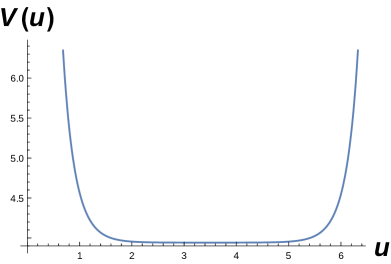
Figure 3: Plot of the potential $V(u)$ for one period range.

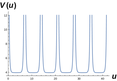
Figure 4: Plot of the potential $V(u)$ for more than one period range.

We will now move on to constructing solutions of the DTV equation (for our special case) and thereafter analyse the perturbations. This will lead us towards figuring out whether the spiky string configurations in $AdS_{3}$ are indeed stable or not.

3.3 Solving the Jacobi equation and the stability issue

Various forms of the linearly independent general solutions to the DTV equation exist in the literature. The earliest reference dates back to 1883 in a couple of articles by the mathematician Comte de Sparre [33, 34], who seems to have studied the DTV equation and its special cases in great detail. More recently, in work by Matveev and Smirnov [35] (who have rediscovered the work of Sparre), the general solutions have been written down using products of Jacobi and other Theta ($\Theta$) functions. We will however look at a series solution obtained recently in the article by Chiang et al [36] which turns out to be quite useful in obtaining the eigenfunctions and eigenvalues for our special case. This, as we shall see, further helps in understanding the stability issue of spiky strings in $AdS_{3}$.

A series solution of the general DTV equation ( $\xi\neq-\frac{3}{2},-\frac{5}{2}$) as pointed out in [36] is given as:

$${\rm sn}^{\xi+1}(u,k){\rm cn}^{\eta+1}(u,k){\rm dn}^{\mu+1}(u,k)\sum_{m=0}^{\infty}C_{m}{\rm sn}^{2m}(u,k)\ .$$ (38)

This expansion is known as a local Darboux solution and denoted as $Dl(\xi,\eta,\mu,\nu;h;u,k)$ where the $C_{m}$ satisfies the following recursion relation:

$$\begin{split}&(2m+2)(2m+2\xi+3)C_{m+1}\\ &+\{h-[2m+\eta+\xi+2]^{2}-k^{2}[2m+\mu+\xi+2]^{2}+(k^{2}+1)(\xi+1)^{2}\}C_{m}\\ &+k^{2}(2m+\xi+\eta+\mu+\nu+2)(2m+\xi+\eta+\mu-\nu+1)C_{m-1}=0\ .\end{split}$$ (39)

For simplicity, one may define

$$M_{m}(\xi):=(2m+2)(2m+2\xi+3);$$

$$L_{m}(\xi,\,\eta,\mu;h;k):=h-[2m+\eta+\xi+2]^{2}-k^{2}[2m+\mu+\xi+2]^{2}+(k^{2}+1)(\xi+1)^{2};$$

$$K_{m}(\xi,\eta,\mu,\nu;k):=k^{2}(2m+\xi+\eta+\mu+\nu+2)(2m+\xi+\eta+\mu-\nu+1)$$

so that (39) takes the form

$$M_{m}C_{m+1}+L_{m}C_{m}+K_{m}C_{m-1}=0\ .$$ (40)

We state below the content of two theorems regarding the convergence of $Dl(\xi,\eta,\mu,\nu;h;u,k)$ [36].

The first of these theorems as quoted in [36] states the following. If there exists a positive integer $q$ such that either

$$\xi+\eta+\mu+\nu=-2q-4\quad\mbox{ or }\quad\xi+\eta+\mu-\nu=-2q-3,$$ (41)

holds, then there exist $q+1$ values $h_{0},\,\cdots,\,h_{q}$ of $h$ such that the series $Dl(\xi,\eta,\mu,\nu;h_{j};u,k)$ ($j=0,1,\cdots,q$) terminates and yields a polynomial.

In the second theorem, the following result is stated. Suppose that $Dl(\xi,\eta,\mu,\nu;h;u,k)$ is non-terminating, i.e., not a Darboux polynomial. Then it converges on the domain $\{|{\rm sn}u|<\max(1,|k|^{-1})\}$ ($|k|\neq 1$) if

$$g(\xi,\eta,\mu,\nu;h;k):=L_{0}/M_{0}-\frac{K_{1}/M_{1}}{L_{1}/M_{1}-}\frac{K_{2}/M_{2}}{L_{2}/M_{2}-}\cdots=0$$ (42)

holds. Otherwise, it converges only on the domain $\{|{\rm sn}u|<\min(1,|k|^{-1})\}$.

Both these theorems are crucial in establishing the solution and analysing its nature. In our case however, we do not end up with a polynomial. However, the structure of the infinite series term is such that there is no question of any instability in the final form of the deformations $\delta x^{i}$, as we shall show in the forthcoming discussion.

Eqn. (35) is a Schrödinger-like equation with a periodic potential with period $2K$. So the $\sigma$ dependent perturbation parameter $R(\sigma)$ will have to satisfy the Bloch condition which gives $2K=2\pi\zeta$. Putting values we get

$$K(k^{2})=\pi\sqrt{\frac{\cosh 2\rho_{1}+\cosh 2\rho_{0}}{\cosh 2\rho_{1}-1}}\ .$$ (43)

Since we are dealing with a closed string with spikes the closedness condition must also be satisfied. If the angle between the spike and the valley is $\Delta\psi$, and the no of spikes is $n$, then the closedness condition is satisfied through the following equation

$$\Delta\psi(\rho_{1},\rho_{0})=\frac{2\pi}{2n}\,\,,$$ (44)

where $\Delta\psi$ has the following form

$$\Delta\psi(\rho_{1},\rho_{0})=\frac{\sinh 2\!\rho_{0}}{\sqrt{2}\sinh\rho_{1}}\frac{\left\{\Pi(\frac{\pi}{2},\frac{\cosh 2\rho_{1}-\cosh 2\rho_{0}}{\cosh 2\rho_{1}-1},p)-\Pi(\frac{\pi}{2},\frac{\cosh 2\rho_{1}-\cosh 2\rho_{0}}{\cosh 2\rho_{1}+1},p)\right\}}{\sqrt{\cosh 2\rho_{1}+\cosh 2\rho_{0}}}\,\,,$$ (45)

where $p$ is defined as

$$p=\sqrt{\frac{\cosh 2\rho_{1}-\cosh 2\rho_{0}}{\cosh 2\rho_{1}+\cosh 2\rho_{0}}}\ .$$ (46)

Thus, Eqns. (43) and (44) should be satisfied simultaneously by $\rho_{1}~{}\&~{}\rho_{0}$ to respect the periodicity and closedness conditions, respectively. Thus, for a fixed number of spikes $n_{0}$ one can get the value of $\rho_{1}~{}\&~{}\rho_{0}$ from Eqns. (43) and (44). In one of our cases ($n=10$ ), solving Eqns. (43) and (44) we get $\rho_{1}=3.18~{}\&~{}\rho_{0}=1.068$. Using these values we get $k=0.985264$. In another case ($n=3$) we get $\rho_{1}=2.645$  & $\rho_{0}=0.45$ and $k=0.985653$. Similarly, we can obtain the values for any other $n$ too.

In our problem, we have $\xi=\nu=1$ & $\eta=\mu=0$. One can easily check the first of the two results quoted above does not hold (no termination of the series). Hence we need to look at the next result. From the expressions of $L_{m},~{}M_{m},~{}\&~{}K_{m}$ one can see that if we put the value of $\xi,~{}\nu,~{}\eta~{}\&~{}\mu$ then the value of $L_{m}~{}\&~{}M_{m}$ will be fixed if we put the value of $m$ but $K_{m}$ depends on the eigenvalue $h$. Thus the truncated infinite continued fraction (42) effectively gives us a polynomial equation for $h$ and to get a convergent $Dl(\xi,\eta,\mu,\nu;h;u,k)$, the only allowed $h$ are the roots of the polynomial. We therefore compute the continued fraction by truncating it at some order and thereby obtain the roots. However, to satisfy the convergence criteria, truncation should be made at a sufficiently higher order, as we will demonstrate explicitly.

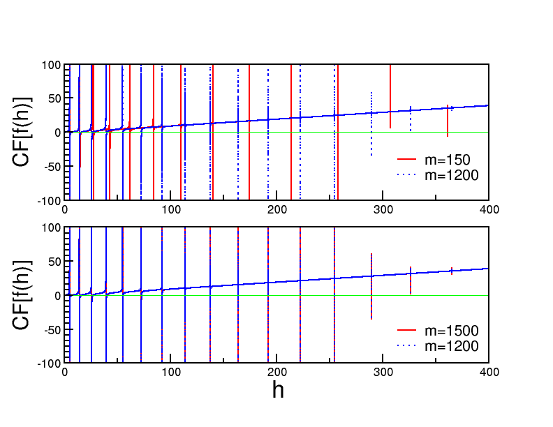
Figure 5: Plot of the continued fraction $CF[f(h)]$ for $n=10$ spikes. In the upper figure the red curve is for $m=150$ and the blue is for $m=1200$. In the lower figure the red curve is for $m=1500$ and the blue one is for $m=1200$.

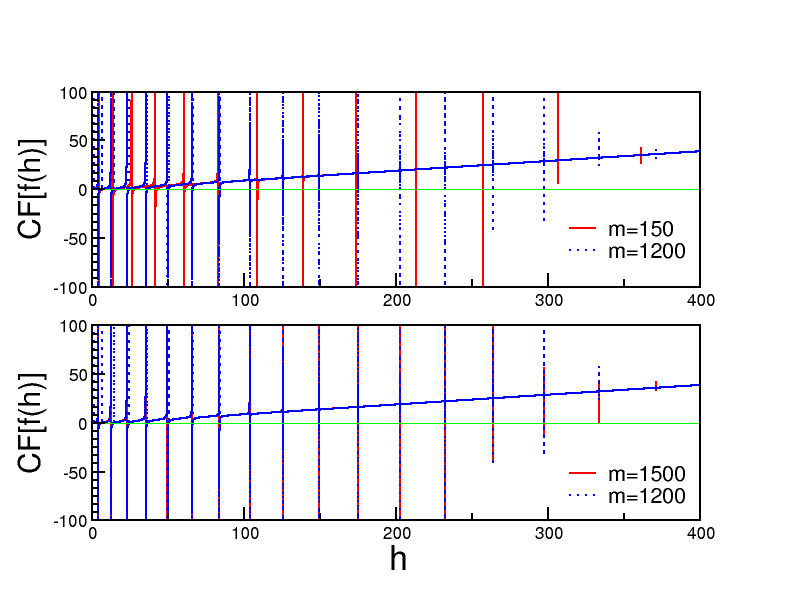
Figure 6: Plot of the continued fraction $CF[f(h)]$ for $n=3$ spikes. In the upper figure the red curve is for $m=150$ and the blue is for $m=1200$. In the lower figure, the red curve is for $m=1500$ and the blue one is for $m=1200$.

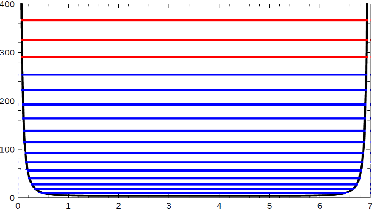
Figure 7: Plot of different roots in the potential $V(u)$ for $n=10$ spikes. The top three levels which we have used in our calculations, starting from top have $h=366.6$ (red), $h=326$ (red) & $h=290.2$ (red) respectively.

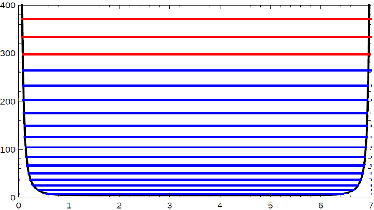
Figure 8: Plot of different roots in the potential $V(u)$ for $n=3$ spikes. The top three levels which we have used in our calculations, starting from top have $h=370.74$ (red), $h=333.23$ (red) & $h=297.87$ (red) respectively.

We solve the continued fraction numerically by using double precision. Figure (6) shows the plot of the continued fraction for two different $m$, $m=150$ (shown by a red curve) and $m=1200$ (shown by a blue curve). The $h$ values at which the graph intersects the $h$ axis, provides us with the roots. In Figure (6) one can see that there is some mismatch between the roots of the $m=150$ order truncation and $m=1200$ order truncation of the continued fraction. One can observe this by noting that the red curve and the blue curve cut the axis at different points. A convergence to the roots of the infinite continued fraction is reached when there is no mismatch between two truncations at different orders. Or, in other words we can say that if one considers two separate polynomials of $h$ of different orders and finds that the roots for the two different polynomials are very close in value to each other, then there is convergence. However, in the above example we can see that there is a mismatch and the values found with a truncation at a lower order (i.e at $m=150$) cannot be reliable . It is therefore certain from the above figure that to achieve convergence one has to truncate the infinite continued fraction at sufficiently higher order. Figure (6) shows the truncated continued fraction for $m=1200$ and $m=1500$. It is clear that there is almost no such mismatch as observed in Figure (6). The blue curves ($m=1200$) and the red curves ($m=1500$) overlap completely at least up to some finite domain of $h$. If one truncates at further higher order, the convergence will be even better.

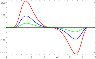
(a) Plot for $n=10$ with $h=366.6$ (red), $h=326$ (blue), & $h=290.2$ (green)

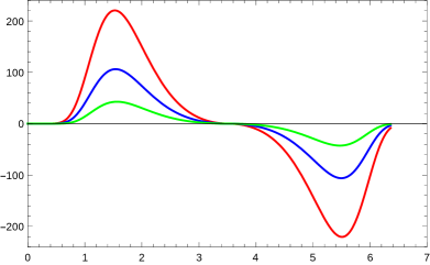
(b) Plot for $n=3$ with $h=370.74$ (red), $h=333.23$ (blue) , & $h=297.87$ (green)

Figure 9: Plot of $\delta t$ for $n=10~{}\&~{}3$ spikes for different $h$

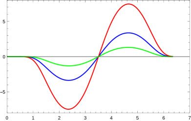
(a) Plot for $n=10$ with $h=366.6$ (red), $h=326$ (blue) , & $h=290.2$ (green)

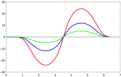
(b) Plot for $n=3$ with $h=370.74$ (red), $h=333.23$ (blue) , & $h=297.87$ (green)

Figure 10: Plot of $\delta\rho$ for $n=10~{}\&~{}3$ spikes for different $h$

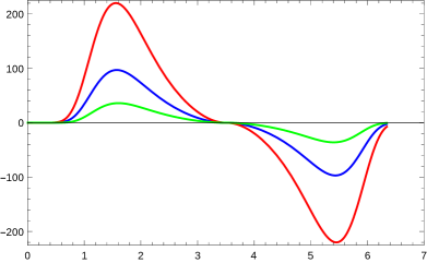
(a) Plot for $n=10$ with $h=366.6$ (red), $h=326$ (blue) , & $h=290.2$ (green)

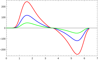
(b) Plot for $n=3$ with $h=370.74$ (red), $h=333.23$ (blue) , & $h=297.87$ (green)

Figure 11: Plot of $\delta\theta$ for $n=10~{}\&~{}3$ spikes for different $h$

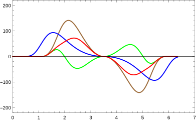
Figure 12: Plot of $\delta t$ for $h=326$ for four different number of terms i) $N=5$ (blue), ii) $N=21$ (brown), iii) $N=33$ (green) & iv) $N=43$ (red)

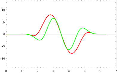
Figure 13: Plot of $\delta\rho$ for two negative ranges, $N$ = 33 (red) & $N$ = 73 (green).

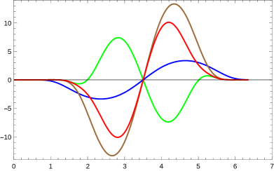
Figure 14: Plot of $\delta\rho$ for $h=326$ for four different number of terms i) $N=5$ (blue), ii) $N=21$ (brown), iii) $N=33$ (green) & iv) $N=43$ (red)

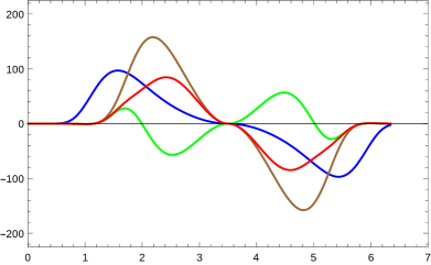
Figure 15: Plot of $\delta\theta$ for $h=326$ for four different number of terms i) $N=5$ (blue), ii) $N=21$ (brown), iii) $N=33$ (green) & iv) $N=43$ (red)

We now select three of the roots (eigenvalues), $h=366.6,~{}326,~{}\&~{}290.2$ for $n$ = 10 and $h=370.74,~{}333.23~{}\&~{}297.87$ for $n$ = 3 for which we compute the eigenstates and then, the perturbations, respectively. In Figures (8) and (8) we have shown the potential function for $n=10$ and $n=3$ spikes respectively. In our discussion later we will be working with the top three eigenvalues indicated by red lines. We show some of the eigenvalues and other parameters for spiky strings with $n=10$ and $n=3$ spikes in the table (1).

Table 1: Values of the parameters and eigenvalues for two different cases

$n$	$k$	$\alpha$	$\rho_{1}$	$\rho_{0}$	$h$
					$9.74,~{}18.09,~{}27.53,~{}40.07$
					$55.68,~{}72.95,~{}92.7,~{}114.41$
$10$	$0.985264$	$1.00914$	$3.18$	$1.068$	$-$
					$-$
					${\bf 290.2},~{}{\bf 326},~{}{\bf 366.6}$
					$-$
					$7.50,~{}15.23,~{}24.58,~{}36.65$
					$49.91,~{}66.12,~{}84.07,~{}103.97$
$3$	$0.985653$	$1.01232$	$2.645$	$0.45$	$-$
					$-$
					${\bf 297.87},~{}\bf{333.23},~{}\bf{370.74}$
					$-$

Let us now write down the general form of the perturbations. For the $\tau$ part of the solution we take only the real part i.e $\cos\beta\tau$. So the general form of the perturbations are

$$\begin{split}\delta t&=\phi n^{0}=\frac{\epsilon~{}\omega~{}\cos\beta\tau~{}\sqrt{\delta~{}\gamma~{}{\rm sn}^{2}(u,k)-2\delta~{}(\delta+1)+\frac{\eta~{}\delta}{{\rm sn}^{2}(u,k)}}}{\alpha-\gamma~{}{\rm sn}^{2}(u,k)}~{}{\rm sn}^{2}(u,k)~{}{\rm cn}(u,k)\\ &~{}{\rm dn}(u,k)\sum_{m=0}^{\infty}C_{m}~{}{\rm sn}^{2m}(u,k)\,\,,\end{split}$$ (47)

$$\begin{split}\delta\rho&=\phi n^{1}=\frac{-\epsilon~{}\cos\beta\tau~{}\sinh 2\rho_{0}}{\sqrt{\gamma^{2}~{}{\rm sn}^{4}(u,k)-2\gamma~{}(\delta+1)~{}{\rm sn}^{2}(u,k)+\alpha~{}\delta}}~{}{\rm sn}^{2}(u,k)~{}{\rm cn}(u,k)~{}{\rm dn}(u,k)\\ &\sum_{m=0}^{\infty}C_{m}~{}{\rm sn}^{2m}(u,k)\,\,,\end{split}$$ (48)

$$\begin{split}\delta\theta&=\phi n^{2}=\frac{\epsilon~{}\cos\beta\tau~{}\sqrt{\delta~{}\gamma~{}{\rm sn}^{2}(u,k)-2\delta~{}(\delta+1)+\frac{\eta~{}\delta}{{\rm sn}^{2}(u,k)}}}{\delta-\gamma~{}{\rm sn}^{2}(u,k)}~{}{\rm sn}^{2}(u,k)~{}{\rm cn}(u,k)~{}{\rm dn}(u,k)\\ &\sum_{m=0}^{\infty}C_{m}~{}{\rm sn}^{2m}(u,k)\,\,,\end{split}$$ (49)

where the coefficients $C_{m}$ for different cases are shown in the table (2).

Table 2: Values of the coefficients $C_{m}$ (Eqn. 38) for different cases

$n$	$h$	$\beta$	$C_{m}$
	290.2	$17.2$	$C_{0}=1,~{}C_{1}=-28.03,~{}C_{2}=248.6,~{}C_{3}=-910.09,$
			$C_{4}=1259.1,~{}C_{5}=95.33,~{}C_{6}=-952.5,~{}C_{7}=-657.46,......$
10	326	$18.22$	$C_{0}=1,~{}C_{1}=-31.61,~{}C_{2}=320.84,~{}C_{3}=-1390.1,$
			$C_{4}=2529.63,~{}C_{5}=-829.16,~{}C_{6}=-1947.05,~{}C_{7}=-236.62,.....$
	366.6	19.32	$C_{0}=1,~{}C_{1}=-35.67,~{}C_{2}=413.83,~{}C_{3}=-2107.39,$
			$C_{4}=4857.61,~{}C_{5}=-3524.75,~{}C_{6}=-2934.99,~{}C_{7}=1953.34,......$
	297.87	17.47	$C_{0}=1,~{}C_{1}=-28.8,~{}C_{2}=263.29,~{}C_{3}=-1001.62,$
			$C_{4}=1479.39,~{}C_{5}=-23.72,~{}C_{6}=-1145.42,~{}C_{7}=-644.47,.......$
3	333.23	18.48	$C_{0}=1,~{}C_{1}=-32.34,~{}C_{2}=336.51,~{}C_{3}=-1503.37,$
			$C_{4}=2865.34,~{}C_{5}=-1148.35,~{}C_{6}=-2160.91,~{}C_{7}=-16.34,......$
	370.74	19.49	$C_{0}=1,~{}C_{1}=-36.09,~{}C_{2}=423.95,~{}C_{3}=-2191.42,$
			$C_{4}=5157.14,~{}C_{5}=-3935.43,~{}C_{6}=-2986.85,~{}C_{7}=2317.27,......$

Figures (9), (10) & (11) show perturbations $\delta t,~{}\delta\rho,~{}\&~{}\delta\theta$ respectively for $n$ = 10 & $n$ = 3 spikes and each for three different roots ($h$) i.e $h=366.6,~{}326~{}\&~{}290.2$ for $n$ = 10 & $h=370.74,~{}333.23~{}\&~{}297.87$ for $n$ = 3 at constant $\tau$ (here $\tau=0$) and we find that all perturbations are finite and oscillatory in nature. Thus, it is now clear that the solution of the DTV equation which we have used leads to finite perturbations and therefore guarantees the stability of the spiky strings. The stability is however apparent even without writing down the above expressions explicitly. From the series solution given in Eqn.(38), the subsequent theorems which involves positive powers of ${\rm sn}(u,k)$ and the expressions for the normal components stated earlier, the finiteness of perturbations can indeed be qualitatively inferred.

3.3.1 Comments regarding the convergence issue

Recall from the previous section that we have obtained the eigenfunctions by truncating the infinite series involving powers of ${\rm sn}(u,k)$. Does the nature of the eigenfunctions change if we include more terms in the series. It is necessary to check this aspect though it is not really related to the qualitative behaviour and finiteness of the solutions which is our primary concern here.

Let us now address this convergence issue by considering more number of terms in the power series and observe the changes in the behaviour of the eigensolutions. Figures (13), (15) & (15) represent the perturbations $\delta t,~{}\delta\rho~{}\&~{}\delta\theta$ respectively for $h=326$ and for four different cases: 1) effect of inclusion of the first five terms in the series shown in blue curve, 2) effect of including the first 21 terms of the series shown in the brown curve, 3) effect of including the first 33 terms represented by the green curve and 4) effect of including the first 43 terms represented by the red curve. Here one observes some interesting features. Inclusion of up to the first 21 terms does not quite change the qualitative nature of the curve. However, when we begin adding more terms its nature does gradually change and after including 33 terms the curve flips completely, as shown in the green curve. Thereafter, if one keeps adding more number of terms in the series, we find that after adding 43 terms another overall sign flip occurs. The reason behind this flip can be easily found by considering the nature of the coefficients of the power series. We note that in the power series, the negative and positive terms alternate at the beginning (i.e. for the first few terms). Thereafter the inclusion of terms till a certain order yields only positive terms. Subsequently, we have negative terms up to a further order. This behaviour seems to repeat as we go on including more and more terms. When one considers first 33 terms one can find that there are sufficiently large number of negative coefficients so there is the flip in the curve. Similarly when one considers 43 terms, one can see there are sufficiently large number of positive terms and there is another flip of sign. Since this flipping occurs because of the alternating negativity or positivity of the coefficients one can ask which of two behaviours will eventually dominate if one includes sufficiently large number (ideally infinite) of terms.

Let us first check the case of negativity. Consider terms till the end of first set of negative values of the coefficients (i.e just before the set of positive coefficients begin). Thereafter, consider terms till the end of second set of negative values of the coefficients. A plot of the abovementioned two cases is shown in Figure (13) where the red curve represents the inclusions of 33 terms and the green curve includes 73 terms. One can easily see from Figure (13) that the amplitude of red curve is greater than the green one. Thus, one can say that the negativity effect is gradually diminishing. We have checked this by considering the inclusion of terms of very high orders and have found that the amplitudes of the negativity does indeed become smaller and smaller as more and more terms are included. It is therefore safe to state that when a very large number of terms are included the positive valued coefficients will dominate in the sum. This leads us to state that the nature of the perturbations will be very close to the curve represented in red in the Figure (13). Hence the graphs shown earlier representing the perturbations do reflect the qualitative nature of the perturbations correctly, though there will be quantitative differences (i.e in the exact values). Since our goal is to demonstrate that we have finite and oscillatory perturbations which imply the stability of the string configuration, we believe that it is not too crucial to be worried about exact numbers and values here.

4 Concluding remarks

In this article, which is a follow-up on our previous work [25], we have demonstrated that the spiky string solutions in three dimensional anti-de Sitter spacetime are stable against small deformations. Using the Jevicki-Jin embedding, we were able to reduce the perturbation equation to an equation known in the literature as the Darboux-Treibich-Verdier (DTV) equation. Thereafter, we used the solution of the DTV equation as stated in [36]. This solution involves an infinite series given in terms of the squares of the Jacobi sine elliptic functions. The eigenvalues are hidden in infinite continued fractions. By numerically solving the infinite continued fractions, we obtain the eigenvalues and the eigenfunctions. As shown in the previous section, the convergence of our solutions has been tested explicitly. Subsequently, we constructed the deformations $\delta x^{i}$ and through plots, we have shown that for the given eigenvalues the perturbations never diverge. We have checked our results for several eigenvalues. Thus, we can safely conclude that the spiky string solutions are indeed stable. The perturbations (for specific eigenvalues), as obtained in our work, may also be used to study the normal mode fluctuations of the spiky string worldsheet embedded in $AdS_{3}$. Unlike our previous work, where we dealt with spiky strings in flat spacetime (which do not have any link with AdS/CFT), here, it would certainly be interesting to understand the role of the perturbations, in relation to the AdS/CFT correspondence. Furthermore, generalisations to higher dimensional AdS backgrounds and a study of perturbations of the string configurations therein will be of interest in future work. The spectrum of perturbations may also be linked to the computation of quantum corrections [37] in some way. Finally, as an aside, the eigenvalues and eigenfunctions of the special case of the DTV equation, which we have obtained by solving the continued fraction numerically can be explored in the context of an analog quantum mechanics problem with a DTV potential, as well as its periodic generalisations. We hope to return to such issues in future.

References

- [1] C. J. Burden and L. J. Tassie, “Some exotic mesons and glueballs from the string model,” Phys. Letts. B 110, 64 (1982).
- [2] C. J. Burden and L. J. Tassie, “Rotating strings, glueballs and exotic mesons,” Aust. Jr. Phys. 35, 223 (1982).
- [3] C. J. Burden and L. J. Tassie, “ Additional rigidly rotating solutions in the string model of hadrons,” Aust. Jr. Phys. 37, 1 (1984).
- [4] C. J. Burden, “Gravitational radiation from a particular class of cosmic strings,” Phys. Letts. B, 164, 277 (1985).
- [5] F. Embacher, “Rigidly rotating cosmic strings,” Phys. Rev. D 46, 3659 (1992); Erratum Phys. Rev. D 47, 4803 (1993).
- [6] H. de Vega and I. L. Egusquiza, “ Planetoid string solutions in axisymmetric spacetimes”, Phys. Rev. D 54, 7513 (1996) [arXiv:hep-th/9607056].
- [7] V. Frolov, S. Hendy and J. P. de Villiers, “ Rigidly rotating strings in stationary axisymmetric spacetimes”, Class. Qtm. Grav. 14, 1099 (1997) [arXiv:hep-th/9612199].
- [8] S. Kar and S. Mahapatra, “ Planetoid strings: solutions and perturbations”, Class. Qtm. Grav. 15, 1421 (1998) [arXiv:hep-th/9701173].
- [9] C. J. Burden, “Comment on “Stationary rotating strings as relativistic particle mechanics”,” Phys. Rev. D 78, 128301 (2008).
- [10] K. Ogawa, H. Ishihara, H. Kozaki, H. Nakano and S. Saito, “ Stationary rotating strings as relativistic particle mechanics ”, Phys. Rev. D 78, 023525 (2008) [arXiv:gr-qc/0803.4072].
- [11] J. M. Maldacena, “The Large N limit of superconformal field theories and supergravity,” Int. J. Theor. Phys. 38, 1113 (1999) [Adv. Theor. Math. Phys. 2, 231 (1998)] [hep-th/9711200].
- [12] M. Kruczenski, “Spiky strings and single trace operators in gauge theories,” JHEP 0508, 014 (2005) [arXiv:hep-th/0410226].
- [13] S. S. Gubser, I. R. Klebanov and A. M. Polyakov, Nucl. Phys. B 636, 99 (2002) [hep-th/0204051].
- [14] J. A. Minahan and K. Zarembo, “The Bethe ansatz for =4 super Yang-Mills,” JHEP 0303, 013 (2003) [hep-th/0212208].
- [15] L. Dolan, C. R. Nappi and E. Witten, “A Relation between approaches to integrability in superconformal Yang-Mills theory,” JHEP 0310, 017 (2003) [arXiv:hep-th/0308089].
- [16] L. Dolan, C. R. Nappi and E. Witten, “Yangian symmetry in superconformal Yang-Mills theory,” [arXiv:hep-th/0401243]
- [17] G. Mandal, N. V. Suryanarayana and S. R. Wadia, “Aspects of semiclassical strings in AdS(5),” Phys. Lett. B 543, 81 (2002) [hep-th/0206103].
- [18] I. Bena, J. Polchinski and R. Roiban, “Hidden symmetries of the AdS(5) x S**5 superstring,” Phys. Rev. D 69, 046002 (2004) [hep-th/0305116].
- [19] S. Frolov and A. A. Tseytlin, “Multispin string solutions in AdS(5) x S**5,” Nucl. Phys. B 668, 77 (2003) [hep-th/0304255].
- [20] R. Ishizeki and M. Kruczenski, “Single spike solutions for strings on and ,” Phys. Rev. D 76, 126006 (2007) [arXiv:0705.2429 [hep-th]].
- [21] R. Ishizeki, M. Kruczenski, A. Tirziu and A. A. Tseytlin, “Spiky strings in and their AdS-pp-wave limits,” Phys. Rev. D 79, 026006 (2009) [arXiv:0812.2431 [hep-th]].
- [22] S. Biswas and K. L. Panigrahi, “Spiky Strings on I-brane,” JHEP 1208, 044 (2012) [arXiv:1206.2539 [hep-th]].
- [23] A. Banerjee, K. L. Panigrahi and P. M. Pradhan, “Spiky strings on with NS-NS flux,” Phys. Rev. D 90, no. 10, 106006 (2014) [arXiv:1405.5497 [hep-th]].
- [24] A. Banerjee, S. Bhattacharya and K. L. Panigrahi, “Spiky strings in -deformed ,” JHEP 1506, 057 (2015) [arXiv:1503.07447 [hep-th]].
- [25] S. Bhattacharya, S. Kar and K. L. Panigrahi, “Perturbations of spiky strings in flat spacetimes”, JHEP 01, 116 (2017) [arXiv:hep-th/1610.09180].
- [26] S. Frolov and A. A. Tseytlin, “Semiclassical quantization of rotating superstring in AdS(5) x S**5,” JHEP 0206, 007 (2002) [hep-th/0204226].
- [27] J. Garriga and A. Vilenkin, “Black holes from nucleating strings,” Phys. Rev. D 47 3265 (1993) [arXiv:hep-ph/9208212].
- [28] J. Guven, “Perturbations of a topological defect as a theory of coupled scalar fields in curved space interacting with an external vector potential,” Phys. Rev. D 48, 5562 (1993) [arXiv:gr-qc/9304033].
- [29] V. Frolov and A. L. Larsen, “Propagation of perturbations along strings”, Nucl. Phys. B 414, 129 (1994) [arXiv:hep-th/9303001].
- [30] R. Capovilla and J. Guven, “Geometry of deformations of relativistic membranes,” Phys. Rev. D 51, 6736 (1995) [arXiv:gr-qc/9411060].
- [31] V. Forini, V. Giangreco, M. Puletti, L. Griguolo, D. Seminara, E. Vescovi, “Remarks on the geometrical properties of semiclassically quantized strings”, J. Phys A: Math. Theor., 48, 475401 (2015) [arXiv:1507.01883 [hep-th]].
- [32] A. Jevicki and K. Jin, “Solitons and AdS string solutions”, Int. Jr. Mod. Phys. A 23, 2289 (2008) [arXiv:0804.0412 [hep-th]].
- [33] Comte de Sparre, “ Sur l’equation….” Acta Mathematica 3, 105–140 (1883).
- [34] Comte de Sparre, “ Sur l’equation….” Acta Mathematica 3, 289–321 (1883).
- [35] V. B. Matveev and A. O. Smirnov, “On the Link Between the Sparre Equation and Darboux-Treibich-Verdier Equation”, Lett. Math. Phys. 76, 283 (2006).
- [36] Y-M. Chiang, A. Ching and C-Y. Tsang, “Symmetries of the Darboux equation”, [arXiv:1509.03995 [math]] (to appear in Kumamoto Journal of Mathematics).
- [37] S. Frolov, A. Tirziu and A. A. Tseytlin, “Logarithmic corrections to higher twist scaling at strong coupling from AdS/CFT”, Nucl. Phys. B 766, 232 (2007) [arXiv:hep-th/0611269].