Spontanous spin squezing in a rubidium BEC

Abstract

We describe an experiment where spin squeezing occurs spontaneously within a standard Ramsey sequence driving a two-component Bose-Einstein condensate (BEC) of ⁸⁷Rb atoms trapped in an elongated magnetic trap. Multiparticle entanglement is generated by state-dependent collisional interactions, despite the near-identical scattering lengths of the spin states in ⁸⁷Rb. In our proof-of-principle experiment, we observe a metrological spin squeezing that reaches $1.3\pm 0.4\,$dB for $5000$ atoms, with a contrast of $90\pm 1$%. The method may be applied to realize spin-squeezed BEC sources for atom interferometry without the need for cavities, state-dependent potentials or Feshbach resonances.

Introduction

Bose-Einstein condensates (BECs) of atoms with more than one spin state present rich dynamics in their spin and motional degrees of freedom. Most experiments so far have focused on either spin or real-space evolution, carefully avoiding time-dependent evolution in the other subspace. One class of experiments prepares each atom in the BEC in a precisely controlled spin superposition and explores the complex spatial phase dynamics that deploys due to the spin-dependent interactions [1]. In these studies, mainly focused on the mean field dynamics, the spin state remains unchanged throughout the evolution. Other experiments, by contrast, use the condensed sample as a support for spin dynamics, especially to generate entangled spin states, while spatial dynamics is carefully avoided [2, 3]. Only a few recent experiments have started to explore the interplay of spatial and spin dynamics in order to generate different forms of entanglement in two-component or spinor BECs [4, 5, 6], including spin squeezing. Spin-squeezed states [7, 8] are the prime example of highly entangled many-particle states with the potential to improve atomic clocks and interferometric sensors beyond the standard quantum limit [9]. This metrological prospect also applies to BECs which, due to their minimum phase-space spread, are considered as precious source states for atom interferometry [9, 10, 11] despite their inherent fluctuations, phase diffusion and losses. Furthermore, the spin squeezing parameter can be used to quantify the degree of entanglement between the condensate atoms [12]. For all these reasons, spin-squeezed states of BECs have met with wide interest, and it has been pointed out early on that such states can naturally arise in two-component BECs due to different scattering lengths between the internal states [12]. Yet, experiments with two-component BECs have not produced such states, except when atomic interactions were enhanced with the help of a Feshbach resonance [3] or by actively separating the spin components in a state-dependent trap [4]. Both methods have led to spectacular results, but come at the price of a considerably more complex setup. Here we describe an experiment where spin squeezing occurs spontaneously after an internal state quench, the dynamics being initiated simply by an initial $\pi/2$ pulse [13] applied to a rubidium BEC in a harmonic trap.

1 Origin of spontaneous spin squeezing

The basic idea of creating spin squeezing by atomic interaction in a BEC, as originally envisaged in 2001 [12], is easily understood in the basis of well-defined atom numbers $\left|N_{1}\right\rangle$ and $\left|N_{2}\right\rangle$=$\left|N-N_{1}\right\rangle$, where the index refers to the spin state and $N$ is the total atom number, which we consider fixed for now. On the $N$-atom Bloch sphere, each state with a given $N_{1}$ corresponds to a circle of fixed latitude. If the energy of these states depends monotonically on $N_{1}$, a superposition of several $\left|N_{1}\right\rangle$, such as a coherent state, will not evolve with constant phase speed on the Bloch sphere, but will be sheared. This leads to spin squeezing due to the well-known “one-axis twisting” Hamiltonian [7]. More precisely, for a BEC with spin states $i=1,2$ having spatial wavefunctions $\phi_{i}(\mathbf{r})$, and $S_{z}=(N_{2}-N_{1})/2$, the spin interaction can be written

$$H_{\text{int}}/\hbar=\chi S_{z}^{2}\,.$$ (1)

Neglecting the dependence of the condensate mode on atom number, $\chi$ can be written simply [14].

$$\chi=(U_{11}+U_{22}-2U_{12})/(2\hbar)\qquad\mbox{and}\qquad U_{jk}=g_{jk}\int dr^{3}|\phi_{j}|^{2}|\phi_{k}|^{2}$$ (2)

with $g_{jk}=4\pi\hbar^{2}a_{jk}/m$ and $m$ the mass of the atom. Significant squeezing develops for times $t$ such that $\chi t\geq\frac{1}{N}$ [16]. However, when all scattering lengths are nearly equal, $a_{11}\approx a_{22}\approx a_{12}$ as in the case of ⁸⁷Rb, and there is full spatial overlap between the components, population imbalance causes only a small energy change, and $\chi$ becomes so small that the required $t$ is unrealistically large. This rules out the straightforward implementation of BEC squeezing in ⁸⁷Rb – the most widely used atom in two-component BEC experiments and in cold-atom metrology today. If, on the other hand, the overlap of the components is reduced, then a sizeable nonlinear interaction exists even for identical scattering lengths [4, 17, 13].

Under properly chosen trapping conditions, spatial dynamics of the spin components will occur spontaneously [18], reducing the overlap and thus creating spin squeezing. Note that the spatial dynamics is created by the same difference of scattering lengths which, while too weak to create spin squeezing on its own, can be strong enough to drive the spatial separation which then causes the squeezing. $\chi$ dynamically increases during the separation, generating the squeezing, and then decreases again as the atoms oscillate back to their initial position.

In this article, we experimentally demonstrate this effect. In our experiment, an elongated trap is operated near the “magic” bias field [19, 20] where trapping frequencies are identical for two hyperfine ground state sublevels $\left|1\right\rangle\equiv\left|F=1,m_{F}=-1\right\rangle$ and $\left|2\right\rangle\equiv\left|F=2,m_{F}=1\right\rangle$. The condensate is initially prepared in $\left|1\right\rangle$ and subjected to a $\pi/2$ pulse on the $\left|1\right\rangle\leftrightarrow\left|2\right\rangle$ transition. The subsequent free evolution in the cigar-shaped trap leads to demixing of the two components [21, 18, 22, 13, 23], initiating the squeezing dynamics (Fig. 1). By applying a second pulse to close the spin interferometer when the $\left|1\right\rangle$ component oscillates back into overlap with $\left|2\right\rangle$, we indeed observe not only a contrast revival, but also a simultaneous reduction of spin projection noise, yielding metrological spin squeezing.

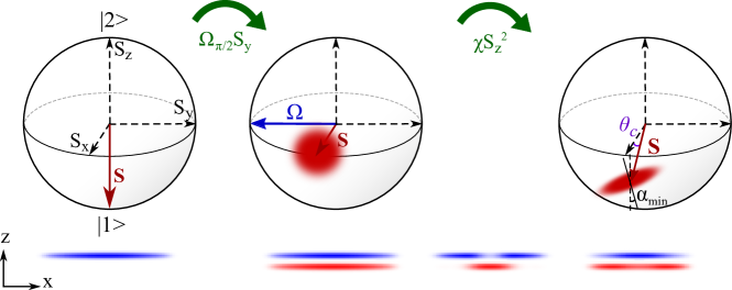
Figure 1: Experimental sequence. A first $\pi/2$ pulse of Rabi frequency $\Omega$ places the condensate in a coherent superposition. This initiates state-dependent spatial dynamics, leading to the shearing of the spin noise distribution. Due to asymmetric losses, the mean spin is also tilted below the equatorial plane by an angle $\theta_{c}$. A second pulse of variable duration is applied in order to rotate the spin distribution before detecting the atom numbers $N_{1}$ and $N_{2}$. The clouds below the Bloch spheres represent the spatial dynamics undergone by the two states $\left|1\right\rangle$ (blue) and $\left|2\right\rangle$ (red).

2 Experiment

The experiment is performed on the Trapped-Atom Clock on a Chip (TACC) platform, described in detail in [24, 25, 20]. In contrast to those references, here we use a BEC. An atom chip generates the magnetic field gradients for trapping and also carries the two-photon, radiofrequency (RF) and microwave (MW) signals for exciting the clock transition. Atoms are initially trapped in $\left|1\right\rangle$ and cooled by forced RF evaporation in a tight trap. We continue the RF ramp well into the BEC regime, obtaining condensates with no discernible thermal fraction and containing up to $\sim 14000$ atoms. The magnetic potential is then slowly (600 ms) transformed into an interrogation trap with frequencies $\omega_{x,y,z}=2\pi\times(2.7,92,74)\,\mbox{Hz}$ unless otherwise specified, located $z=350\,\mu$m below the chip surface ($z=0$). The lifetime of the BEC in this trap is about $5\,s$, limited by collisions with thermal atoms in the single vacuum cell. The atom number in this trap is controlled with the MOT loading time and the final frequency of the evaporation ramp.

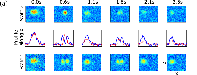
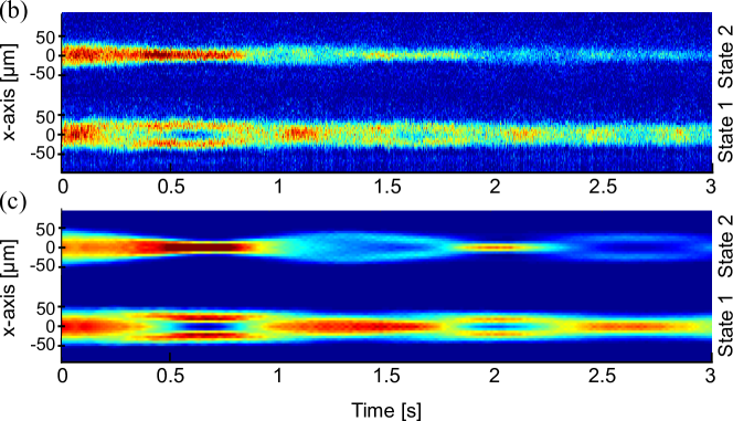
Figure 2: Spatial dynamics observed in absorption imaging after a 30 ms time of flight. Note that these images are taken with an auxiliary imaging system along the $y$ axis, which has higher noise than the one used for the squeezing measurements below. For these measurements, a BEC of $10^{4}$ atoms is produced in state $\left|1\right\rangle$ in a trap with trap frequencies $\omega_{x,y,z}=2\pi\times(2.7,92,74)\,\mbox{Hz}$. A resonant $\pi/2$ pulse prepares an equal superposition of $\left|1\right\rangle$ and $\left|2\right\rangle$ and the cloud dynamics are monitored in time. (a) Individual images taken after the evolution times indicated in the figure. (b) Many such images integrated along $z$ and assembled to show the spatial dynamics along $x$. (A common-mode sloshing that was present in this experiment has been subtracted.) (c) 3D coupled Gross-Pitaevskii numerical simulation for the atom numbers and trap frequencies of the experiment.

We use the $\left|1\right\rangle\leftrightarrow\left|2\right\rangle$ clock transition, which enables first-order cancellation of spatial inhomogeneity of the transition frequency in a magnetic trap [19, 26]. The transition is driven by a two-photon, RF and MW pulse [20] with Rabi frequency $\Omega=2\pi\times 3.6\,$Hz. The MW signal at 6.8 GHz is generated by a custom-built synthesizer [27], while the RF photon of $\approx 2\,$MHz comes from a commercial direct-digital synthesizer. Both are referenced to SYRTE’s active hydrogen maser [20]. After preparing a BEC in the interrogation trap, the sequence always starts by applying a resonant $\pi/2$ pulse to create the superposition $1/2^{N/2}(\left|1\right\rangle+\left|2\right\rangle)^{\otimes N}$ (see A). Due to the slight difference in scattering lengths, the initial density distribution no longer corresponds to a stationary state, and the two components start to oscillate [21, 18, 28, 29, 30, 23]. To reveal the resulting spatial dynamics, we have imaged both states using an auxiliary imaging system on the $y$ axis, so that the slow $x$ axis is visible. Images are taken at variable times after the pulse. A typical result is shown in Fig. 2. The $\left|1\right\rangle$ component splits into two parts which oscillate along the weak axis, while the $\left|2\right\rangle$ component does not separate but undergoes a breathing-type oscillation in the center between the $\left|1\right\rangle$ component’s two lobes. After a period of $1.2\,$s, the $\left|1\right\rangle$ component has come back into superposition with $\left|2\right\rangle$ and another oscillation begins. For longer times, a third oscillation is barely visible. A 3D numerical simulation using coupled Gross-Pitaevskii equations (GPEs) reproduces the features of the observed oscillation (Fig. 2(b)) reasonably well, however, the calculated and measured oscillation frequencies differ by 20 %. One possible reason for this difference could be a residual thermal cloud too weak to be visible on the camera images.

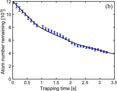
Figure 3: Atom number as a function of trapping time in the interrogation trap for condensates with all atoms in $\left|1\right\rangle$ (cyan squares), all atoms in $\left|2\right\rangle$ (magenta stars) and with atoms in an equal superposition (blue diamonds: $N_{1}$, red circles: $N_{2}$). The fit to the $\left|1\right\rangle$ data is a simple exponential, yielding the $5$ s background-limited lifetime. The other lines are not fits, but predictions without adjustable parameters, using published values [30] for the two-body decay rates, $\gamma_{22}=8.1(3)\times 10^{-14}\mbox{cm}^{3}/\mbox{s}$ and $\gamma_{12}=1.51(18)\times 10^{-14}\mbox{cm}^{3}/\mbox{s}$, and our experimentally determined densities. The latter are obtained from the measured atom numbers and the trap frequencies, assuming a BEC in the dimensional crossover regime. (b) Total atom number $N_{1}+N_{2}$ as a function of time, starting from an initial atom number $N\sim 1.2\times 10^{4}$ in equal superposition of $\left|1\right\rangle$ and $\left|2\right\rangle$. The blue points are experimental data, while the solid line has been obtained by numerical integration of coupled GPEs.

While these images are instructive for observing the spatial dynamics, measurements of the atom numbers are better performed by imaging along the $x$ axis, where the cloud covers fewer pixels. We use saturated absorption imaging [31] and state-selective release from the trap so that both states can be detected in the same image with a back-illuminated deep depletion CCD with high quantum efficiency. The imaging system is carefully calibrated for absolute accuracy as described in A.

Density-dependent atom losses are an important limiting factor in BEC spin squeezing [3, 32]. While the background-limited lifetime of state $\left|1\right\rangle$ is much longer than the oscillation period, state $\left|2\right\rangle$ has additional loss channels which reduce its lifetime. To measure the relevant loss parameters, we prepare a BEC in $\left|1\right\rangle$, $\left|2\right\rangle$ or an equal superposition of both states, and measure the remaining populations in the interrogation trap after different trapping times. The results are displayed on Fig. 3 (points). An exponential fit to the $\left|1\right\rangle$ data yields a $5$ s background-limited lifetime. The other curves in Fig. 3(a) are not fits but predictions without adjustable parameters as described in the caption. They reproduce the data well, as does the simulation using coupled GPEs (Fig. 3(b)). In our experiments, number densities in the $\left|2\right\rangle$ state range from $1\times 10^{12}$ to $8\times 10^{12}\,\mbox{cm}^{-3}$, corresponding to two-body loss limited lifetimes ranging from $12\,$s to as short as $1.5\,$s, respectively. In the following, $N_{\text{i}}$ refers to the initial atom number and $N_{\text{f}}$ to the atom number measured at the end of the experimental sequence.

3 Oscillation of the Ramsey contrast

Because the oscillation puts the atoms into motion and changes the spatial overlap of the components, it also manifests itself in the contrast of the Ramsey fringes when a second $\pi/2$ pulse is added after a time $T_{R}$. Fig. 4(a) shows the evolution of this contrast (red circles) as a function of $T_{R}$ for $N_{\text{i}}=1.2\times 10^{4}$. For this atom number, the initial contrast of 98% drops to about 50% around 600 ms, and then shows a revival at $T_{R}=1.2\,$s , which reflects the spatial overlap between the two modes at this time. Indeed, we find that the contrast revival time coincides with the spatial oscillation period observed by absorption imaging. This period depends on trap frequencies and atom number [30].

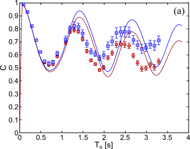
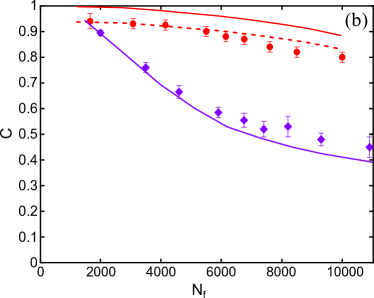
Figure 4: Contrast of a Ramsey measurement consisting of two $\pi/2$ pulses separated in time by $T_{R}$, performed in the interrogation trap with frequencies $\omega_{x,y,z}=2\pi\times(2.7,92,74)\,\mbox{Hz}$. For each $T_{R}$, the frequency of the two pulses is scanned around resonance to measure the fringe contrast $C$, defined by a fit according to $P_{2}=\frac{1}{2}(1+C\text{cos}(2\pi\Delta\nu T_{R}+\varphi_{lo}))$, where $P_{2}=N_{2}/N_{\text{f}}$, $T_{R}$ is the Ramsey time and corresponds to the time during which the interferometer is sensitive to phase variations, and $\Delta\nu$ is the detuning from atomic resonance. (a) Measured contrast (red circles), corrected contrast (blue squares) and corresponding predictions of the coupled GPE simulation (solid lines), as a function of Ramsey time for $N_{\text{i}}=1.2\times 10^{4}$. (b) Corrected contrast at the revival time (red circles) and half the revival time (purple diamonds) as a function of $N_{\text{f}}$. The corresponding solid lines are results of the GPE simulations. The dashed line shows the simulation result multiplied with a decoherence term (exponential decay) which accounts for decoherence sources not contained in the simulation. Its value $\gamma_{d}=0.5s^{-1}$ is chosen to match the maximum experimental contrast.

Due to the state-dependent losses, the population imbalance is time-dependent. Right after the initial $\pi/2$ pulse, the polar angle of the Bloch vector is $\theta=\pi/2$, but then slowly evolves to a value $\theta=\pi/2+\theta_{c}$ at time $T_{R}$ (Fig. 1). To obtain maximum contrast (and thus, maximum phase sensitivity in the final measurement), $\theta_{c}$ must be taken into account. In an actual atomic clock or interferometer, this can be achieved by inserting a correction pulse with a well-defined phase before the second $\pi/2$ pulse to remove the known mean value $\bar{\theta}_{c}$. The contrast that one would get by applying such a correction pulse can also be derived numerically using simple geometric considerations (A). We have used both, correction pulses and numerical contrast correction, and find that the results are consistent. Unless otherwise indicated, the results below use the numerical correction method. Note that only the mean value of $\theta_{c}$ can be removed or corrected, while the noise introduced by the statistical nature of the losses remains and contributes to the final noise budget [3, 32]. We will come back to this point below.

The corrected contrast, represented by blue squares in Fig. 4(a), shows a first revival of 82% for $N_{\text{i}}=1.2\times 10^{4}$. The precise value of the contrast, and thus the spatial dynamics, also depends on atom number, as shown in Fig. 4(b). Lower atom numbers result in higher contrast revivals.

The numerical simulations described above qualitatively reproduce the observed time evolution and provide some additional insight (solid lines in Fig. 4). The contrast minimum occurring at half the revival time decays faster than the contrast maximum at the revival time. Its simulated value is in good agreement with the experiment, confirming that the decay is caused by a stronger spatial separation for higher atom numbers. Both the demixing period and the contrast at revival time are overestimated in the simulation, even though the population decay is well reproduced (cf. Fig. 3(b)). The lower revival contrast suggests experimental sources of decoherence that are not contained in the simulation. Indeed, multiplying with a decoherence term with $\gamma_{d}=0.5s^{-1}$ brings the simulated contrast into agreement with the measured values (dashed line in Fig. 4(b)). For the revival period, the source of the deviation is less obvious, one possible candidate being a dilute thermal cloud as mentioned above.

Note that the density-dependent frequency shift [19], combined with the spatial dynamics and atom losses, leads to a time dependence of the atomic transition frequency $\nu_{12}$: the resonance frequency of the pulse applied in the beginning of the sequence is slightly higher than that at the revival time. Although the shift is small (on the order of $-10^{-4}\,$Hz per atom for our trap), it is easily detected in a metrology setup like ours and needs to be taken into account in the squeezing measurements, as detailed below. In particular, for every atom number and Ramsey time, we use the adequate effective resonance frequency, which is determined in a separate measurement (see A).

4 Spin noise measurements

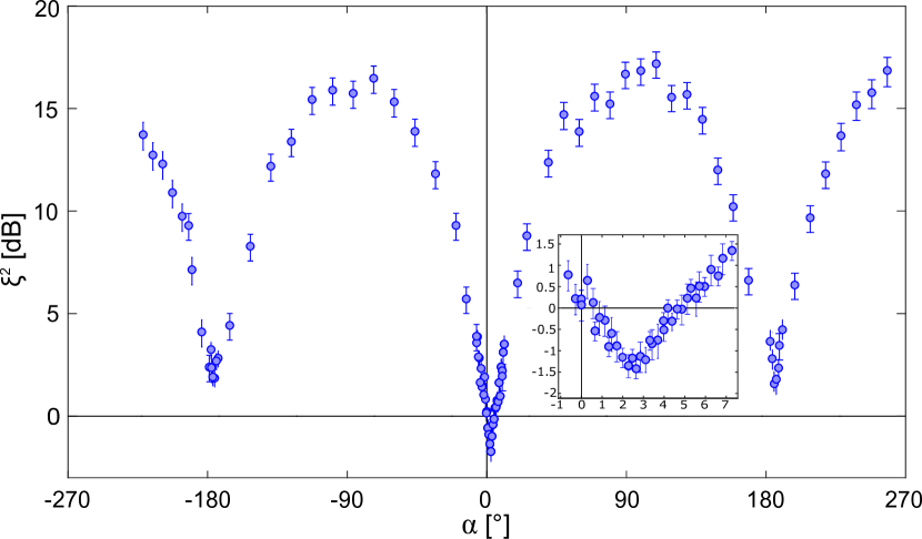
Figure 5: Measured spin noise for a final atom number $N_{\text{f}}\approx 5000$ and trap frequencies $\omega_{x,y,z}=2\pi\times(2.7,92,74)\,\mbox{Hz}$. The squeezing factor $\xi^{2}=\Delta_{n}S_{z}^{2}=4\Delta S_{z}^{2}/C^{2}\overline{N_{\text{f}}}$ is shown as a function of the tomography angle $\alpha$, with error bars corresponding to a 68$\%$ confidence interval. The inset is a zoom of the main plot in the region where $\xi^{2}$ reaches its minimum.

We use spin noise tomography to characterize the spin distribution that is generated in the dynamically evolving two-component BEC, . As before, a BEC with a precisely controlled atom number is produced in $\left|1\right\rangle$ and we apply a first near-resonant $\pi/2$ pulse which puts each atom into a coherent superposition between the two clock states. The BEC then evolves freely in the trap during a time $T_{R}$ which we adjust to coincide exactly with the contrast revival time measured above. During the free evolution, the spin distribution undergoes the nonlinear collisional interaction enhanced by the spatial separation of the two components. At the time $T_{R}$, a second pulse (“analysis pulse”) is used to rotate the spin distribution about its center, which has been determined separately (see Fig. 1 and A). By changing the duration of the analysis pulse, the rotation angle $\alpha$ (“tomography angle”) can be varied. After this rotation, the trap is switched off and the atom numbers $N_{1}$ and $N_{2}$ are measured. For each $\alpha$, the whole preparation and analysis sequence is repeated a large number of times (typically 300 repetitions) and the normalized population difference $S_{z}^{n}=\frac{1}{2}\frac{N_{2}-N_{1}}{N_{1}+N_{2}}$ is determined. The number squeezing $\mathcal{V}^{2}=\frac{4\Delta S_{z}^{2}}{\overline{N_{\text{f}}}\text{cos}(\overline{\theta_{c}})^{2}}$ and the squeezing factor $\xi^{2}=\frac{4\Delta S_{z}^{2}}{\overline{N_{\text{f}}}C^{2}\text{cos}(\overline{\theta_{c}})^{2}}$ [8] are then derived in order to quantify the spin noise reduction and the metrologically useful spin squeezing respectively, $\Delta S_{z}^{2}$ being the variance of the spin in the y-z plane (Fig. 1). The contrast is determined separately using the procedure detailed on Fig. 4. Fig. 5 shows the result for a final atom number $N_{\text{f}}\approx 5000$ and trap frequencies $\omega_{x,y,z}=2\pi\times(2.7,92,74)\,\mbox{Hz}$. As expected, the measured noise corresponds to a slightly tilted, ellipse-shaped distribution. The minimum squeezing factor occurs for an angle $\alpha=2.5^{\circ}$ and reaches $\xi^{2}=-1.3\pm 0.4$ dB with a contrast of 90$\pm$1$\%$ for this parameter set. It corresponds to atom number fluctuations of $\pm 32$ atoms for each component.

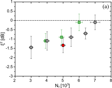
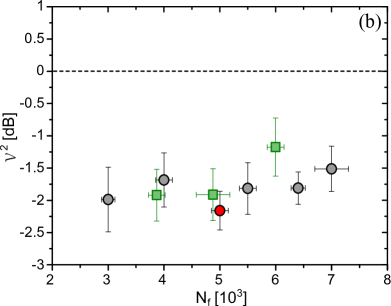
Figure 6: Squeezing factor (a) and number squeezing (b) as a function of the detected atom number for two different traps. Black circles: $\omega_{x,y,z}=2\pi\times(2.7,92,74)\,\mbox{Hz}$, green squares: $\omega_{x,y,z}=2\pi\times(4.4,128,113)\,\mbox{Hz}$. The red point corresponds to the data displayed on Fig. 5. The result for the stronger trap are generally worse in spite of the faster dynamics ($T_{R}=0.7$s). While the metrological squeezing factor deteriorates with increasing atom number, no clear tendency is visible in the number squeezing. This indicates that the squeezing factor is mostly limited by the contrast reduction occurring when increasing the atom number, as shown in Fig. 4 (b).

We have repeated these measurements for different atom numbers up to the maximum BEC atom number accessible in our experiment, and for a second, stronger trap with frequencies $\omega_{x,y,z}=2\pi\times(4.4,128,113)\,\mbox{Hz}$. The results are shown in Fig. 6. The squeezing factor $\xi$ deteriorates for $N_{\text{f}}>5000$, but seems to saturate for smaller $N_{\text{f}}$. Interestingly, the number fluctuations (Fig. 6(b)) do not show these tendencies, but maintain a constant level within the error bars. The deterioration of $\xi$ is mostly due to the reduced contrast at high atom numbers (Fig. 4(b)). Both effects will be discussed in the next section.

5 Limiting factors

The squeezing factor $\xi$ observed at the revival time results from the competition between the twisting interaction (eq. 1) and the state-dependent losses and non-perfect spatial revival dynamics: the latter two introduce new fluctuations and reduce contrast. The two main parameters that can be experimentally controlled are the atom number $N$ and the trap frequencies $\omega_{x,y,z}$. Higher atom numbers and higher trap frequencies increase the condensate density, which accelerates the squeezing dynamics by increasing $\chi$, but also accelerates the two-body losses. In the case of a homogeneous system or in separated harmonic traps for the two components, the two effects cancel [32, 16], so that one does not expect a density dependence of the squeezing factor $\xi$. In our case, the spatial dynamics lead to a significantly more complicated situation. $\chi$ as well as the contrast depend on the spatial overlap of the spin components, which is time-dependent (cf. Fig. 4) with an evolution that depends on $N$ as well as on $\omega_{x,y,z}$. The rather high value of the contrast at $T_{R}/2$ (Fig. 4) indicates that the component separation is not complete. For complete separation and our range of atom numbers, it is known that $\chi$ would be large enough to reduce number fluctuations by several orders of magnitude in a time much shorter than our revival time (see B), even when losses are taken into account. In the absence of losses, these high values could still be reached with incomplete separation, at the expense of a longer squeezing time. Thus, in our situation, the state-dependent losses (Fig. 3) clearly have a major effect on the final result. In an attempt to obtain more quantitative predictions, we have performed beyond-GPE simulations, described in the next section.

Apart from these fundamental contributions, technical noise such as phase noise can limit the measurement of the noise reduction induced by the squeezing process. In order to evaluate our system in terms of technical instabilities, a standard clock measurement, similar to the one conducted in [20], has been performed using the same experimental condition as for Fig. 5. This measurement yielded a fractional frequency stability of $9.7\times 10^{-12}\tau^{-1/2}$. Several noise sources have been investigated to explain this stability, and atom loss has been identified as the major contribution to the stability budget ($8.47\times 10^{-12}\tau^{-1/2}$). This is due to the fact that, for each shot, we only have access to the final populations. We therefore do not precisely know how many atoms have been lost during the sequence, nor when they were lost. For instance, if an atom is lost at the beginning of the Ramsey time, it will not contribute to the collisional shift, whereas if it is lost right before the second interrogation pulse, it was partly responsible for this frequency shift, but will not be detected. This leads to a noise on $S_{z}$ that we cannot correct. This noise also impacts the squeezing measurement, contributing on the order of 9% of the quantum projection noise. Subtracting this noise would bring $\xi^{2}$ from $-1.3\,$dB to $\xi^{2}\approx-2\,$dB: its contribution is non-neglegible, but it does not limit the order of magnitude of the observed squeezing.

6 Simulations beyond GPE

While the spatial dynamics is well described by the coupled Gross-Pitaevskii simulations mentioned above, the quantum spin dynamics generating the spin squeezing cannot be captured by such a mean-field approach. Furthermore, as we have seen, the asymmetric losses significantly affect the state of the system over the relatively long times needed for the spontaneous spin squeezing to occur. In order to take into account all of these features in a consistent way, we performed simulations using a Wigner method inspired by [33]. To limit the drawbacks of the truncated Wigner method [34] – which are related to the fact that the added quantum noise in each mode efficiently thermalizes in 3D, introducing spurious effects – we implemented a “minimal version” of the Wigner method, where we project the quantum noise on the condensate mode for each component.

6.1 Description of the projected Wigner method

The implementation of the method consists in $(i)$ generating classical fields $\psi_{1}(\mathbf{r},0^{+})$ and $\psi_{2}(\mathbf{r},0^{+})$ normalized to the atom number in each component, that sample the initial probability distribution after the pulse, and $(ii)$ evolving them with stochastic equations. Besides the usual Hamiltonian terms, these equations involve a damping term due to non-linear losses and the associated noise. The results for the observables are then obtained by averaging over many stochastic realizations.

6.1.1 Initial state with partition noise

At $t=0^{-}$, before the mixing pulse, all $N$ particles are in the internal state $\left|1\right\rangle$ where a condensate of wave function $\phi_{1}(\mathbf{r},0^{-})$ is present. We approximate the field for $\left|1\right\rangle$ by $\psi_{1}(\mathbf{r},0^{-})=\sqrt{N}\phi_{1}(\mathbf{r},0^{-})$. The field for $\left|2\right\rangle$ is in vacuum, that is, it is filled with quantum noise in each mode. In contrast to what is usually done in the Wigner method, we project the vacuum fluctuations of field 2 on the condensate mode $\phi_{1}(\mathbf{r},0^{-})$ that will be macroscopically populated after the pulse, and we keep only this contribution. We then obtain after the mixing pulse

$$\psi_{1}(\mathbf{r},0^{+}) = \frac{1}{\sqrt{2}}\left[\psi_{1}(\mathbf{r},0^{-})-\phi_{1}(\mathbf{r},0^{-})b\right]$$ (3)

$$\psi_{2}(\mathbf{r},0^{+}) = \frac{1}{\sqrt{2}}\left[\psi_{1}(\mathbf{r},0^{-})+\phi_{1}(\mathbf{r},0^{-})b\right]$$ (4)

where $b$ is a stochastic complex Gaussian variable with $\langle b^{\ast}b\rangle=\frac{1}{2}$. As $N_{j}(t)=\int\mathbf{dr}|\psi_{j}(\mathbf{r},t)|^{2}$, one has $\langle N_{1}-N_{2}\rangle(0^{+})=0$ and $\Delta^{2}(N_{1}-N_{2})(0^{+})=N$.

6.1.2 Time evolution

Starting from the stochastic equations in [33], we apply the same idea and project the noise due to non-linear losses over the time-dependent condensate modes. Including $2-2$ and $1-2$ two-body losses, plus one-body losses for the two states, we finally have for the evolution during $dt$:

$$d\psi_{1} = -idt\left[(\hat{h}_{1}-iK_{1})+g_{11}|\psi_{1}|^{2}+(g_{12}-iK_{12})|\psi_{2}|^{2}\right]\psi_{1}+{\cal P}_{\phi_{1}}[{\rm\Delta_{1}}]$$ (5)

$$d\psi_{2} = -idt\left[(\hat{h}_{2}-iK_{2})+(g_{22}-2iK_{22})|\psi_{2}|^{2}+(g_{12}-iK_{12})|\psi_{1}|^{2}\right]\psi_{2}$$ (6)

$$+{\cal P}_{\phi_{2}}[{\rm\Delta_{2}}]\,,$$

where $\hat{h}_{j}$ is the one-body Hamiltonian operator including the kinetic energy and the external potential for the internal state $j$, $g_{jk}=(4\pi\hbar^{2}a_{jk})/m$ as above, $K_{12}=\gamma_{12}/2$, $K_{22}=\gamma_{22}/4$ are two-body loss rate constants, and $K_{1}=K_{2}=\tau^{-1}$ are one-body loss rate constants equal to the inverse lifetime in the trap. The projected noises have the expressions

$${\cal P}_{\phi_{1}}[{\rm\Delta_{1}}] = \phi_{1}(\mathbf{r},t)\left[B_{12}(t)\sqrt{K_{12}I_{12}}+B_{1}(t)\sqrt{K_{1}}\right]$$ (7)

$${\cal P}_{\phi_{2}}[{\rm\Delta_{2}}] = \phi_{2}(\mathbf{r},t)\left[B_{22}(t)\sqrt{4K_{22}I_{22}}+B_{12}(t)\sqrt{K_{12}I_{12}}+B_{2}(t)\sqrt{K_{2}}\right]$$ (8)

where the $B_{12}(t)$, $B_{22}(t)$, $B_{1}(t)$ and $B_{2}(t)$ are independent $\delta$-correlated complex Gaussian noises of variance $dt$, e.g. $\langle B_{12}^{\ast}(t)B_{12}(t^{\prime})\rangle=\delta(t-t^{\prime})dt$, and $I_{jk}=\int\mathbf{dr}|\phi_{j}(\mathbf{r},t)\psi_{k}(\mathbf{r},t)|^{2}$. We have tested this method by comparing its results with an exact solution of the two-mode model with losses [32]. Details can be found in B.

6.2 Simulation results

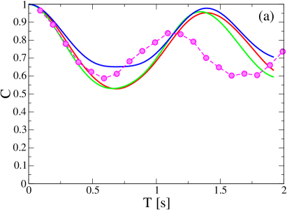
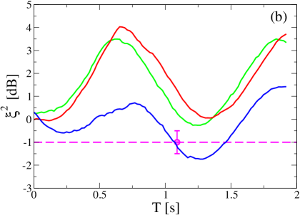
Figure 7: Contrast (a) and Spin squeezing (b) as a function of time. Solid lines: Wigner simulations, including spatial dynamics, quantum spin dynamics and particle losses, for three different choices of the scattering lengths. Symbols: experiment (for (b), the experimental squeezing is measured at the time corresponding to the first contrast revival). The initial atom number is $N=10^{4}$. Trap frequencies $\omega_{x,y,z}=2\pi\times(2.9,92,74)$Hz. Lifetime $\tau=5$s. Two-body loss rate constants $\gamma_{22}=8.1\times 10^{-14}$cm${}^{3}/$s and $\gamma_{12}=1.51\times 10^{-14}$cm${}^{3}/$s. Scattering lengths in Bohr radii units: $a_{11}=100.4$ for the three curves. Red curve $a_{22}=95.44$ [30], $a_{12}=98.00$ [30]. Green curve $a_{22}=95.00$ [18], $a_{12}=97.66$ [18]. Blue curve $a_{22}=95.68$ [35], $a_{12}=97.66$ [18]. We used 800 realizations for the Wigner simulation. The statistical uncertainty is around $10\%$ for the spin squeezing, corresponding to 0.4dB on the figure. The spatial grid had $128\times 8\times 8$ points in the three directions and the initial temperature is zero. At the squeezing time in the simulation $T\simeq 1.37$s, approximately $N_{\text{f}}\simeq 6000$ atoms are left in the trap, in a proportion $N_{1f}/N_{2f}\simeq 5/3$ for the two states.

In Fig. 7 we show the results of the projected Wigner simulation for an initial atom number $N_{\text{i}}=10^{4}$ and three different choices of the scattering lengths $a_{12}$ and $a_{22}$ chosen among published values that differ by $0.7\%$ at most. Fig. 7(a) shows the contrast and Fig. 7(b) shows the squeezing as a function of time. The experimental data for similar parameters is shown as symbols for comparison. Given that the demixing dynamics which induces the squeezing is driven by the small differences between the scattering lengths, it is not surprising that, in the absence of an external state-dependent potential imposing the spatial separation [21, 4], the squeezing result is very sensitive to the precise values of the scattering lengths. To estimate the effective nonlinearity for the different choices of the scattering lengths, we calculated the parameter $\chi$ of the one-axis twisting Hamiltonian at the stationary state in our geometry. We obtain $\chi=7.5\times 10^{-5}$s^-1 with the scattering length values from [30] (red curve), $\chi=7.3\times 10^{-5}$s^-1 with the values from [18] (green curve), and $\chi=24.6\times 10^{-5}\,\mbox{s}^{-1}$ for the combination [18]-[35] (blue curve).

Comparing simulations and experiment, the contrast oscillations in the experiment have a smaller amplitude and shorter period than in the simulations (Fig. 7(a)), as was already observed with the GPE simulations. For the squeezing factor, the simulations do not allow a quantitative comparison to experiment due to their strong dependence on the scattering lengths. As shown in Fig. 7(b), depending on the choice of the scattering length values, and despite their relatively high accuracy (compared to the values available for other elements), the prediction at the revival time varies between no squeezing at all and about -1.8 dB.

We conclude that spontaneous squeezing in our geometry is compatible with the results of our simulations although we cannot reproduce all the features of the experimental data. If a quantitative agreement for the contrast dynamics can be attained, it would be interesting to use the extreme sensitivity to the scattering lengths to infer very precise values for them from the experiment, similar to [30].

7 Conclusion and outlook

Our results show that nonclassical spin dynamics occur spontaneously in a two-component BEC, and can produce spin squeezing in BECs with sizeable atom numbers. This supports the notion of squeezing as a naturally occuring form of entanglement. In order to use this squeezing as a resource for quantum metrology in particular, a higher level of squeezing is desirable. Our results suggest several possible routes. The first is to accelerate the component separation, so that squeezing would be produced on a faster timescale, before particle losses become dominant. To do this, it would suffice to induce a small asymmetry between the trapping potential of the two states at the beginning of the sequence, in order to help the dynamics to start. It has indeed been shown that this greatly enhances and accelerates the spatial separation [36]. In our case, this asymmetry could come from the combination of the quadratic Zeeman effect with gravity. This leads to a displacement of the center of the trapping potentials for the two clock states that depends on the difference between the field at the bottom of the trap and the magic field [37]. Therefore, by scanning the magnetic field at the trap bottom, one could displace the position of the two states and study its influence on the spatial dynamics. In the same spirit, it would be interesting to study whether the component separation can be improved by modifying the aspect ratio of the trap, perhaps dynamically.

Another path would be to act on the asymmetric two-body losses themselves to reduce their rate. A possible approach could be to use microwave dressing during the interrogation time to shift the $\left|2,2\right\rangle$ state upward and induce an energy difference between the transitions $\left|2,1\right\rangle\rightarrow\left|2,2\right\rangle$ and $\left|2,1\right\rangle\rightarrow\left|2,0\right\rangle$, thereby reducing the two-body collision rate in state $\left|2,1\right\rangle$. This could be accomplished using a one-photon dressing with a $\sigma$-polarized microwave field. Of course, one would need to check that this additional coupling does not introduce too much noise on the clock transition. Observing a reduction of these losses would also be an interesting subject in itself.

Appendix A Imaging and Calibration

Detection

For accurate, low-noise atom number measurement, we use saturated absorption imaging [31] along the slow $x$ axis, combined with spatially separated detection of both clock states in the same image, and employ back-illuminated deep depletion CCD camera with $>90\%$ quantum efficiency (Andor iKon M 934-BRDD). After the sequence but still in trap, atoms in $\left|1\right\rangle$ are adiabatically transferred to the untrapped $\left|F=2,m_{F}=0\right\rangle$ state in 2 ms by a strong MW pulse while the atomic resonance is swept by ramping the magnetic bias field $B_{x}$. Adiabaticity is ensured by Blackman pulse shape for the MW power and a half-Blackman ramp for $B_{x}$ ($\pm 50$mG around the pseudo-magic field). During this pulse, atoms initially in state $\left|1\right\rangle$ start to fall under the action of gravity. 50 $\mu$s later, the trapping magnetic fields are turned off in order to release the remaining atoms, such that the two states can be spatially discriminated after 23 ms time of flight and imaged with a single 20 $\mu$s detection pulse. This way, frequency and power fluctuations of the probe laser are in common mode for the two states, reducing fluctuations in the detected population difference. Additionally, a numerical frame re-composition algorithm is used to reduce optical fringes [38]. The column density is then derived taking into account the high saturation correction [31]. With this imaging procedure, the background noise of our imaging system is about 33 atoms for each of the spin components (cf. Fig. 8 (a)).

Great care is taken to calibrate the detection system. The calibration method is similar to [4], and consists in comparing the variance of $S_{z}$ for an ensemble of $N$ uncorrelated atoms in a coherent superposition with the standard quantum limit that scales as $\frac{N}{4}$. To perform the calibration, $S_{z}$ is measured directly after a single resonant $\frac{\pi}{2}$-pulse, and the measured variance is plotted as a function of the total detected atom number $N_{\text{f}}$. The data is fitted with $\sigma^{2}(S_{z})=\sigma_{det}^{2}+\sigma_{qpn}^{2}\overline{N}+\sigma_{tech}^{2}\overline{N}^{2}$, where $\sigma_{det}$ is the detection noise, $\sigma_{qpn}$ represents the quantum projection noise and $\sigma_{tech}$ accounts for the possible preparation noise. As shown in Fig. 8 (a), the atomic noise exhibits the expected linear behavior with a slope of $\sigma_{qpn}^{2}=0.248\pm 0.03$ and a neglegible quadratic component, $\sigma_{tech}^{2}=(1\pm 3)\times 10^{-6}$, confirming that our detection is projection noise limited.

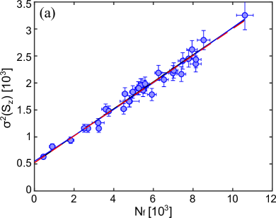
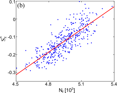
Figure 8: (a) Validation of the detection calibration. The variance of $S_{z}$ measured right after a single resonant $\frac{\pi}{2}$-pulse is plotted as a function of the detected atom number. Both the parabolic (blue line) and linear (red dashed line) fits give a linear part compatible with the standard quantum limit and a detection noise $\sigma_{det}\approx 33$ atoms. (b) Atom number correlation for $\alpha=90^{\circ}$.

Data analysis

In order to link the measured atom numbers to the squeezing factor and the spin noise distribution, the following data analysis is performed for each tomography angle $\alpha$. The notation $\overline{X}$ corresponds to the average of the fluctuating quantity X, and the error bars correspond to one standard deviation.

• Shots whose total atom numbers $N_{\text{f}}=N_{1}+N_{2}$ differ from their mean $\overline{N}$ by more than 3 standard deviations are discarded. These outliers can be due to problems during the image acquisition or the laser locks, and in practice this concerns about 1$\%$ of the data.

• The normalized population difference $S_{z}^{n}=\frac{N_{2}-N_{1}}{2N_{\text{f}}}$ and the angle between the collective spin and the equator of the Bloch sphere $\theta_{c}=\text{asin}(\frac{S_{z}^{n}}{C/2})$ are derived, where $C$ is the contrast of the Ramsey interferometer, which has been measured separately. The population difference is normalized in order to reduce its dependency to shot-to-shot total atom number fluctuations.

• A correlation between population difference and total atom number exists because of the atom number dependency of the atomic frequency ($1.5\times 10^{-4}$ Hz per atom) via the collisional shift [19], and can be estimated by fitting the distribution $S_{z}^{n}$ vs $N_{\text{f}}$ (cf. Fig. 8 (b)). Since we can measure this correlation for each shot, we can legitimately correct the data accordingly. Namely,

  $$S_{z,corr}^{n}(i)=S_{z}^{n}(i)-s_{p}\times(N_{\text{f}}(i)-\overline{N_{\text{f}}}),$$ (9)

  where $s_{p}=\frac{dS_{z}^{n}}{dN_{\text{f}}}$ is the slope measured on Fig. 8 (b) and $i$ represents one of the 300 shots at a given rotation angle. This slope, and thus the correction, depends on the analysis pulse duration and happens to vanish around $\alpha=2.5^{\circ}$; it therefore does no affect the squeezing factor.

• The variance of the normalized population difference times the mean atom number $\overline{N_{\text{f}}}\sigma^{2}(S_{z,corr}^{n})$ is derived. At this point, we also check that the Allan variance of $S_{z,corr}^{n}$ integrates as white frequency noise in order to be sure that there is no drift that could worsen the results.

• The detection noise estimated in Fig. 8 (a) is removed from the data:

  $$\Delta S_{z}^{2}=\overline{N_{\text{f}}}^{2}\sigma^{2}(S_{z,corr}^{n})-\sigma_{det}^{2}(S_{z})$$ (10)

• Finally, the fact that the collective spin ends up below the equator of the Bloch sphere leads to an underestimation of the spin noise by a factor $\text{cos}(\overline{\theta_{c}})^{2}$ which has to be taken into account as explained in sec. 3. $\Delta S_{z}^{2}$ is then normalized by the quantum projection noise $N_{\text{f}}/4$, leading to the final number squeezing and squeezing factor [8]

  $$\mathcal{V}^{2}=\frac{4\Delta S_{z}^{2}}{\overline{N_{\text{f}}}\text{cos}(\overline{\theta_{c}})^{2}}\text{ and }\xi^{2}=\frac{4\Delta S_{z}^{2}}{\overline{N_{\text{f}}}C^{2}\text{cos}(\overline{\theta_{c}})^{2}}.$$ (11)

Analysis pulse calibration

In order to perform the state tomography, one could in principle apply the correction pulse discussed in sec. 3 prior to the analysis pulse, which would simply need to be phase shifted with respect to the preparation pulse. However, because of microwave inhomogeneity and position fluctuation of the trapped BEC, this correction pulse would introduce additional noise in the spin tomography sequence. The idea is then to keep the Bloch vector below the equator of the Bloch sphere, and align the Rabi vector of the analysis pulse with the Bloch vector to rotate the noise distribution about its center. The z-component of the Rabi vector is given by the detuning between the considered pulse $\nu_{lo}$ and the instantaneous atomic frequency $\nu_{at}$ at the time at which the pulse is applied. The azimuthal angle is controlled via the phase shift with respect to the first pulse. First one needs to measure $\nu_{at}$, which is the frequency for which the resulting transition probability does not depend on the local oscillator phase-shift when the analysis pulse is a $\pi-$pulse. The detuning $\nu_{lo}-\nu_{at}$ is then simply given by $\pm\frac{\Omega_{R}}{2\pi}\text{tan}(\theta_{c})$. The $"\pm"$ sign gives the direction of rotation performed during the tomography. Finally, the phase-shift that aligns the two vectors is the one that makes the resulting transition probability independent of the analysis pulse duration for the previously derived frequency.

Appendix B Test of the projected Wigner method

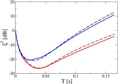
Figure 9: Test of the projected Wigner method against an exact solution of the two-mode model with and without losses, in a situation in which the spatial dynamics of the condensate wave functions is not excited. Spin squeezing as a function of time without losses (lower curves) and with asymmetric two-body losses (upper curves). Comparison between the projected Wigner simulation (solid lines) and a two-mode Monte Carlo simulation (dashed lines) with 1600 realizations. The initial atom number is $N=10^{4}$. Trap frequencies $\omega_{x,y,z}=2\pi\times(2.9,92,74)$Hz. Lifetime $\tau=5$s. Two-body loss rate constants $\gamma_{22}=8.1\times 10^{-14}$cm${}^{3}/$s and $\gamma_{12}=1.51\times 10^{-14}$cm${}^{3}/$s. Scattering lengths $a_{11}(0^{-})=100.4a_{0}$, $a_{11}(0^{+})=a_{22}(0^{+})=2a_{11}(0^{-})$ and $a_{12}=0$. We used 400 realizations for the Wigner simulation. At the end of the simulation, $\omega_{x}T=3$, approximately $N_{\text{f}}\simeq 9400$ atoms are left in the trap, in a proportion $N_{1f}/N_{2f}\simeq 0.515/0.485$ for the two states. For the two-mode model we used $\chi=0.064$s^-1, calculated at steady state after the pulse.

To test the projected Wigner method, we compared its results with an exact solution of the two-mode model with losses [32], in a situation in which the spatial dynamics of the condensate wave functions is not excited. To this end we choose $g_{ab}=0$, $g_{aa}=g_{bb}=g$, and the value of $g$ was doubled after the mixing pulse to keep the mean field constant. For the two-mode model we calculated the corresponding parameter $\chi$ of the one-axis twisting Hamiltonian and solved the corresponding master equation using the Monte Carlo wave function method with a large number of realizations. As $g_{ab}=0$, the nonlinearity is large and the squeezing generation is fast with respect to the losses, so that the squeezing factor gets very small which makes a good test for the projected Wigner method. As shown in Fig. 9, we find a good agreement between the two methods.

References

References

- [1] Kawaguchi Y and Ueda M 2012 Physics Reports 520 253
- [2] Esteve J, Gross C, Weller A, Giovanazzi S and Oberthaler M K 2008 Nature 455 1216
- [3] Gross C, Zibold T, Nicklas E, Estève J and Oberthaler M K 2010 Nature 464 1165
- [4] Riedel M F, Böhi P, Li Y, Hänsch T W, Sinatra A and Treutlein P 2010 Nature 464 1170
- [5] Lücke B, Scherer M, Kruse J, Pezzé L, Deuretzbacher F, Hyllus P, Topic O, Peise J, Ertmer W, Arlt J, Santos L, Smerzi A and Klempt C 2011 Science 334 773
- [6] Schmied R, Bancal J D, Allard B, Fadel M, Scarani V, Treutlein P and Sangouard N 2016 Science 352 441
- [7] Kitagawa M and Ueda M 1993 Phys. Rev. A 47 5138
- [8] Wineland D J, Bollinger J J, Itano W M and Heinzen D J 1994 Phys. Rev. A 50 67
- [9] Gross C 2012 J. Phys. B: At. Mol. Opt. Phys. 45 103001
- [10] Abend S, Gebbe M, Gersemann M, Ahlers H, Müntinga H, Giese E, Gaaloul N, Schubert C, Lämmerzahl C, Ertmer W, Schleich W P and Rasel E M 2016 Phys. Rev. Lett. 117 203003
- [11] Hardman K S, Everitt P J, McDonald G D, Manju P, Wigley P B, Sooriyabandara M A, Kuhn C C N, Debs J E, Close J D and Robins N P 2016 Phys. Rev. Lett. 117 138501
- [12] Sørensen A, Duan L M, Cirac J I and Zoller P 2001 Nature 409 63
- [13] Haine S A, Lau J, Anderson R P and Johnsson M T 2014 Phys. Rev. A 90 023613
- [14] Pezzè L, Smerzi A, Oberthaler M, Schmied R and Treutlein P 2017 arxiv:1609.01609
- [15] Li Y, Treutlein P, Reichel J and Sinatra A 2009 Eur. Phys. J. B 68 365
- [16] Sinatra A, Dornstetter J C and Castin Y 2012 Front. Phys. 7 86
- [17] Maussang K, Marti G E, Schneider T, Treutlein P, Li Y, Sinatra A, Long R, Estève J and Reichel J 2010 Phys. Rev. Lett. 105 080403
- [18] Mertes K, Merrill J, Carretero-González R, Frantzeskakis D, Kevrekidis P and Hall D 2007 Phys. Rev. Lett. 99 190402
- [19] Harber D M, Lewandowski H J, McGuirk J M and Cornell E A 2002 Phys. Rev. A 66 053616
- [20] Szmuk R, Dugrain V, Maineult W, Reichel J and Rosenbusch P 2015 Phys. Rev. A 92 012106
- [21] Hall D S, Matthews M R, Ensher J R, Wieman C E and Cornell E A 1998 Phys. Rev. Lett. 81 1539
- [22] Egorov M, Anderson R P, Ivannikov V, Opanchuk B, Drummond P, Hall B V and Sidorov A I 2011 Phys. Rev. A 84 021605
- [23] Nicklas E, Muessel W, Strobel H, Kevrekidis P and Oberthaler M 2015 Phys. Rev. A 92 053614
- [24] Lacroute C, Reinhard F, Ramirez-Martinez F, Deutsch C, Schneider T, Reichel J and Rosenbusch P 2010 IEEE Transactions on Ultrasonics, Ferroelectrics and Frequency Control 57 106
- [25] Deutsch C, Ramirez-Martinez F, Lacroûte C, Reinhard F, Schneider T, Fuchs J N, Piéchon F, Laloë F, Reichel J and Rosenbusch P 2010 Phys. Rev. Lett. 105 020401
- [26] Treutlein P, Hommelhoff P, Steinmetz T, Hänsch T W and Reichel J 2004 Phys. Rev. Lett. 92 203005
- [27] Ramirez-Martinez F, Lours M, Rosenbusch P, Reinhard F and Reichel J 2010 IEEE Transactions on Ultrasonics, Ferroelectrics and Frequency Control 57 88
- [28] Papp S B, Pino J M and Wieman C E 2008 Phys. Rev. Lett. 101 040402
- [29] Tojo S, Taguchi Y, Masuyama Y, Hayashi T, Saito H and Hirano T 2010 Phys. Rev. A 82 033609
- [30] Egorov M, Opanchuk B, Drummond P, Hall B, Hannaford P and Sidorov A 2013 Phys. Rev. A 87 053614
- [31] Reinaudi G, Lahaye T, Wang Z and Guéry-Odelin D 2007 Opt. Lett. 32 3143
- [32] Li Y, Castin Y and Sinatra A 2008 Phys. Rev. Lett. 100 210401
- [33] Opanchuk B, Egorov M, Hoffmann S, Sidorov A I and Drummond P D 2012 Europhys. Lett. 97 50003
- [34] Sinatra A, Lobo C and Castin Y 2002 J. Phys. B: At. Mol. Opt. Phys. 35 3599
- [35] Kokkelmans S J J M F 2013 private communication, cited in [30]
- [36] Ockeloen C F, Schmied R, Riedel M F and Treutlein P 2013 Phys. Rev. Lett. 111 143001
- [37] Rosenbusch P 2009 Applied Physics B: Lasers and Optics 95 227
- [38] Ockeloen C F, Tauschinsky A F, Spreeuw R J C and Whitlock S 2010 Phys. Rev. A 82 061606