Extending the Best Linear Approximation Framework to the Process Noise Case

Abstract

The Best Linear Approximation (BLA) framework has already proven to be a valuable tool to analyze nonlinear systems and to start the nonlinear modeling process. The existing BLA framework is limited to systems with additive (colored) noise at the output. Such a noise framework is a simplified representation of reality. Process noise can play an important role in many real-life applications.

This paper generalizes the Best Linear Approximation framework to account also for the process noise, both for the open-loop and the closed-loop setting, and shows that the most important properties of the existing BLA framework remain valid. The impact of the process noise contributions on the robust BLA estimation method is also analyzed.

1 Introduction

A linear approximate model of a nonlinear system often offers valuable insight into the linear (but also nonlinear) behavior of that system. The Best Linear Approximation (BLA) framework described in (Schoukens et al., 1998; Pintelon and Schoukens, 2002; Enqvist, 2005; Enqvist and Ljung, 2005; Schoukens et al., 2009; Pintelon and Schoukens, 2012a) offers such a well understood and valuable approximation framework for a wide class of practically important signals and systems (see in detail in Section 2). The BLA framework is often used to analyze how nonlinearly a system behaves (see for instance (Vaes et al., 2015) for mechanical systems and (Vlaar et al., 2017) for biomechanical systems), to guide the user to select a good nonlinear model structure (Schoukens et al., 2015), to obtain linear models in the presence of nonlinearities (Pintelon and Schoukens, 2012a), but also to start the estimation process of a nonlinear model (Paduart et al., 2010; Schoukens, 2017; Schoukens and Tiels, 2017). A recent overview of the BLA framework, and its use in practical applications (e.g. ground vibration testing, combustion engine, robotics and electronics), is provided in (Schoukens et al., 2016).

The BLA framework was initially defined for systems operating in open loop and with additive (colored) noise present at the output only. The extension towards the closed-loop setting has been made in (Pintelon and Schoukens, 2012b, 2013). The extension of the BLA framework to include process noise is the subject of this paper.

Considering additive (colored) noise at the output only is a simplified representation of reality. This simplification can lead to biased nonlinear model estimates when other noise sources are present, located at other positions inside the system, e.g. process noise passing through a nonlinear subsystem (Hagenblad et al., 2008). A more realistic noise framework can be obtained by introducing multiple noise sources, or by placing the noise source at another location in the model structure. It is important to offer the user a theoretical framework with which (s)he can analyze the influence of process noise on the system, and whether or not it is important to include process noise in the nonlinear modeling step. An extended BLA framework could offer this theoretical insight. An initial step towards a generalized BLA analysis is made in (Giordano and Sjöberg, 2016) where the BLA of a Wiener-Hammerstein system is analyzed in the presence of process noise.

This paper introduces first the classical open-loop BLA framework with additive noise at the system output only (Section 2). The extension towards systems with process noise is presented in Section 3. It is shown in Section 4 that this extension is also valid for systems operating in closed loop. The impact of the process noise contributions on the robust BLA estimation method is analyzed in Section 5. Finally, the proposed process noise BLA framework is illustrated in Section 6. A discrete-time setting is used throughout the paper. However, all derivations and proofs can easily be generalized to the continuous-time setting.

2 Best Linear Approximation: Additive Noise at the System Output

Figure 1: A dynamic nonlinear system with zero-mean (colored) additive noise $n_{y}(t)$ at the output only. The input excitation $u(t)$ belongs to the signal class $\mathbb{U}$.

2.1 Signal Class

This paper assumes the input signal $u(t)$ (see Figure 1) to belong to a generalization of the Gaussian signal class: the Riemann equivalence class of asymptotically normally distributed excitation signals (Schoukens et al., 2009; Pintelon and Schoukens, 2012a). Note that the BLA can also be defined for other signal classes. This choice has been made here to follow the framework defined in (Pintelon and Schoukens, 2012a), and to use the same class of systems. However, many of the properties that are derived in this paper are not limited to the chosen input signal class. The impact of the input signal class is studied in (Wong et al., 2012).

Definition 1.

Riemann equivalence class of asymptotically normally distributed excitation signals $\mathbb{U}$. Consider a signal $u(t)$ with a power spectrum $S_{UU}(j\omega)$. $S_{UU}(j\omega)$ is piecewise continuous, with a finite number of discontinuities. A random signal $u(t)$ belongs to the Riemann equivalence class if it obeys any of the following statements:

1. $u(t)$ is a Gaussian process with power spectrum $S_{UU}(j\omega)$.

2. $u(t)$ is a random multisine or random phase multisine (Pintelon and Schoukens, 2012a) such that:

$$\frac{1}{N}\sum_{k=k_{1}}^{k_{2}}E\left\{\left|U\left(j\omega_{k}\right)\right|^{2}\right\} =\frac{1}{2\pi}\int_{\omega_{k_{1}}}^{\omega_{k_{2}}}S_{UU}\left(j\nu\right)d\nu+O\left(\frac{1}{N}\right),$$

with $\omega_{k}=k\frac{2\pi f_{s}}{N}$, $k\in\mathbb{N}$, $0\leq\omega_{k_{1}}<\omega_{k_{2}}<\pi f_{s}$, $f_{s}$ is the sampling frequency.

A random phase multisine $u(t)$ is a periodic signal with period length $\frac{N}{f_{s}}$, where $N$ is the number of samples in one period, defined in (Pintelon and Schoukens, 2012a) as:

$$u(t) =\frac{1}{\sqrt{N}}\sum_{k=0}^{N/2-1}2U_{k}\cos(2\pi k\frac{t}{N}+\varphi_{k}).$$ (1)

The phases $\varphi_{k}$ are random variables that are independent over the frequency and are a realization of a random process on $[0,2\pi[$, such that $E\{e^{j\varphi_{k}}\}=0$. For instance, the random phases can be uniformly distributed between $[0,2\pi[$. The (real) amplitude $U_{k}$ is set in a deterministic way by the user. $U_{k}$ is uniformly bounded by $M_{U}$ ($0\leq U_{k}\leq M_{U}<\infty$).

Note that the Riemann equivalence class of asymptotically normally distributed excitation signals can, in most cases, easily be tuned to fit the application at hand, without much additional processing or hardware. The random phase multisine signals are periodic excitation signals, offering the opportunity of leakage-free measurements with a full control on the amplitude spectrum.

2.2 System Class and Noise Framework

It is assumed that the nonlinear system output can be represented arbitrarily well in the least-squares sense by a fading memory Volterra kernel representation (Schetzen, 1980; Boyd and Chua, 1985). This system class contains, for instance, systems with a hard saturation nonlinearity, but does not contain bifurcating and chaotic systems. The generality of this system class is discussed in detail by (Boyd and Chua, 1985).

The Volterra model output consists of the sum of the outputs of the kernels of different degree. The output of a Volterra kernel of degree $\alpha$ is given by in the time domain by:

$$y_{\alpha}(t) =V_{\alpha}(u(t)),$$ (2)

$$=\sum_{k_{1},\ldots,k_{\alpha}=0}^{N_{k}}h_{\alpha}(k_{1},\ldots,k_{\alpha})u(t-k_{1})\ldots u(t-k_{\alpha}),$$

which results in the following frequency domain representation:

$$Y_{\alpha}(j\omega_{k}) =\frac{1}{N^{\frac{\alpha-1}{2}}}\sum_{k_{1},k_{2},\ldots,k_{\alpha-1}=-N/2+1}^{N/2-1}H^{\alpha}_{L_{k},k_{1},k_{2},\ldots,k_{\alpha-1}}$$

$$\quad\quad\quad U(j\omega_{L_{k}})U(j\omega_{k_{1}})\ldots U(j\omega_{k_{\alpha-1}}),$$ (3)

where $L_{k}=k-k_{1}-k_{2}-\ldots-k_{\alpha-1}$. $H^{\alpha}_{L_{k},k_{1},k_{2},\ldots,k_{\alpha-1}}$ is a symmetrized frequency domain representation of the Volterra kernel $h_{\alpha}$ of degree $\alpha$ (Schetzen, 1980; Pintelon and Schoukens, 2012a). $Y_{\alpha}(j\omega_{k})$ is obtained as the Discrete Fourier Transform (DFT) of $y_{\alpha}(t)$:

$$Y_{\alpha}(j\omega_{k})=\frac{1}{\sqrt{N}}\sum_{t=0}^{N-1}y_{\alpha}(t)e^{-j2\pi tk/N},$$ (4)

$$y_{\alpha}(t)=\frac{1}{\sqrt{N}}\sum_{k=0}^{N-1}Y_{\alpha}(j\omega_{k})e^{j2\pi tk/N}.$$ (5)

Definition 2.

$\mathbb{S}$ is the class of nonlinear systems such that, when excited by a random phase multisine:

$$\exists\;C_{1}<\infty,\text{s.t.}\;\sum_{\alpha=1}^{\infty}M_{G^{\alpha}}M^{\alpha}_{U}\leq C_{1},$$ (6)

with $M_{G^{\alpha}}=\textit{max}\left|H^{\alpha}_{L_{k},k_{1},k_{2},\ldots,k_{\alpha-1}}\right|$, where the maximum is taken over the indices $L_{k},k_{1},k_{2},\ldots,k_{\alpha-1}$.

Definition 2 postulates the existence of a uniformly bounded fading memory Volterra series whose output converges in mean square sense to the output of the nonlinear system belonging to the system class $\mathbb{S}$ (see (Pintelon and Schoukens, 2012a) for more detail) when the degree $\alpha$ grows to infinity.

Assumption 1.

Output noise framework: An additive, colored zero-mean noise source $n_{y}(t)$ with a finite variance $\sigma_{n_{y}}^{2}$ is present at the output of the system (see Figure 1):

$$y(t)=y_{0}(t)+n_{y}(t).$$ (7)

This noise $n_{y}(t)$ is assumed to be independent of the known input $u(t)$. $y(t)$ is the actual measured output signal and a subscript $0$ denotes the exact (noise-free) value.

2.3 Definition of the Best Linear Approximation

The BLA model of a nonlinear system belonging to system class $\mathbb{S}$ with zero-mean (colored) additive noise at the system output only (see Figure 1) is a linear time-invariant (LTI) approximation of the behavior of that system. The BLA is defined in (Schoukens et al., 1998; Pintelon and Schoukens, 2002; Schoukens et al., 2009; Pintelon and Schoukens, 2012a) as:

$$G_{bla}(q) =\underset{G(q)}{\operatorname*{arg\;min}}\>E_{u,n_{y}}\left\{\left|\tilde{y}(t)-G(q)\tilde{u}(t)\right|^{2}\right\},$$ (8)

$$\tilde{u}(t) =u(t)-E_{u}\left\{u(t)\right\},$$ (9)

$$\tilde{y}(t) =y(t)-E_{u,n_{y}}\left\{y(t)\right\},$$ (10)

where $E_{u,n_{y}}\left\{.\right\}$ denotes the expected value operator taken w.r.t. the random variations due to the input $u(t)$ and the output noise $n_{y}(t)$ and $G(q)$ belongs to the set of all possible LTI systems. This definition of the BLA is equivalent to the definition of the linear time-invariant second-order equivalent model defined in (Ljung, 2001; Enqvist, 2005; Enqvist and Ljung, 2005) when the stability and causality restrictions imposed there are omitted.

It is shown that the BLA is given by (Enqvist, 2005; Enqvist and Ljung, 2005; Pintelon and Schoukens, 2012a):

$$G_{bla}(j\omega)=\frac{S_{YU}(j\omega)}{S_{UU}(j\omega)},$$ (11)

where $S_{YU}(j\omega)$ is the cross-power spectrum of $u(t)$ and $y(t)$ and $S_{UU}(j\omega)$ is the autopower spectrum of $u(t)$. Hence, the existence of $G_{bla}(j\omega)$ is guaranteed if $S_{UU}(j\omega)$ and $S_{YU}(j\omega)$ exist, and $S_{UU}(j\omega)\neq 0$. The existence of $S_{YU}(j\omega)$ is guaranteed by the chosen signal (Definition 1) and system class (Definition 2) (Pintelon and Schoukens, 2012a; Schetzen, 1980). The BLA is not defined at the frequencies where $S_{UU}(j\omega)=0$ (Enqvist, 2005; Pintelon and Schoukens, 2012a). A (possible infinite order, noncausal) transfer function or impulse response representation $G_{bla}(q)$ can be obtained by fitting $G_{bla}(j\omega)$ at the excited frequencies.

Figure 2: The BLA of a nonlinear system for a given class of excitation signals $\mathbb{U}$ consists of the resulting LTI model $G_{bla}(q)$, the stochastic nonlinear contribution $y_{s}(t)$, and the noise distortion $y_{n}(t)$.

Three constituents of the BLA framework can be defined (see Figure 2): the BLA $G_{bla}(q)$ itself, the stochastic nonlinear contribution $y_{s}(t)$ and the noise contribution $y_{n}(t)$. The output residuals $y_{t}(t)$ represent the total distortion that is present at the output of the system. The total distortion can be split in two contributions based on their nature as is depicted in Figure 2. The stochastic nonlinear contribution $y_{s}(t)$ represents the unmodeled nonlinear contributions, while the noise contribution ${y}_{n}(t)$ is the additive noise that is present at the system output:

$$y_{t}(t) =\tilde{y}(t)-G_{bla}(q)\tilde{u}(t)=y_{s}(t)+y_{n}(t),$$ (12)

$$y_{s}(t) =\tilde{y}_{0}(t)-G_{bla}(q)\tilde{u}(t),$$ (13)

$$y_{n}(t) =\tilde{y}(t)-\tilde{y}_{0}(t)=n_{y}(t),$$ (14)

where $\tilde{y}_{0}(t)=E_{n_{y}}\{\tilde{y}(t)\}$ is the unknown zero-mean noiseless output. The nonlinear distortion $y_{s}(t)$ is linearly uncorrelated with the input $\tilde{u}(t)$ ($E_{u}\{y_{s}(t)\tilde{u}(\tau)\}=0\>\forall\>t,\tau$). The nonlinear distortion $y_{s}(t)$ is not independent of the input $\tilde{u}(t)$ however (Pintelon and Schoukens, 2012a). The noise distortion $y_{n}(t)$ on the contrary is both uncorrelated with the input and independent of the input $\tilde{u}(t)$. All three signals $y_{bla}(t)$, $y_{s}(t)$, $y_{n}(t)$ are zero-mean.

3 Best Linear Approximation: Process Noise Extension

3.1 Considered System Class and Noise Framework

The considered excitation signal class and the output noise assumptions are unchanged with respect to Section 2. The considered system class is extended here to include process noise, and the necessary assumptions on the process noise are formulated.

Figure 3: A dynamic nonlinear system with zero-mean (colored) process noise $n_{x}(t)$ and zero-mean (colored) additive output noise $n_{y}(t)$. The input excitation $u(t)$ belongs to the signal class $\mathbb{U}$.

It is assumed in Section 2.2 that the underlying nonlinear system is a Volterra system. Here we extend the standard single-input single-output Volterra kernel representation to a dual-input single-output representation where one of the inputs is excited by the process noise (see Figure 3). The modeling of the process noise as the second input to the Volterra system describing the measured nonlinear system opens considerable opportunities for a unified treatment of many process noise configurations. The output of a dual-input m,n-th order Volterra kernel with process noise is given by:

$$y_{m,n}(t) =V_{m,n}(u(t),n_{x}(t)),$$ (15)

$$=\sum_{k_{1},\ldots,k_{m}=0}^{N_{k}}\sum_{j_{1},\ldots,j_{n}=0}^{N_{j}}h_{m,n}(k_{1},\ldots,k_{m},j_{1},\ldots,j_{n})$$

$$\>\>u(t-k_{1})\ldots u(t-k_{m})n_{x}(t-j_{1})\ldots n_{x}(t-j_{n}),$$

where $N_{k}$ and $N_{j}$ are the numbers of taps considered for the input $u$ and the process noise $n_{x}$ respectively.

Assumption 2.

Process noise framework: A colored zero-mean noise source $n_{x}(t)$ is present as one of the inputs of the dual-input single-output Volterra representation of the nonlinear system.

$$y_{0}(t)=\sum_{m=0}^{\infty}\sum_{n=0}^{\infty}V_{m,n}(u(t),n_{x}(t))$$ (16)

The noise $n_{x}(t)$ is assumed to be independent of the known input $u(t)$ and the output noise $n_{y}(t)$, its $n$-th order moments are finite $\forall\>n\in\mathbb{N}$.

Theorem 1.

If $y_{m,n}(t)=V_{m,n}(u(t),n_{x}(t))$, then $\bar{\bar{y}}_{m,n}(t)=\bar{\bar{V}}_{m,n}(u(t))$, where

$$\bar{\bar{y}}_{m,n}(t) =E_{n_{x}}\{y_{m,n}(t)\}.$$ (17)

$$\bar{\bar{V}}_{m,n}(u(t)) =\sum_{k_{1},\ldots,k_{m}=0}^{N_{k}}\bar{\bar{h}}_{m,n}(k_{1},\ldots,k_{m})$$ (18)

$$\>\>u(t-k_{1})\ldots u(t-k_{m}),$$

$$\bar{\bar{h}}_{m,n}(k_{1},\ldots,k_{m}) =\sum_{j_{1},\ldots,j_{n}=0}^{N_{j}}h_{m,n}(k_{1},\ldots,k_{m},j_{1},\ldots,j_{n})$$

$$\>\>E_{n_{x}}\{n_{x}(t-j_{1})\ldots n_{x}(t-j_{n})\}$$ (19)

Proof 3.1.

The signal $\bar{\bar{y}}_{m,n}(t)$ is obtained by taking the expectation of (15) w.r.t. the process noise $n_{x}$:

$$\bar{\bar{y}}_{m,n}(t) =E_{n_{x}}\{y_{m,n}(t)\}$$ (20)

$$=\sum_{k_{1},\ldots,k_{m}=0}^{N_{k}}\sum_{j_{1},\ldots,j_{n}=0}^{N_{j}}h_{m,n}(k_{1},\ldots,k_{m},j_{1},\ldots,j_{n})$$

$$\>\>u(t-k_{1})\ldots u(t-k_{m})E_{n_{x}}\{n_{x}(t-j_{1})\ldots n_{x}(t-j_{n})\},$$

where the expectation $E_{n_{x}}\{n_{x}(t-j_{1})\ldots n_{x}(t-j_{n})\}$ depends on the $n$-th order moment of $n_{x}(t)$ and its decomposition into pairwise autocorrelations (Schetzen, 1980). This can be simplified using eq. (19):

$$\bar{\bar{y}}_{m,n}(t) =\sum_{k_{1},\ldots,k_{m}=0}^{N_{k}}\bar{\bar{h}}_{m,n}(k_{1},\ldots,k_{m})$$ (21)

$$\>\>u(t-k_{1})\ldots u(t-k_{m}),$$

$$=\bar{\bar{V}}_{m,n}(u(t)).$$ (22)

The sum in eq. (19) is finite since $h_{m,n}(k_{1},\ldots,k_{m},j_{1},\ldots,j_{n})$ is finite and it is assumed in Assumption 2 that the $n$-th order moments of the process noise $n_{x}(t)$ are finite.

This theorem shows that the relation between $u$ and $y$ is given by a SISO Volterra representation after taking the expectation of $y$ with respect to the random realization of the process noise.

Definition 3.

$\mathbb{S}_{p}$ is the class of nonlinear systems such that, when excited with a random phase multisine, the following inequality holds:

$$\exists\;C_{1}<\infty,\text{s.t.}\;\sum_{m=0}^{\infty}\sum_{n=0}^{\infty}M_{G^{m,n}}M^{m}_{U}\leq C_{1},$$ (23)

with $M_{G^{m,n}}=\textit{max}\left|\bar{\bar{H}}^{m,n}_{L_{k},k_{1},k_{2},\ldots,k_{m-1}}\right|$, where $\bar{\bar{H}}^{m,n}_{L_{k},k_{1},k_{2},\ldots,k_{m-1}}$ is the symmetrized frequency domain representation of $\bar{\bar{h}}_{m,n}(k_{1},\ldots,k_{m})$.

Definition 3 is the natural extension of the system class $\mathbb{S}$. Indeed when no process noise is present the system class $\mathbb{S}$ is obtained. The finite moment assumption on the process noise is also similar to the maximum amplitude restriction in Definition 2.

3.2 Generalized Definition of the Best Linear Approximation

The BLA framework in the presence of process noise is defined in this section. The framework consists of four model components: the BLA $G_{bla}(q)$ itself, the stochastic nonlinear distortion $y_{s}(t)$ due to the randomized input, the process noise contribution $y_{p}(t)$ due to the process noise, and the output noise contribution $y_{n}(t)$ as depicted in Figure 4. Note that the process noise contribution $y_{p}$ is a new constituent of the extended BLA framework due to the presence of process noise in the system.

Figure 4: The BLA of a nonlinear system for a given class of excitation signals $\mathbb{U}$ consists of the resulting LTI model $G_{bla}(q)$, the unmodeled nonlinear contribution $y_{s}(t)$, the process noise distortion $y_{p}(t)$ and the output noise distortion $y_{n}(t)$.

Two important design decisions are made in defining the extended BLA framework:

1. The BLA $G_{bla}(q)$ and the stochastic nonlinear distortion $y_{s}$ are defined such that they do not depend on the actual realization of $n_{x}$ and $n_{y}$.

2. The process noise contribution $y_{p}$ is defined such that it does not depend on the actual realization of the output noise $n_{y}$.

The BLA and the stochastic distortions $y_{s}$ are defined next as:

$$G_{bla}(q) =\underset{G(q)}{\operatorname*{arg\;min}}\>E_{u,n_{y},n_{x}}\left\{\left|\tilde{y}(t)-G(q)\tilde{u}(t)\right|^{2}\right\},$$ (24)

$$y_{s}(t) =\bar{\bar{y}}(t)-y_{bla}(t)=\bar{\bar{y}}(t)-G_{bla}(q)\tilde{u}(t),$$ (25)

where $G(q)$ belongs to the set of all possible LTI systems, and $\tilde{u}(t)$ is defined in eq. (9), $y_{bla}(t)=G_{bla}(q)\tilde{u}(t)$, $\bar{\bar{y}}(t)$ is defined as:

$$\bar{\bar{y}}(t) =E_{n_{x},n_{y}}\{\tilde{y}(t)\},$$ (26)

$\tilde{u}(t)$ and $\tilde{y}(t)$ are now defined as:

$$\tilde{u}(t) =u(t)-E_{u}\{u(t)\},$$ (27)

$$\tilde{y}(t) =y(t)-E_{u,n_{x},n_{y}}\{y(t)\}.$$ (28)

The process noise contribution $y_{p}$ is defined as:

$$y_{p}(t) =\bar{y}(t)-\bar{\bar{y}}(t),$$ (29)

$$=\tilde{y}_{0}(t)-G_{bla}(q)\tilde{u}(t)-y_{s}(t),$$ (30)

where $\bar{y}(t)$ is defined as:

$$\bar{y}(t) =E_{n_{y}}\{\tilde{y}(t)\},$$ (31)

$$=\tilde{y}_{0}(t).$$ (32)

The output noise contribution $y_{n}$, the final constituent of the BLA framework, remains to be defined:

$$y_{n}(t) =\tilde{y}(t)-\bar{y}(t),$$ (33)

$$=\tilde{y}(t)-\tilde{y}_{0}(t),$$ (34)

$$=\tilde{y}(t)-G_{bla}(q)\tilde{u}(t)-y_{s}(t)-y_{p}(t),$$ (35)

$$=n_{y}(t).$$ (36)

Note that, by definition, the noise contribution $y_{n}(t)=n_{y}(t)$. However, other choices for the definition of $y_{n}(t)$ may be made, resulting in different expressions of the noise contribution. This is highlighted in the last paragraph of Section 6.

To conclude we have that the system output $\tilde{y}(t)$, as shown in Figure 4, is given by:

$$\tilde{y}(t) =y_{bla}(t)+y_{s}(t)\quad \rightarrow \>E_{n_{x},n_{y}}\{\tilde{y}(t)\}$$ (37)

$$\>\>+y_{p}(t)\quad \rightarrow \>E_{n_{y}}\{\tilde{y}(t)\}-E_{n_{x},n_{y}}\{\tilde{y}(t)\}$$

$$\>\>+y_{n}(t)\quad \rightarrow \>\tilde{y}(t)-E_{n_{y}}\{\tilde{y}(t)\}$$

Section 5 presents how the BLA, and the variances of the signals $y_{p}(t)+y_{n}(t)$ and $y_{s}(t)+y_{p}(t)+y_{n}(t)$ can be estimated using the robust BLA estimation approach.

3.3 Properties of the BLA Model Components

This section shows that the stochastic nonlinear distortion $y_{s}(t)$ and the process noise contribution $y_{p}(t)$ are zero-mean, and linearly uncorrelated with - but not independent of - the input $\tilde{u}(t)$.

Theorem 2.

Properties of the stochastic nonlinear distortion and the process noise contribution.

• The stochastic nonlinear distortion $y_{s}(t)$ has zero-mean and is linearly uncorrelated with $\tilde{u}(t)$:

  $$E_{u}\{y_{s}(t)\} =0,$$ (38)

  $$E_{u}\{y_{s}(t)\tilde{u}(\tau)\} =0\quad\quad\forall\>t,\tau.$$ (39)

• The process noise contribution $y_{p}(t)$ has zero-mean and is linearly uncorrelated with $\tilde{u}(t)$:

  $$E_{n_{x}}\{y_{p}(t)\} =0,$$ (40)

  $$E_{n_{x}}\{y_{p}(t)\tilde{u}(\tau)\} =0\quad\quad\forall\>t,\tau.$$ (41)

• The sum of the process noise contribution $y_{p}(t)$ and the stochastic nonlinear contribution is uncorrelated with $\tilde{u}(t)$:

  $$E_{u,n_{x}}\{(y_{p}(t)+y_{s}(t))\tilde{u}(\tau)\}=0\quad\quad\forall\>t,\tau$$ (42)

Proof 3.2.

The expected value of the stochastic nonlinear distortion $y_{s}(t)$ with respect to the input signal realization is given by:

$$E_{u}\{y_{s}(t)\}=E_{u}\{\bar{\bar{y}}(t)\}-E_{u}\{G_{bla}(q)\tilde{u}(t)\}.$$ (43)

The second term is equal to zero since $\tilde{u}(t)$ is zero-mean by construction. The first term is given by:

$$E_{u}\{\bar{\bar{y}}(t)\} =E_{u,n_{x},n_{y}}\{\tilde{y}(t)\},$$ (44)

where $E_{u}\{\tilde{y}(t)\}$ is zero by construction. It hence follows directly from the definition of $y_{s}(t)$ that $E_{u}\{y_{s}(t)\}=0$.

The stochastic nonlinear distortion $y_{s}(t)$ is the residual of a linear least squares fit of a linear time-invariant model between $\bar{\bar{y}}(t)$ and $\tilde{u}(t)$ (see eq. (25)). Hence $y_{s}(t)$ is linearly uncorrelated with $\tilde{u}(t)$ by construction in the absence of model errors ($G(q)$ belongs to the set of all possible LTI systems).

The process noise contribution $y_{p}(t)$ is given by:

$$y_{p}(t) =\bar{y}(t)-\bar{\bar{y}}(t)$$

$$=E_{n_{y}}\{\tilde{y}(t)\}-E_{n_{x},n_{y}}\{\tilde{y}(t)\}.$$ (45)

The expected value $E_{n_{x}}\{y_{p}(t)\}$ taken over the process noise realization is thus given by:

$$E_{n_{x}}\{\bar{y}(t)\} =E_{n_{x},n_{y}}\{\tilde{y}(t)\}-E_{n_{x},n_{y}}\{\tilde{y}(t)\}=0.$$ (46)

The input $\tilde{u}$ does not depend on the process noise $n_{x}$ by construction and $E_{n_{x}}\{y_{p}(t)\}=0$ as is shown above. This results in:

$$E_{n_{x}}\{y_{p}(t)\tilde{u}(\tau)\} =E_{n_{x}}\{y_{p}(t)\}\tilde{u}(\tau)=0.$$ (47)

It follows directly from the proof above that $E_{u,n_{x}}\{(y_{p}(t)+y_{s}(t))\tilde{u}(\tau)\}=0\>\forall\>t,\tau$.

Many other properties of the BLA and its constituents can be proven based upon the assumption that the underlying nonlinear system is a Volterra system, and that the signal belongs to the Riemann equivalence class of asymptotically normally distributed excitation signals (Pintelon and Schoukens, 2012a). Section 3.1 showed that if the relationship between $\tilde{u}$, $n_{x}$ and $\tilde{y}$ is given by a Volterra system, then the relationship between $\tilde{u}$ and $\bar{\bar{y}}$ is also given by a Volterra system. As a consequence, the theoretical properties of $y_{s}$ and $G_{bla}$ proven for the basic case (see (Pintelon and Schoukens, 2012a) for an overview and a detailed analysis) still hold.

4 The Best Linear Approximation in Feedback

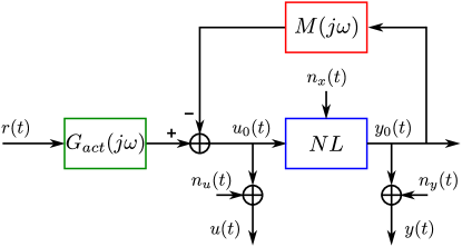
Figure 5: Setup for measuring the BLA of a nonlinear system with process noise operating in closed loop. The linear actuator and the feedback dynamics are represented by $G_{act}(j\omega)$ and $M(j\omega)$ respectively. $r(t)$ is the known reference signal, $u_{0}(t)$ and $y_{0}(t)$ are the noiseless input and output signal, $u(t)$ and $y(t)$ are the noisy input and output signal, and $n_{u}(t)$, $n_{y}(t)$ and $n_{x}(t)$ are the input measurement noise, output measurement noise and process noise respectively.

The classical open-loop BLA framework introduced in (Schoukens et al., 1998) has been extended to systems operating in closed loop (Pintelon and Schoukens, 2012b, 2013). The generalized BLA applicable to the process noise presented in this paper is complementary with the closed-loop theory and can be similarly extended to closed loop systems. (see Figure 5 for an overview of the setup).

The closed-loop BLA is defined using the indirect frequency response function measurement method for linear feedback systems (Wellstead, 1977, 1981), it is based upon the open-loop relations from the reference signal to the system input and the system output. Not only the the relation from the reference signal $r(t)$ to the output signal $y(t)$, but also the relation from $r(t)$ to the input signal $u(t)$ is assumed to belong to the system class $\mathbb{S}_{p}$.

Define:

$$\bar{\bar{y}}(t) =E_{n_{x},n_{y}}\{\tilde{y}(t)\},$$ (48)

$$\bar{\bar{u}}(t) =E_{n_{x},n_{u}}\{\tilde{u}(t)\}.$$ (49)

Where $\tilde{u}(t)$ and $\tilde{y}(t)$ are now defined as:

$$\tilde{u}(t) =u(t)-E_{r,n_{x},n_{u}}\{u(t)\},$$ (50)

$$\tilde{y}(t) =y(t)-E_{r,n_{x},n_{y}}\{y(t)\}.$$ (51)

The BLA of a nonlinear system with process noise operating in closed loop is now defined as:

$$G_{bla}(j\omega)=\frac{S_{\bar{\bar{Y}}R}(j\omega)}{S_{\bar{\bar{U}}R}(j\omega)},$$ (52)

where $S_{\bar{\bar{Y}}R}(j\omega)$ and $S_{\bar{\bar{U}}R}(j\omega)$ are the reference-output and reference-input cross-power spectra respectively.

The properties of the BLA of a system operating in feedback proven in (Pintelon and Schoukens, 2012b, 2013) can easily be brought over to the process noise case using the properties proven in this paper.

5 Estimating the BLA: the Robust Method

The BLA $G_{bla}(j\omega)$ can be estimated both parametrically or nonparametrically, an extensive review of the available BLA estimation techniques is provided by (Pintelon and Schoukens, 2012a; Schoukens et al., 2016). The presented methods remain valid in the process noise case. Some methods, such as the so-called robust method (Pintelon and Schoukens, 2012a; Schoukens et al., 2012, 2016), can also provide an estimate of the noise variance and the total variance. This section first recapitulates the robust BLA estimation method, the behavior of the robust method is analyzed in detail for the process noise case next.

5.1 The Robust Method: Algorithm

The robust BLA estimation approach makes use of multiple periods and multiple realizations of a random phase multisine. The estimated BLA $\hat{G}_{bla}(j\omega)$ in open loop and with a known input is obtained as follows (Pintelon and Schoukens, 2012a; Schoukens et al., 2012, 2016):

$$\hat{G}^{[m,p]}(j\omega) =\frac{Y^{[m,p]}(j\omega)}{U^{[m]}(j\omega)},$$ (53)

$$\hat{G}^{[m]}(j\omega) =\frac{1}{P}\sum_{p=1}^{P}\hat{G}^{[m,p]}(j\omega),$$ (54)

$$\hat{G}_{bla}(j\omega) =\frac{1}{M}\sum_{m=1}^{M}\hat{G}^{[m]}(j\omega),$$ (55)

where $Y^{[m,p]}(j\omega)$ is the DFT of the $p$-th period and $m$-th realization of the output signal $y(t)$, $U^{[m]}(j\omega)$ is the $m$-th realization of the input signal. Since $u(t)$ is noise free, it is equal over all periods. The noise variance $\hat{\sigma}_{bla,n}^{2}(j\omega)$ (the variance on $\hat{G}_{bla}(j\omega)$ due to $y_{n}(t)$ in the output noise setting) and total variance $\hat{\sigma}_{bla,t}^{2}(j\omega)$ (the variance on $\hat{G}_{bla}(j\omega)$ due to $y_{n}(t)+y_{s}(t)$ in the output noise setting) estimate are given by:

$$\hat{\sigma}_{bla,n}^{2}(j\omega) =\frac{1}{M^{2}P(P-1)}\sum_{m=1}^{M}\sum_{p=1}^{P}\left|\hat{G}^{[m]}(j\omega)-\hat{G}^{[m,p]}(j\omega)\right|^{2},$$ (56)

$$\hat{\sigma}_{bla,t}^{2}(j\omega) =\frac{1}{M(M-1)}\sum_{m=1}^{M}\left|\hat{G}_{bla}(j\omega)-\hat{G}^{[m]}(j\omega)\right|^{2}.$$ (57)

In order to quantify the variability of the mean BLA estimate (55), extra factors $M$ and $P$ have been introduced in the sample variances (56) and (57).

5.2 The Robust Method: Process Noise Analysis

The first step of the robust method takes the average of the output over the periods. Both the output noise contribution $y_{n}(t)$ and the process noise contribution $y_{p}(t)$ are aperiodic and zero-mean, while the stochastic nonlinear contribution is periodic. Hence, their contribution will be averaged out. In the second step, the average over the input realizations is taken. This step averages out the stochastic nonlinear contribution $y_{s}(t)$, but also the remaining contributions of the process noise and output noise $y_{p}(t)$ and $y_{n}(t)$. More formally we have that (see Figure 4):

$$Y^{[m,p]}(j\omega)=$$ (58)

$$Y^{[m]}_{bla}(j\omega)+Y^{[m]}_{s}(j\omega)+Y^{[m,p]}_{p}(j\omega)+Y^{[m,p]}_{n}(j\omega),$$

where $Y^{[m]}_{s}(j\omega)$, $Y^{[m,p]}_{p}(j\omega)$ and $Y^{[m,p]}_{n}(j\omega)$ are the DFT of the period $p$ and realization $m$ of the signals $y_{s}(t)$, $y_{p}(t)$ and $y_{n}(t)$ respectively. This results in the following expression for $\hat{G}^{[m,p]}(j\omega)$:

$$\hat{G}^{[m,p]}(j\omega)$$ (59)

$$=\frac{Y^{[m]}_{bla}(j\omega)}{U^{[m]}(j\omega)}+\frac{Y^{[m]}_{s}(j\omega)}{U^{[m]}(j\omega)}+\frac{Y^{[m,p]}_{p}(j\omega)+Y^{[m,p]}_{n}(j\omega)}{U^{[m]}(j\omega)},$$

$$=G_{bla}(j\omega)+\frac{Y^{[m]}_{s}(j\omega)}{U^{[m]}(j\omega)}+\frac{Y^{[m,p]}_{p}(j\omega)+Y^{[m,p]}_{n}(j\omega)}{U^{[m]}(j\omega)}.$$

A closer analysis, analogous to (Pintelon and Schoukens, 2012a), of the expected value of eq. (55), (56), (57) for the process noise case results in:

$$E\{\hat{G}_{bla}(j\omega)\} =G_{bla}(j\omega),$$ (60)

$$E\{\hat{\sigma}_{bla,n}^{2}(j\omega)\} =\frac{\sigma^{2}_{n}(j\omega)+\sigma^{2}_{p}(j\omega)}{MP|U(j\omega)|^{2}},$$ (61)

$$E\{\hat{\sigma}_{bla,t}^{2}(j\omega)\} =\frac{\sigma^{2}_{s}(j\omega)}{M|U(j\omega)|^{2}}+\frac{\sigma^{2}_{n}(j\omega)+\sigma^{2}_{p}(j\omega)}{MP|U(j\omega)|^{2}},$$ (62)

where $\sigma^{2}_{n}(j\omega)$, $\sigma^{2}_{p}(j\omega)$ and $\sigma^{2}_{s}(j\omega)$ are the variances of $Y^{[m,p]}_{n}(j\omega)$, $Y^{[m,p]}_{p}(j\omega)$, $Y^{[m]}_{s}(j\omega)$ respectively, and where $|U(j\omega)|^{2}$ is independent of the random phase realization. The expectations are taken with respect to the input realization, process noise realization and output noise realization.

The robust BLA estimation method is still valid in the process noise case. However, the estimated BLA now depends on the process noise properties (see Section 3), and the estimated variance due to noise and the total variance on the BLA have an extra term which is process noise dependent. The variance due to the process noise contribution $y_{p}(t)$ and the output noise contribution $y_{n}(t)$ cannot be separated using the robust method. Note, however, that the presence of process noise in a nonlinear system can be detected using nonstationary input signals (Zhang et al., 2017).

6 Example: A Hammerstein System

6.1 System

Figure 6: A Hammerstein system with process noise.

Consider the following Hammerstein system (see Figure 6), with $f(x)=x+0.1x^{3}$:

$$y(t) =S(q)\left[f(u(t)+n_{x}(t))\right]+n_{y}(t)$$ (63)

$$=S(q)\left[u(t)+n_{x}(t)+0.1u(t)^{3}+0.3u(t)^{2}n_{x}(t)\right.$$

$$\>\left.+0.3u(t)n_{x}(t)^{2}+0.1n_{x}(t)^{3}\right]+n_{y}(t),$$ (64)

Where $u(t)$, $n_{x}(t)$ and $n_{y}(t)$ are zero-mean white Gaussian signals with standard deviations $\sigma_{u}$, $\sigma_{n_{x}}$ and $\sigma_{n_{y}}$ respectively.

6.2 Theoretical Analysis

$\tilde{u}(t)=u(t)$ and $\tilde{y}(t)=y(t)$ since the input $u(t)$ has zero-mean and the static nonlinearity is odd. $\bar{y}(t)$ and $\bar{\bar{y}}(t)$ are given by:

$$\bar{y}(t) =E_{n_{y}}\{y(t)\}$$

$$=S(q)\left[u(t)+n_{x}(t)+0.1u(t)^{3}+0.3u(t)^{2}n_{x}(t)\right.$$

$$\>\>\left.+0.3u(t)n_{x}(t)^{2}+0.1n_{x}(t)^{3}\right],$$ (65)

$$\bar{\bar{y}}(t) =E_{n_{y},n_{x}}\{y(t)\}$$

$$=S(q)\left[u(t)+0.1u(t)^{3}+0.3u(t)\sigma_{n_{x}}^{2}\right].$$ (66)

Since the input of the static nonlinearity is Gaussian, Bussgang’s Theorem can be applied (Bussgang, 1952), i.e. the BLA of a static nonlinearity is a static gain depending on the variance of the input $u(t)$ and the process noise $n_{x}(t)$. Based on the results in (Enqvist, 2010; Giordano and Sjöberg, 2016) we obtain:

$$G_{bla}(q) =S(q)(1+0.3\sigma_{u}^{2}+0.3\sigma_{n_{x}}^{2}).$$ (67)

The BLA constituents $y_{bla}(t)$, $y_{s}(t)$, $y_{p}(t)$, $y_{n}(t)$ are given by:

$$y_{bla}(t) =S(q)\left[(1+0.3\sigma_{u}^{2}+0.3\sigma_{n_{x}}^{2})u(t)\right],$$

$$y_{s}(t) =S(q)\left[0.1u(t)^{3}-0.3\sigma_{u}^{2}u(t)\right],$$ (68)

$$y_{p}(t) =S(q)\left[n_{x}(t)+0.3u(t)^{2}n_{x}(t)\right.$$

$$\>\>\left.+0.3u(t)(n_{x}(t)^{2}-\sigma_{n_{x}}^{2})+0.1n_{x}(t)^{3}\right],$$

$$y_{n}(t) =n_{y}(t).$$

It can easily be observed that the properties that are derived in Section 3.3 are valid for this case study. It can also be observed that the BLA does not only depend on the input signal properties, but also on the properties of the disturbing process noise (as it is also the case for the BLA in the feedback framework (Pintelon and Schoukens, 2013)). It is illustrated in Figure 7, for the Hammerstein case considered here, that the gain of the BLA depends on the variance of the process noise. The process noise contribution $y_{p}(t)$ on the other hand does not only depend on the process noise $n_{x}$(t), but also on the input signal $u(t)$.

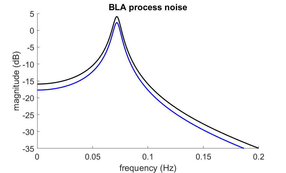
Figure 7: Dependency of the BLA on the process noise: the BLA is computed analytically with a process noise standard deviation $\sigma_{n_{x}}$ of 0.1 (blue) and 1 (black), while the input standard deviation $\sigma_{u}$ is fixed equal to 1. A clear gain increase can be observed.

Note that the chosen definition of the process noise contribution $y_{p}$ and the output noise contribution $y_{n}$ are not unique (see eq. (29) and (33)). An alternative set of definitions $\check{y}_{p}$ and $\check{y}_{n}$ could be to assign all the noise terms depending on the input $u$ to the process noise contribution, and assign all the noise terms independent of the input $u$ to the output noise contribution, resulting in the following expressions for $\check{y}_{p}$ and $\check{y}_{n}$ in this example:

$$\check{y}_{p}(t) =S(q)\left[0.3u(t)^{2}n_{x}(t)+0.3u(t)(n_{x}(t)^{2}-\sigma_{n_{x}}^{2})\right],$$

$$\check{y}_{n}(t) =n_{y}(t)+S(q)\left[n_{x}(t)+0.1n_{x}(t)^{3}\right].$$ (69)

However, the original definitions have the merit of being simple extension of the definitions used in the output noise open-loop and closed-loop setting, based on taking the expected value with respect to the output noise $n_{y}$ and the process noise $n_{x}$. Note as well that with the chosen definitions the output noise contribution only contains terms due to the output noise, while this is not the case using the alternative definition. For these reasons the authors have chosen to use the definitions that are expressed in eq. (29) and (33).

6.3 Robust Method Results

This section illustrates how the robust method can be used to estimate the BLA in a process noise setting. The experimentally obtained BLA, total variance and noise variance are compared with the analytically derived total and noise variance. Note that the robust approach does not require any knowledge of the system, while a full knowledge of the system and the (noise) signals distribution is required for the analytical derivation. A total of $M=10$ realizations is used, each containing 2 steady-state periods of 4096 points per period. The standard deviation of the input signal and noise signals are $\sigma_{u}=1$, $\sigma_{n_{x}}=0.1$ and $\sigma_{n_{y}}=0.03$.

The BLA $\hat{G}_{bla}(j\omega)$ and the variances $\hat{\sigma}_{bla,t}^{2}(j\omega)$, $\hat{\sigma}_{bla,n}^{2}(j\omega)$ obtained with the robust BLA estimation method coincide perfectly with their analytical counterparts as can be seen in Figure 8. Note that the robust approach cannot distinguish between the process noise and the output noise variance, what is shown here is the total variance of the BLA due to both the process noise and the output noise.

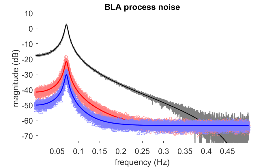
Figure 8: The estimated BLA versus the theoretically obtained BLA. The obtained BLA $G_{bla}(j\omega)$ is shown in black (analytical) and gray (robust method), the total variance on the estimated BLA is shown in light (robust method) and dark (analytical) red, while the noise variance is shown in light (robust method) and dark (analytical) blue. A good match between the analytical BLA expression and the one obtained experimentally using the robust method can be observed.

7 Conclusion

The Best Linear Approximation framework is extended to the process noise case, both for the open-loop and the closed-loop setting. The process noise acts as a second input of a Volterra system, resulting in a very general process noise framework. It is proven that the stochastic nonlinear contributions and the process noise contribution are zero-mean and uncorrelated with the input. It is also illustrated that the BLA can depend of the properties on the process noise, and that both the process noise contribution and the stochastic nonlinear distortion are uncorrelated but not independent of the input excitation. The Best Linear Approximation, together with the total and the noise variance can be obtained using the robust estimation method in the case of process noise.

This work was supported in part by the Fund for Scientific Research (FWO-Vlaanderen), the Methusalem grant of the Flemish Government (METH-1), by the Belgian Government through the Inter university Poles of Attraction IAP VII/19 DYSCO program, and the ERC advanced grant SNLSID, under contract 320378. Maarten Schoukens is supported by the H2020 Marie Sklodowska-Curie European Fellowship. The project leading to this application has received funding from the European Union’s Horizon 2020 research and innovation programme under the Marie Sklodowska-Curie grant agreement Nr 798627.

References

- Boyd and Chua [1985] S. Boyd and L.O. Chua. Fading Memory and the Problem of Approximating Nonlinear Operators with Volterra Series. IEEE Transactions on Circuits and Systems, 32(11):1150–1161, 1985.
- Bussgang [1952] J.J. Bussgang. Cross-correlation functions of amplitude-distorted Gaussian signals. Technical Report 216, MIT Laboratory of Electronics, 1952.
- Enqvist [2005] M. Enqvist. Linear Models of Nonlinear systems. PhD thesis, Institute of technology, Linköping University, Sweden, 2005.
- Enqvist [2010] M. Enqvist. Identification of Block-oriented Systems Using the Invariance Property. In F. Giri and E.W. Bai, editors, Block-oriented Nonlinear System Identification, volume 404 of Lecture Notes in Control and Information Sciences, pages 147–158. London, Berlin Heidelberg, 2010.
- Enqvist and Ljung [2005] M. Enqvist and L. Ljung. Linear approximations of nonlinear FIR systems for separable input processes. Automatica, 41(3):459–473, 2005.
- Giordano and Sjöberg [2016] G. Giordano and J. Sjöberg. Consistency aspects of Wiener-Hammerstein model identification in presence of process noise. In 55th IEEE Conference on Decision and Control (CDC), pages 3042–3047, 12 2016.
- Hagenblad et al. [2008] A. Hagenblad, L. Ljung, and A. Wills. Maximum likelihood identification of Wiener models. Automatica, 44(11):2697–2705, 2008.
- Ljung [2001] L. Ljung. Estimating Linear Time-invariant Models of Nonlinear Time-varying Systems. European Journal of Control, 7(2-3):203–219, 2001.
- Paduart et al. [2010] J. Paduart, L. Lauwers, J. Swevers, K. Smolders, J. Schoukens, and R. Pintelon. Identification of nonlinear systems using polynomial nonlinear state space models. Automatica, 46(4):647–656, 2010.
- Pintelon and Schoukens [2002] R. Pintelon and J. Schoukens. Measurement and modelling of linear systems in the presence of non-linear distortions. Mechanical Systems and Signal Processing, 16(5):785–801, 2002.
- Pintelon and Schoukens [2012a] R. Pintelon and J. Schoukens. System Identification: A Frequency Domain Approach. Wiley-IEEE Press, Hoboken, New Jersey, 2nd edition, 2012a.
- Pintelon and Schoukens [2012b] R. Pintelon and J. Schoukens. The best linear approximation of nonlinear systems operating in feedback. In IEEE International Instrumentation and Measurement Technology Conference (I2MTC), pages 2092–2097, 5 2012b.
- Pintelon and Schoukens [2013] R. Pintelon and J. Schoukens. FRF Measurement of Nonlinear Systems Operating in Closed Loop. IEEE Transactions on Instrumentation and Measurement, 62(5):1334–1345, 2013.
- Schetzen [1980] M. Schetzen. The Volterra and Wiener Theories of Nonlinear Systems. Wiley, New York, 1980.
- Schoukens et al. [1998] J. Schoukens, T. Dobrowiecki, and R. Pintelon. Parametric and non-parametric identification of linear systems in the presence of nonlinear distortions. A frequency domain approach. IEEE Transactions on Automatic Control, 43(2):176–190, 1998.
- Schoukens et al. [2009] J. Schoukens, J. Lataire, R. Pintelon, G. Vandersteen, and T. Dobrowiecki. Robustness Issues of the Best Linear Approximation of a Nonlinear System. IEEE Transactions on Instrumentation and Measurement, 58(5):1737–1745, 2009.
- Schoukens et al. [2012] J. Schoukens, R. Pintelon, and Y. Rolain. Mastering System Identification in 100 Exercises. John Wiley & Sons, Hoboken, New Jersey, 2012.
- Schoukens et al. [2015] J. Schoukens, R. Pintelon, Y. Rolain, M. Schoukens, K. Tiels, L. Vanbeylen, A. Van Mulders, and G. Vandersteen. Structure discrimination in block-oriented models using linear approximations: A theoretic framework. Automatica, 53:225–234, 2015.
- Schoukens et al. [2016] J. Schoukens, M. Vaes, and R. Pintelon. Linear System Identification in a Nonlinear Setting: Nonparametric Analysis of the Nonlinear Distortions and Their Impact on the Best Linear Approximation. IEEE Control Systems, 36(3):38–69, 2016.
- Schoukens [2017] M. Schoukens. Block-Oriented Identification using the Best Linear Approximation: Benefits and Drawbacks. In 24th DMIS Minisymposium, pages 74–77, Budapest, Hungary, 2017.
- Schoukens and Tiels [2017] M. Schoukens and K. Tiels. Identification of block-oriented nonlinear systems starting from linear approximations: A survey. Automatica, 85:272–292, 2017.
- Vaes et al. [2015] M. Vaes, J. Schoukens, B. Peeters, J. Debille, T. Dossogne, J.P. Noël, and G. Kerschen. Nonlinear ground vibration identification of an F-16 aircraft. Part I: fast nonparametric analysis of distortions in FRF measurements. In 16th International Forum on Aeroelasticity and Structural Dynamics (IFASD), Saint Petersburg, Russia, 6 2015.
- Vlaar et al. [2017] M. Vlaar, T. Solis-Escalante, A. Vardy, F. Van der Helm, and A. Schouten. Quantifying Nonlinear Contributions to Cortical Responses Evoked by Continuous Wrist Manipulation. IEEE Transactions on Neural Systems and Rehabilitation Engineering, 25(5):481–491, 2017.
- Wellstead [1977] P.E. Wellstead. Reference signals for closed-loop identification. International Journal of Control, 26(6):945–962, 1977.
- Wellstead [1981] P.E. Wellstead. Non-parametric methods of system identification. Automatica, 17(1):55–69, 1981.
- Wong et al. [2012] H.K. Wong, J. Schoukens, and K. Godfrey. Analysis of Best Linear Approximation of a Wiener-Hammerstein System for Arbitrary Amplitude Distributions. IEEE Transactions on Instrumentation and Measurement, 61(3):645–654, 2012.
- Zhang et al. [2017] E. Zhang, M. Schoukens, and J. Schoukens. Structure Detection of Wiener-Hammerstein Systems With Process Noise. IEEE Transactions on Instrumentation and Measurement, 66(3):569–576, 2017.