Phase diagram of dipolar-coupled XY moments on disordered square lattices

Abstract

The effects of dilution disorder and random-displacement disorder are analyzed for dipolar-coupled magnetic moments confined in a plane, which were originally placed on the square lattice. In order to distinguish the different phases, new order parameters are derived and parallel tempering Monte Carlo simulations are performed for a truncated dipolar Hamiltonian to obtain the phase diagrams for both types of disorder. We find that both dilution disorder and random-displacement disorder give similar phase diagrams, namely disorder at small enough temperatures favors a so-called microvortex phase. This can be understood in terms of the flux closure present in dipolar-coupled systems.

I Introduction

In frustrated magnetic systems, there is a variety of interesting phenomena including the inhibition of long-range order Wannier (1950), highly degenerate ground states Pauling (1935), incommensurate phases Elliott (1961); Fisher and Selke (1980); Selke (1988), spin glass physics Edwards and Anderson (1975); Sherrington and Kirkpatrick (1975) and emergent rules on local fluctuations Ramirez et al. (1999); Castelnovo et al. (2008). In many of these systems, including the pyrochlores Harris et al. (1997); Ramirez et al. (1999), dipolar contributions are important. Moreover, the dipolar interaction itself may be understood in terms of frustration. Here the ferromagnetic and antiferromagnetic components compete, resulting in its anisotropic behavior.

In recent years, artificial spin systems, manufactured by assembling single-domain nanoscale magnets have been investigated Heyderman and Stamps (2013); Nisoli et al. (2013); Marrows . These nanomagnets interact purely via magnetostatic coupling that, to lowest order, can be described by dipolar coupling only. In many of these artificial spin systems, the nanomagnets have Ising-like degrees of freedom Wang et al. (2006); Heyderman and Stamps (2013); Farhan et al. (2013); Cumings et al. (2014); Anghinolfi et al. (2015); Sendetskyi et al. (2016). In addition, a modification of the interaction energies was recently demonstrated by combining Ising-like nanomagnets with nanomagnets featuring continuous in-plane moments placed at the vertices Östman et al. (2018).

Systems entirely built out of dipolar-coupled moments that rotate freely in the plane are predicted to exhibit interesting physics such as continuously degenerate ground states Belobrov et al. (1983) and order-by-disorder mechanisms Prakash and Henley (1990). Their experimental investigation is, however, still in its infancy Heyderman et al. (2004); Arnalds et al. (2014); Velten et al. (2017); Leo et al. (2018). Such a system will henceforth be denoted as a dXY system, where the XY is in analogy to the XY model and the d refers to the dipolar coupling.

Without any assumptions about the geometry of a dXY system, the only symmetry supported by the Hamiltonian is time reversal. If the moments are placed on a regular lattice, the symmetry group of the Hamiltonian is enhanced by the point group of the lattice as a result of the anisotropy of the dipolar interaction. Therefore, different geometries will give rise to additional phases and universality classes for the transitions involved.

If the dXY system is placed on the square lattice, the system is known to have a continuously-degenerate ground state, despite the symmetry group of the Hamiltonian being finite rather than continuous Belobrov et al. (1983). In previous work, the so called order-by-disorder transition was demonstrated Prakash and Henley (1990). Here finite temperature leads to an effective selection of certain states of the ground-state manifold due to different spin-wave stiffnesses along certain directions that follow the fourfold symmetry of the square lattice. This results in a low-temperature long-range ordered striped phase. A similar selection effect is seen with the introduction of disorder in the form of vacancies. Here a long-range ordered microvortex state emerges, that also respects the finite symmetry of the Hamiltonian Prakash and Henley (1990).

For the non-disordered dXY system on the square lattice, the resulting phase transition to a high-temperature paramagnetic regime has been studied numerically, revealing either an Ising Baek et al. (2011) or an XYh4 De’Bell et al. (1997); Carbognani et al. (2000); Fernández and Alonso (2007) universality class transition. The critical exponents obtained by numerical investigations lie within the numerical error at the values expected for the Ising model. But, since the XYh4 has a marginal operator, which means that the critical exponents can be tuned to the critical exponents of the Ising universality class in one of the limiting cases José et al. (1977), it is not clear if the dXY system on the square lattice saturates this limit and therefore belongs to the Ising universality class, or is just close to saturation and is therefore only properly described by an XYh4 universality class. Consequently, numerical investigations of this transition are to a certain degree inconclusive.

It can, however, conclusively be argued that the value of $h_{4}$ is large De’Bell et al. (1997); Carbognani et al. (2000); Fernández and Alonso (2007), such that the system has a strong effective anisotropy, that follows the fourfold anisotropy of the square lattice. This drives the dXY system on the square lattice away from the Berezinskii-Kosterlitz-Thouless transition Berezinskii (1971); Kosterlitz and Thouless (1973) towards a clear second order phase transition.

The dilution-disordered system, where vacancies are introduced, was previously studied using a temperature-sweep Monte Carlo approach and an observable, which consisted of fourth powers of the spin components De’Bell et al. (1997); Patchedjiev et al. (2005); LeBlanc et al. (2006). Various values of dilution were examined and well-converged results were obtained up to a dilution rate of approximately $6\%$. In addition, the results qualitatively agreed with the predictions from the spin-wave analysis Prakash and Henley (1990).

The dXY system on the square lattice with random displacement of the sites was studied using a parallel tempering approach Alonso and Allés (2011). Here the spin glass overlap observable was considered and it was concluded that no spin glass phase is observed even for the highest amounts of disorder. In addition, fully random placement of dipolar-coupled XY spins, as well as random-displacement disorder applied to the square lattice, was studied by means of a saddle-point analysis Pastor and Jensen (2008). Here, it was demonstrated that a spatial localization of magnetic excitations occurs in systems with strong disorder. To the best of our knowledge, however, no phase diagram has been determined for a random-displacement disordered dXY system on the square lattice.

In this paper, the full phase diagrams for both the dilution disordered as well as the random-displacement disordered case are obtained numerically. Both diagrams display a pocket at low temperature and moderate disorder where the microvortex phase dominates. Furthermore, there is a striped phase region for smaller disorder and higher temperature. Starting from either phase, the paramagnetic regime is obtained if either temperature or disorder are increased sufficiently. The structure of the phase diagram can be understood by considering the magnetic flux closure present in dipolar systems. If the full symmetry of the square lattice is present, the flux closure can occur globally and the striped phase will dominate over the microvortex phase due to a smaller spin-wave stiffness. If the point group symmetries are broken by introduction of disorder, magnetic flux closure will occur locally and the microvortex phase will dominate at low temperatures.

The remainder of the paper is organized as follows. The model and the order parameters are introduced in section II. The methods are specified in section III and numerical data are reported for the non-disordered case in section III.1. Our results for the dilution-disordered dXY system are presented in section III.2 and for random displacement in section III.3. A Binder cumulant analysis is introduced and consequently applied to the data in order to give a system-size independent phase diagram. The limitations and the applicability of the order parameters are then discussed in section IV, where it is shown that, for the disorder range dealt with in this paper, the order parameters are still well defined. Finally, similarities between the phase diagrams for the two types of disorder are highlighted in section V and a possible interpretation of these similarities in terms of magnetic flux closure is provided.

II Model & Order Parameters

The (classical) Hamiltonian of the dXY system is given by

$$H=\frac{D}{2}\sum_{i\neq j}\frac{p_{i}p_{j}}{r_{ij}^{3}}\left[\vec{S}_{i}\cdot\vec{S}_{j}-3\left(\vec{S}_{i}\cdot\hat{r}_{ij}\right)\left(\vec{S}_{j}\cdot\hat{r}_{ij}\right)\right],$$ (1)

where the spins, as well as their positions, are confined to the $xy$-plane. $D$ denotes the dipolar-interaction strength and without loss of generality is set to $1$. The dilution parameters $p_{i}$ are either $1$ or $0$, and are 0 if the $i$th moment is removed and 1 otherwise. In the non-disordered system all $p_{i}$ are $1$. The difference vector between the positions at the sites $i$ and $j$ is denoted by $\vec{r}_{ij}$, its length by $r_{ij}$ and the normalization of this vector to unit length is denoted as $\hat{r}_{ij}$. For a non-disordered system, all sites lie on a regular square lattice in the $xy$-plane, and the nearest-neighbor distance is set to $1$. For the introduction of random displacements, the position of each site is randomly displaced in the $xy$-plane according to a Gaussian distribution.

For the remainder of the paper, a cutoff radius will be applied to the evaluation of Eq. (1) in order to speed up the calculations. Therefore instead of a summation of all sites $i\neq j$, we will only consider contributions of sites with $1\leq|\vec{r}_{ij}|\leq r_{\text{cut}}$, where $r_{\text{cut}}$ is the cutoff radius. The cutoff chosen for the simulations in section III was $r_{\text{cut}}=2$, which included the 12 closest lattice sites. In what follows, we will abbreviate the studied system with tdXY for truncated dipolar XY. The rather small value for $r_{\text{cut}}$ was chosen, since we expect that the qualitative features in the phase diagram will already be captured correctly, while the Hamiltonian can still be evaluated quickly so that extensive simulations can be performed. Note, however, that a larger value of $r_{\text{cut}}$ would result in more frustration, so that quantitative features such as the critical temperature $T_{c}$ are expected to decrease with larger $r_{\text{cut}}$.

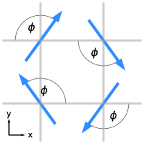
(a)

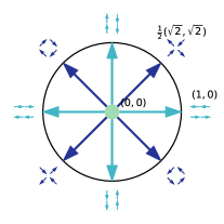
(b)

Figure 1: (color online) (a) The degenerate ground state of the square-lattice dXY system is defined within a two-by-two magnetic unit cell via an angle-degeneracy parameter $\phi$. (b) Possible vectors $\vec{M}$ are shown as given in Eq. (2). The black solid circle indicates $|\vec{M}|=1$, which is fulfilled for the ground state manifold depicted in (a). The arrows correspond to the four striped phases (light blue) and the four microvortex phases (dark blue). A pictograph is given to associate the vectors with their respective phases. The light blue dot in the middle corresponds to the paramagnetic phase.

Irrespective of a truncation of the summation in Eq. (1), the ground state of the dXY system on the square lattice is continuously degenerate and is defined in the magnetic unit cell, which is a two-by-two plaquette. The ground state spin configuration is parametrized by a global angle-degeneracy parameter $\phi$, as depicted in Fig. 1a Belobrov et al. (1983). This continuous degeneracy is broken by finite temperature or dilution disorder as shown in Ref. Prakash and Henley (1990). Namely, thermal excitations favor striped phases, where $\phi=n\frac{\pi}{2}$ for $n\in\mathbb{Z}$, due to different spin-wave stiffnesses along different directions. In contrast to thermal excitations, dilution disorder is known to select the so-called microvortex phase, where $\phi=\frac{\pi}{4}+n\frac{\pi}{2}$ again with $n\in\mathbb{Z}$. The microvortex phase ensures magnetic flux closure at the scale of each plaquette, whereas magnetic flux closure happens in the striped phase at infinity.

Up to now De’Bell et al. (1997); Carbognani et al. (2000); Rastelli et al. (2002); Fernández and Alonso (2007); Baek et al. (2011), any type of long range order in the dXY or the tdXY systems on the square lattice has been described with the magnitude of the order parameter

$$|\vec{M}| =\frac{1}{N}\left|\sum_{i}\left(\left(-1\right)^{y_{i}}\cos\theta_{i},\left(-1\right)^{x_{i}}\sin\theta_{i}\right)\right|,$$ (2)

where $\theta_{i}$ is the angle of the $i$th spin with, for example, the $x$-axis. The sites are enumerated with $x_{i}$ and $y_{i}$ along $\hat{x}$ and $\hat{y}$. In the non-disordered case, under the assumption of a nearest-neighbor distance of $1$, the enumeration indices $x_{i}$ and $y_{i}$ are also the $x$ and $y$ coordinates respectively. The order parameter is normalized to be $1$ for the ground states by dividing by the total number of spins $N$. The vector $\vec{M}$ lies on the unit circle for the ground state configurations. Possible values for the vector $\vec{M}$ are depicted in Fig. 1b and example ground states are given as pictographs, which represent the character of the phase given by each vector. As an example, the point $(1,0)$ corresponds to a striped order along $\hat{x}$, whereas $(-1,0)$ also corresponds to a striped order along $\hat{x}$ shifted by half a magnetic unit cell along the $\hat{y}$ direction. Analogously, striped orders along $\hat{y}$ correspond to the two vectors $(0,\pm 1)$. The microvortex phases correspond to the four points at $\frac{1}{\sqrt{2}}(\pm 1,\pm 1)$ and the paramagnetic phase corresponds to $(0,0)$.

Since the vector $\vec{M}$ lies on the circle described by $|\vec{M}|=1$ for all ground state phases, it is not possible to distinguish the microvortex phase from the striped phase by the magnitude $|\vec{M}|$. However, it is possible to differentiate between the paramagnetic phase and long-range order in either the microvortex phase or the striped phase.

In order to differentiate the ground state phases, we can consider the polar representation of the order parameter $\vec{M}=(M_{x},M_{y})=|\vec{M}|(\cos\phi,\sin\phi)$. The vector with doubled angle ($|\vec{M}|(\cos 2\phi,\sin 2\phi)$) is introduced since this vector assigns the striped phases to vectors along the $x$-axis and the microvortex phases to vectors along the $y$-axis. This gives:

$$|\vec{M}|\cos\left(2\arctan\left(\frac{M_{y}}{M_{x}}\right)\right) =\frac{M_{x}^{2}-M_{y}^{2}}{|\vec{M}|},$$ (3a)

$$|\vec{M}|\sin\left(2\arctan\left(\frac{M_{y}}{M_{x}}\right)\right) =\frac{2M_{x}M_{y}}{|\vec{M}|},$$ (3b)

which describe the projections of a state onto its striped phase components and its microvortex phase components, respectively.

Eqs. (3) therefore give possible order parameters for (a) the striped and (b) the microvortex phase. These order parameters are, however, numerically unfavorable at high temperature, since they are divided by the length of the vector $|\vec{M}|$. Group theory can therefore be considered in order to find order parameters with the same transformation properties. Such order parameters have to transform as irreducible representations of the symmetry group of the underlying system. For the dXY model on the square lattice, the symmetry group is given by time reversal symmetry enhanced by the corresponding point group of the lattice, which is $C_{4v}$ for the square lattice. The character table for this point group is given in Table 1. In the last column of the table, the simplest functions are indicated, which transform according to the irreducible representations. These functions are the symmetry-allowed combinations of the components of the vector $\vec{M}$ used to construct the order parameters.

Table 1: Character table for $C_{4v}$, the point group of the square lattice.

$C_{4v}$	$E$	$2C_{4}$	$C_{2}$	$2\sigma_{v}$	$2\sigma_{d}$
$A_{1}$	$1$	$1$	$1$	$1$	$1$	$x^{2}+y^{2}$
$A_{2}$	$1$	$1$	$1$	$\overline{1}$	$\overline{1}$
$B_{1}$	$1$	$\overline{1}$	$1$	$1$	$\overline{1}$	$x^{2}-y^{2}$
$B_{2}$	$1$	$\overline{1}$	$1$	$\overline{1}$	$1$	$xy$
$E$	$2$	$0$	$\overline{2}$	$0$	$0$	$(x,y)$

The vector $\vec{M}$ itself transforms according to the irreducible representation $E$, and therefore serves as an order parameter. The length of the vector transforms according to the trivial representation $A_{1}$ that, due to its transformation property, can only be used to distinguish between long-range order and the paramagnetic phase. Inspection of Table 1 reveals that the two projections derived in Eqs. (3a) and (3b) transform according to the irreducible representations $B_{1}$ and $B_{2}$, respectively, and therefore serve as valid order parameters.

Thus,

$$M_{{s}}=\sqrt{|M_{x}^{2}-M_{y}^{2}|}\quad\text{and}\quad M_{{mv}}=\sqrt{|2M_{x}M_{y}|}$$ (4)

are also valid order parameters for the striped phase and the microvortex phase, since they transform according to $B_{1}$ and $B_{2}$ respectively. Furthermore, $M_{s}$ and $M_{mv}$ are numerically more stable as they do not contain a division by the magnitude $|\vec{M}|$. These two quantities as well as $|\vec{M}|$ are determined in the subsequent Monte Carlo simulations in order to distinguish between the different phases.

III Monte Carlo Simulations

Monte Carlo simulations are now performed for the tdXY system on the square lattice in order to construct the phase diagrams for both the dilution-disordered system as well as the random-displacement disordered system. The code is based on the ALPS project Troyer et al. (1998); Albuquerque et al. (2007); Bauer et al. (2011). It uses a parallel tempering algorithm Swendsen and Wang (1986); Hukushima and Nemoto (1996); Katzgraber et al. (2006) (also known as replica-exchange Monte Carlo) in order to thermalize even quite heavily frustrated systems. Parallel tempering refers to the simulation of the same system at several temperatures in parallel, with regular exchange of the temperatures between the simulations according to a detailed-balance condition. All figures are generated with matplotlib Hunter (2007).

In the following simulations periodic boundary conditions were used. We thermalized the system with $2\cdot 10^{5}$ lattice sweeps. Subsequently, $10^{4}$ measurements were made while, between two successive measurements, 15 lattice sweeps were carried out. For the disordered cases, a total of 40 different temperatures were used, which were linearly distributed between $T=0.1$ and $T=1.6$. The simulations performed for this work took a total of approximately $10^{5}$ CPU hours, with the majority of time spend on simulating the disordered systems, where the disorder average over several realizations had to be taken. Before considering the simulations for the disordered systems the non-disordered case is first simulated to gain further insight into this simpler situation where no disorder average has to be taken.

III.1 No Disorder

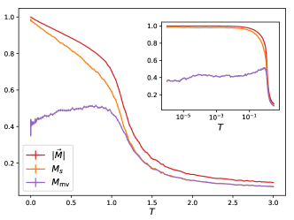
(a)

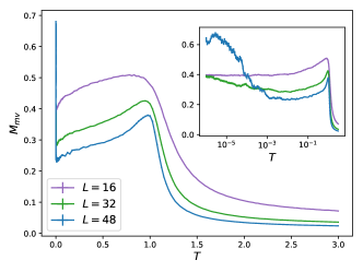
(b)

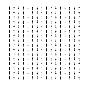
(c)

Figure 2: (color online) (a) The temperature dependence of the three order parameters discussed in section II are shown. These are obtained with parallel tempering Monte Carlo simulations for the non-disordered tdXY system with a system size of $L=16$ averaged over $4$ independent runs. The same data plotted on a logarithmic temperature scale is shown in the inset. (b) The microvortex order parameter is shown for the three system sizes studied. The same data is plotted on a logarithmic temperature scale in the inset to highlight the transition at $T=0$. (c) A configuration is shown, which was obtained by our simulations at temperature $1.8\cdot 10^{-6}$. Since the microvortex order parameter is very homogeneous across the system, it is likely to originate from the Goldstone mode.

The simulation for the non-disordered system was performed in order to validate the order parameters derived in section II. In total, 220 temperatures were implemented, which were uniformly spaced at higher temperatures and logarithmically spaced at lower temperatures. The three order parameters are plotted versus the temperature in Fig. 2a. As expected, the magnitude $|\vec{M}|$ indicates the appearance of long-range order as the temperature decreases (obtained from the Binder cumulant crossing: $T_{c}(r_{\text{cut}}=2)=0.996\pm 0.017$). A similar trend is visible for $M_{s}$. Furthermore, fluctuations away from the striped phase have a contribution to $M_{mv}$, so that $M_{mv}$ rises around the phase transition between the paramagnetic phase and the striped phase and then slowly decays.

In the inset of Fig. 2a, we show the same data with a logarithmic temperature axis. The value of $M_{mv}$ appears to saturate at around $0.4$. Comparing, however, with Fig. 2b, where the data for $M_{mv}$ is shown for three different system sizes it can be seen that there is a steep increase of $M_{mv}$, which indicates the transition to the angle degenerate ground state Prakash and Henley (1990). This transition is driven by the Goldstone mode, which is a result of the angle degenerate ground state, transforming in this case $\phi\rightarrow\phi+\delta\phi$ in Fig. 1a over a large length scale. This Goldstone mode can be seen in Fig. 2c, where $M_{mv}$ is distributed very homogeneously across the system. Note that the Goldstone mode makes all angles $\phi$ in Fig. 1a equally accessible, so that the saturation value for $M_{mv}$ in the limit $T\rightarrow 0$ can be computed as an average with respect to $\phi$. Doing so gives $M_{mv}\approx 0.7628$ for $T\rightarrow 0$, which is consistent with the trend seen in the inset of Fig. 2b for the largest system size considered.

To conclude the results of this section, the order parameters $M_{s}$ and $M_{mv}$ introduced in Eq. (4) give a measure of the striped phase and the microvortex phase respectively. Therefore they can be used in the subsequent simulations in the two disordered cases to obtain the phase diagrams of the tdXY systems.

III.2 Dilution

We now consider dilution disorder through the introduction of vacancies. Starting with the non-disordered square lattice, moments are removed with a probability $p$, which will be referred to as the dilution rate.

The diluted square-lattice dXY was previously treated using a spin-wave calculation in order to obtain the phase diagram Prakash and Henley (1990). In this spin-wave calculation a truncation of $r_{\text{cut}}=1$ was applied. For small but finite $p$ at $T=0$, the microvortex phase is preferred and for small but finite $T$ at $p=0$, the striped phase is preferred. For any value of $p$ at sufficiently high $T$, the paramagnetic phase is expected. With temperature-sweep Monte Carlo simulations, a first quantitative phase diagram was constructed De’Bell et al. (1997); Patchedjiev et al. (2005); LeBlanc et al. (2006). Here, the measured observable consisted of fourth powers of the spin components and essentially was a measure of the likelihood that spins point along diagonals rather than along axes. This gave an indication of the selected phase, but did not serve as an order parameter. This led to well-converged results for small values of $p$. However, due to the frustration and the disorder at higher values of the dilution rate, a temperature-sweep algorithm is prone to get stuck in metastable states, so that no conclusive statement was possible above a dilution rate of approximately $6\%$.

The order parameters determined by our Monte Carlo simulations as a function of temperature and dilution rate are summarized in Fig. 3. There is good convergence of the data for all system sizes, temperatures and dilution rates since there is no visible noise. The previously proposed phase diagram Prakash and Henley (1990) is in qualitative agreement with the results for $M_{s}$ and $M_{mv}$. Namely, there is a pocket at low temperatures and finite dilution rate where the microvortex phase is predominant (region with strong signal in the panels for $M_{mv}$, which is more visible at larger system sizes). In addition, for small dilution rates and high enough temperatures, the striped phase dominates (region with a strong signal in the panels for $M_{s}$). Nonetheless, in regions where one phase dominates, there is still some signal of the order parameter for the other phase visible. This occurs because fluctuations from one phase appear as an increase in the order parameter of the other phase.

Previously, it was predicted for a nearest-neighbor truncated dipolar Hamiltonian Prakash and Henley (1990) that any long-range order disappears close to the percolation limit of the square lattice at $1-p_{c}^{\text{perc}}=40.7\%$. This is in agreement with the general expectation for nearest-neighbor only Hamiltonians, that no long-range order can be seen above the percolation threshold. However, inspection of $|\vec{M}|$ in Fig. 3 reveals that there is no longer a sizable contribution to the long-range order parameter already at a dilution rate of $p_{c}(r_{\text{cut}}=2)\approx 15\%$. Note that this value is dependent on the cutoff and that the inclusion of more lattice sites leads to a reduction of both $T_{c}$ as well as $p_{c}$ due to the increase in frustration present in the system. This is in contrast to percolation theory, which predicts an increase of $p_{c}$ as $r_{\text{cut}}$ is increased.

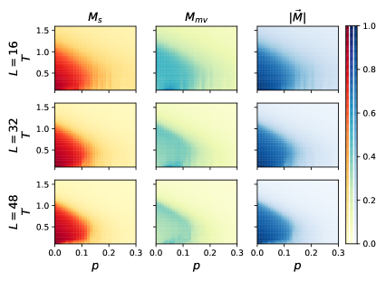
Figure 3: (color online) Each of the order parameters for the dilution-disordered tdXY system on the square lattice as a function of dilution rate $p$ and temperature $T$ for three different system sizes ($L=16,32,48$) obtained via parallel tempering Monte Carlo simulations averaged over 32 disorder realizations.

All of the data presented in Fig. 3 is system-size dependent. In order to give a system-size independent phase diagram another method needs to be implemented. Even though the data is not good enough to attempt a scaling collapse, a Binder cumulant analysis can be applied. Crossings of the cumulants for different system sizes at a fixed dilution rate can, up to corrections to scaling, precisely locate the critical temperatures for the involved transitions.

Making use of the binning analysis implemented in ALPS, we obtain the Binder cumulants with their statistical error. Through a resampling procedure, such error information can be used to obtain possible realizations of the Binder cumulant curves. In particular, the mean value of the Binder cumulants as a function of $T$ at a fixed value of $p$ was perturbed with uncorrelated Gaussian noise according to the statistical error at each sampling point. Through the analysis of many such curves, statistics on the crossings can be obtained and, from this, an estimate for $T_{c}$ and its uncertainty at every value of $p$ can be determined. We refer to this method as the fixed dilution rate analysis. Analogously, the same procedure can be applied for the Binder cumulants at a fixed temperature as a function of $p$ in order to obtain an estimate for $p_{c}$ at every value of $T$. We refer to this as the fixed temperature analysis.

The system-size independent phase diagram is shown in Fig. 4. Filled markers denote the procedure where the data was analyzed for a fixed dilution rate to obtain $T_{c}$, whereas open markers are the data for $p_{c}$ obtained with the fixed temperature analysis. The Binder cumulant estimate for $T_{c}$ ($p_{c}$) are shown with red dots, violet diamonds and orange triangles for $|\vec{M}|$, $M_{mv}$ and $M_{s}$, respectively. For comparison, the microvorticity heat map ($M_{mv}$) for $L=48$ is shown in the background.

A few remarkable features can be identified in Fig. 4. At the critical line separating the paramagnetic phase and the striped phase, $T_{c}$ predicted by the Binder cumulant analysis of $M_{s}$ and $|\vec{M}|$ agree well and have small error bars. This data also agrees well with the data for $p_{c}$, which was obtained by the fixed temperature analysis. Furthermore, the fixed temperature analysis yielded the boundary between the striped phase and the paramagnetic phase at $p_{c}(T=0,r_{\text{cut}}=2)\approx 11\%$, a value which is system size independent, in contrast to the earlier estimate of 15%. Note that $p_{c}$ is cutoff dependent. Since a larger $r_{\text{cut}}$ increases the frustration, we expect that $p_{c}(T=0,r_{\text{cut}}=\infty)\leq p_{c}(T=0,r_{\text{cut}}=2)$, so that our result for $p_{c}$ serves as an upper bound to $p_{c}(r_{\text{cut}}=\infty)$. In fact, the frustration could even lead to $p_{c}(r_{\text{cut}}\to\infty)\to 0$.

At $p>11\%$, our fixed dilution rate analysis could no longer provide quantitative data. This is due to the fact that the phase boundary is close to vertical, so that $T_{c}$ in this area is very sensitive to $p$. At the lower critical line, separating the microvortex phase (region “mv”) from the striped phase (region “s”), there is again good agreement between the data for the Binder cumulants of $M_{mv}$ and $M_{s}$. However, here the error bars are substantially larger. This is due to the Binder cumulants being flatter as a function of temperature, resulting in poorly defined crossings. The fixed temperature analysis did not perform well for the phase boundary between the microvortex phase and the striped phase since it was noise dominated. Therefore this data is not shown. At $p\geq 12\%$, the analysis could no longer be performed, as there were no more crossings. This corresponds to the onset of paramagnetism in the region labeled “para”.

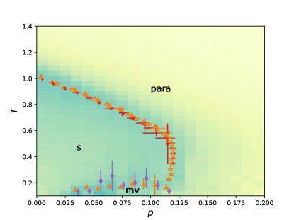
Figure 4: (color online) The phase diagram for the diluted square lattice tdXY system as a function of dilution rate and temperature derived via Binder cumulant crossings, superimposed on the corresponding $M_{mv}$ data of Fig. 3 for $L=48$. The filled (open) markers give $T_{c}$ ($p_{c}$) with red dots for $|\vec{M}|$, orange triangles for $M_{s}$ and violet diamonds for $M_{mv}$ respectively. Region “mv” corresponds to the microvortex phase, region “s” to the striped phase and region “para” to the paramagnetic phase.

III.3 Random displacement

We now introduce random displacement. Starting with the non-disordered square lattice, every site is relocated by a random displacement in the $xy$-plane, taken from a Gaussian random distribution with standard deviation $\sigma$.

To the best of our knowledge, no attempt has been made to provide a phase diagram with respect to the strength of the random displacement, even though simulations have been performed for both medium disorder Alonso and Allés (2011) and strong disorder given by random placement of the moments Pastor and Jensen (2008). For the work on medium disorder Alonso and Allés (2011) the starting point was the square lattice and random displacements taken from a Gaussian distribution were introduced. This paper was mainly concerned with the disappearance of long-range order with the appearance of a possible spin glass phase for higher values of disorder. The random placement of moments Pastor and Jensen (2008) resulted in a spatial localization of magnetic excitations as well as low-energy states incorporating microvortex-like structures. The scope of this work was, however, mainly the low-energy excitations and not the construction of the phase diagram.

Our results for the three order parameters are shown in Fig. 5a. Similar to the dilution-disordered case, for random-displacement disorder, the system also favors the microvortex phase at low temperatures with a pocket of large values of the microvortex order parameter for small $T$ and intermediate $\sigma$. Likewise, a high enough temperature results in the striped phase (small $\sigma$ and intermediate $T$). Analogous to the dilution-disordered case presented in section III.2, the heat maps for $|\vec{M}|$ indicate where no sizable contribution to long-range order is expected, which occurs at approximately $\sigma>0.12$.

While the phase diagrams in Fig. 4 and 5b are for two different types of disorder, they should agree at $p=0$ and $\sigma=0$, since here both simulations are non-disordered. At first glance, this does not appear to be the case, but looking closely at the phase diagram of the random displacement disordered system at small $\sigma$, the data does indeed agree with the non-disordered system and behaves continuously with $\sigma$. However, even small values of $\sigma\lesssim 0.01$ are sufficient to stabilize the microvortex phase up to considerably high temperatures, which explains the apparent mismatch between the two figures.

As carried out for the dilution-disordered system, a Binder cumulant analysis was performed for the random-displacement disordered system. The results are displayed in Fig. 5b, where again the microvorticity order parameter for $L=48$ is displayed in the background to serve as a reference. The definitions of the marker colors, forms and fillings for the data points of the Binder cumulant crossings are the same as for the dilution-disordered case. Again, the regions in the figure correspond to the microvortex phase (mv), the striped phase (s) and the paramagnetic phase (para). At some phase boundaries it was not possible to determine the Binder cumulant crossing for the fixed temperature analysis due to statistical noise and data points are only shown where the analysis could reliably be performed. Once more, a good agreement between the data for the different order parameters can be seen. The Binder cumulant analysis at a fixed disorder strength breaks down at a disorder strength of $\sigma_{c}(T=0,r_{\text{cut}}=2)\approx 0.06$. This is again cutoff dependent. As argued in the dilution disordered case, we expect analogously $\sigma_{c}(T=0,r_{\text{cut}}=\infty)\leq\sigma_{c}(T=0,r_{\text{cut}}=2)$. Note that non-negligible values of the microvortex parameter persist up to $\sigma\approx 0.11$, which is much larger than $\sigma_{c}(T=0,r_{\text{cut}}=2)$. The appearance of the associated region “fs” can be explained by the finite size of the simulations. Indeed, this region becomes smaller as the system size gets bigger as seen in Fig. 5a, middle column.

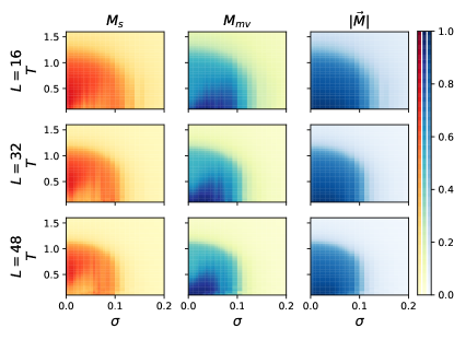
(a)

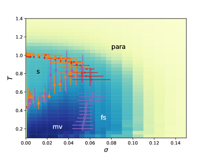
(b)

Figure 5: (color online) (a) Each of the order parameters for random-displacement disordered tdXY systems on the square lattice as a function of the width of the random displacement $\sigma$ and temperature $T$ for three different system sizes ($L=16,32,48$) obtained via parallel tempering Monte Carlo simulations averaged over 32 realizations. (b) The phase diagram of the same system as (a), as a function of temperature and width of the random displacement. This is derived via Binder cumulant crossing and superimposed on the corresponding $M_{mv}$ data for $L=48$ of (a). The assignment of colors, markers and regions is the same as in Fig. 4. The region “fs” not present in the dilution case denotes region dominated by finite size effects.

IV Applicability of the order parameters

Strictly speaking, the order parameters ($|\vec{M}|$, $M_{s}$, $M_{mv}$) are only valid for the non-disordered system, since any disorder will in principle invalidate the symmetry discussion made in section II. Nevertheless, for small disorder, the derived order parameters should still be approximately valid. The implicit assumption made to employ the derived order parameters, even in disordered systems, is that the enumeration indices $x_{i}$ and $y_{i}$ in Eq. (2) are approximately valid descriptions of the lattice positions. Certainly for small disorder the indices specify the positions well. However, in the highly disordered systems, this is no longer true.

To test if the enumeration in terms of $x_{i}$ and $y_{i}$ is valid, the random-displacement disordered system can be considered. The problem of enumeration becomes apparent when two moments exchange their relative order. This is formally written as follows: let us denote the position of the $i$th moment in the non-disordered case with $\vec{r}=(r^{x}_{i},r^{y}_{i})$ and the position after applying the disorder with $\vec{R}=(R^{x}_{i},R^{y}_{i})$. To compute the exchange probability, consider now two sites $i$ and $j$, which respect in the non-disordered case $r^{x}_{i}<r^{x}_{j}$. An exchange along the $x$-direction has occurred if $R^{x}_{i}>R^{x}_{j}$. Analogously for the $y$-direction, $r^{y}_{i}<r^{y}_{j}$ but $R^{y}_{i}>R^{y}_{j}$. The probability of an exchange event depends on the width of the random displacement and can be computed to be

$$\rho_{\text{ex}}(\sigma) =2\cdot\frac{1}{2\pi\sigma^{2}}\int_{-\infty}^{\infty}\mathrm{d}v\int_{v}^{\infty}\mathrm{d}u\>e^{-\frac{u^{2}}{2\sigma^{2}}}e^{-\frac{(v-1)^{2}}{2\sigma^{2}}}.$$ (5)

The factor $2$ comes from considering the exchange of sites along both the $x$-direction as well as the $y$-direction.

As soon as an exchange event occurs, the group theoretical symmetry discussion in section II will be invalidated. Therefore we need to make sure that the value of $\rho_{\text{ex}}(\sigma)$ is small enough, so that the order parameters obtain from the simulations are well defined in each region of the phase diagram. For example, the exchange probability given in Eq. (5) can be computed for the largest $\sigma$ used in section III.3, namely a standard deviation of $\sigma=0.2$, resulting in $\rho_{\text{ex}}(\sigma=0.2)=4\cdot 10^{-4}$. This exchange probability appears to be relatively high considering that, even in the $L=16$ system, the exchange of two sites is expected to happen a total of $3$ times in $32$ disorder realizations. Therefore in approximately $10\%$ of the simulations, the definition of the order parameter breaks down at least locally. However, this is the highest disorder considered and the system is already in the paramagnetic phase, so that an error of this size should not affect the conclusions considering the phase diagram.

For smaller values of $\sigma$, the exchange probability diminishes drastically. To illustrate this, for $\sigma=0.16$, which is just slightly smaller than the highest disorder considered, the exchange is expected to only occur once in the 32 disorder realizations for the largest considered system-size ($L=48$) and this is still deep in the paramagnetic phase. Below $\sigma=0.16$, $\rho_{\text{ex}}\approx 0$ so it is not expected that the order parameters break down at all in the simulations for low $\sigma$. Therefore, we can conclude that the order parameter definitions in Eq. (4) are well justified for the construction of the phase diagrams.

V Conclusions

In this work a truncated version of dipolar-coupled XY (tdXY) spin system on the square lattice was treated under the influence of disorder with Monte Carlo simulations. Starting from the perfect lattice, disorder was introduced in two different forms, namely by introduction of vacancies and by random displacement of each site. Some features of these systems are already known from previous work Belobrov et al. (1983); Prakash and Henley (1990); De’Bell et al. (1997); Patchedjiev et al. (2005); LeBlanc et al. (2006); Pastor and Jensen (2008); Alonso and Allés (2011); Baek et al. (2011). This paper extends these results by first deriving order parameters for the phases known as the striped phase and the microvortex phase. The order parameters of the tdXY system were then determined using parallel tempering Monte Carlo simulations, first for non-disordered systems down to very low temperatures, and then for systems with either dilution or random displacement as sources of disorder. The phase diagrams for both cases of disorder were obtained via a Binder cumulant approach, to find system-size independent values for $T_{c}$ ($p_{c}$, $\sigma_{c}$) as well as to quantify the uncertainty. Finally it was argued that the definitions of the order parameters are well defined even in the disordered systems.

The newly derived order parameters, as well as the use of parallel tempering Monte Carlo simulations, allowed us to distinguish the long-range ordered phases from the paramagnetic phase, and to determine the character of the long-range ordered phases. For both types of disorder, well-converged results for the order parameters as a function of temperature and disorder strength were obtained for all system sizes. Furthermore, the system-size independent phase diagram could be derived via a Binder cumulant analysis, which gave in most regions small error bars for $T_{c}$ as well as $p_{c}$ and $\sigma_{c}$.

In previous work on the dilution-disordered system Prakash and Henley (1990); De’Bell et al. (1997); Patchedjiev et al. (2005); LeBlanc et al. (2006), it was speculated that the disappearance of long-range order would occur close to the percolation threshold of the square lattice ($1-p_{c}^{\text{perc}}=40.7\%$). In contrast to these predictions, our simulation result for $r_{\text{cut}}=2$ showed a much lower critical dilution rate of $p_{c}(T=0,r_{\text{cut}}=2)\approx 11\%$. This value should serve at least as an upper bound on $p_{c}(r_{\text{cut}}=\infty)$.

A full phase diagram for the random-displacement disordered tdXY system on the square lattice was obtained. In contrast to the dilution-disordered system, a large region seemed to be apparent (region “fs” in Fig. 5b), where the system size results in a sizable contribution to the order parameters. This region “fs” is expected to vanish in the thermodynamic limit. Also for this system an upper bound on the critical disorder strength of $\sigma_{c}(r_{\text{cut}}=2)\approx 0.06$ was obtained, above which no long-range order is expected.

Interestingly, in the phase diagrams for both the dilution-disordered system as well as the random-displacement disordered system, the other regions behave similarly, even though the notion of disorder in the two systems is quite different. In particular, the microvortex phase is favored by both types of disorder. Also, in both systems, at high enough temperature and small enough disorder, the striped phase is favored, before ending in the paramagnetic phase at higher temperatures or disorder strengths.

These similarities in the phase diagrams suggest a general mechanism for the selection of the microvortex phase, which is common to both dilution and random displacement. This can be understood by considering the fact that in disordered systems, in contrast to the non-disordered system, it is more difficult for magnetic flux closure to occur at bulk length scales, since disorder breaks locally many of the previously available symmetries. Therefore, instead of a global magnetic flux closure obtained by the striped phase, a more local magnetic flux closure structure as in the microvortex phase is likely to be favorable. The derivation of this more general mechanism from an analytic perspective poses an interesting question for future work.

The data is openly available at http://doi.org/10.5281/zenodo.1326251