Parallel Quicksort without Pairwise Element Exchange

Abstract

Quicksort is an instructive classroom approach to parallel sorting on distributed memory parallel computers with many opportunities for illustrating specific implementation alternatives and tradeoffs with common communication interfaces like MPI. The (two) standard distributed memory Quicksort implementations exchange partitioned data elements at each level of the Quicksort recursion. In this note, we show that this is not necessary: It suffices to distribute only the chosen pivots, and postpone element redistribution to the bottom of the recursion. This reduces the total volume of data exchanged from $O(n\log p)$ to $O(n)$, $n$ being the total number of elements to be sorted and $p$ a power-of-two number of processors, by trading off against a total of $O(p)$ additional pivot element distributions. Based on this observation, we describe new, exchange-free implementation variants of parallel Quicksort and of Wagar’s HyperQuicksort.

We have implemented the discussed four different Quicksort variations in MPI, and show that with good pivot selection, Quicksort without pairwise element exchange can be significantly faster than standard implementations on moderately large problems. For smaller input sizes, standard and exchange-free variants can be combined to exploit the exchange-free variant as subproblems become large enough relative to the number of processors. On a medium sized high-performance cluster, exchange-free parallel Quicksort achieves an absolute speed-up of about 650 on $1024$ processes when sorting $10^{8}$ floating point numbers. In a weak-scaling experiment on $8192$ processes, the exchange-free variants are consistently about a factor 1.3 faster than their standard counterparts when the number of elements per process exceeds $500\,000$. The combination of standard and exchange-based variant never performs worse than either, and for a medium number of elements per process, better than both.

1 Introduction

Quicksort [6] is often used in the classroom as an example of a sorting algorithm with obvious potential for parallelization on different types of parallel computers, and with enough obstacles to make the discussion instructive. Still, distributed memory parallel Quicksort is practically relevant (fastest) for certain ranges of (smaller) problem sizes and numbers of processors [1, 2].

This note presents two new parallel variants of the Quicksort scheme: select a pivot, partition elements around pivot, recurse on two disjoint sets of elements. A distributed memory implementation needs to efficiently parallelize both the pivot selection and the partitioning step in order to let the two recursive invocations proceed concurrently. In standard implementations, partitioning usually involves exchanging elements between neighboring processors in a hypercube communication pattern. We observe that this explicit element exchange is not necessary; it suffices instead to distribute the chosen pivots over the involved processors. This leads to two new exchange-free parallel Quicksort variants with a cost tradeoff between element exchange and pivot distribution. We discuss implementations of the two variants using the Message-Passing Interface (MPI) [9], and compare these to standard implementations of parallel Quicksort. Experiments on a medium scale cluster show that this can be faster than the standard pairwise exchange variants when the number of elements per process is not too small. The two approaches can be combined for a smooth transition between exchange-based and exchange-free Quicksort.

Using MPI terminology, we let $p=2^{k}$ denote the number of MPI processes that will be mapped to physical processor(core)s. For the Quicksort variants discussed here, $p$ must be a power of two. MPI processes are ranked consecutively, $i=0,\ldots,p-1$. We let $n$ denote the total number of input elements, and assume that these are initially distributed evenly, possibly randomized [1] over the $p$ processes, such that each process has roughly $n/p$ elements. Elements may be large and complex and hence expensive to exchange between processes; but all have a key from some ordered domain with a comparison function $<$ that can be evaluated in $O(1)$ time. For each process, input and output elements are stored consecutively in process local arrays. For each process, the number of output elements should be close to the number of input elements, but actual load balance depends on the quality of the selected pivots. The output elements for each process must be sorted, and all output elements for process $i$ must be smaller than or equal to all output elements of process $i+1$, $0\leq i<p-1$.

2 Standard, distributed memory Quicksort and HyperQuicksort

Standard, textbook implementations of parallel Quicksort for distributed memory systems work roughly as follows [11, 4, 8, 15, 16]. A global pivot is chosen by some means and distributed over the processes, after which the processes all perform a local partitioning of their input elements. The processes pair up such that process $i$ is paired with process $i\oplus p/2$ (with $\oplus$ denoting bitwise exclusive or), and process pairs exchange data elements such that all elements smaller than (or equal to) the pivot end up at the lower ranked process, and elements larger than (or equal) to the pivot at the higher ranked process. After this, the set of processes is split into two groups, those with rank lower than $p/2$ and those with larger rank. The algorithm is invoked recursively on these two sets of processes, and terminates with a local sorting step when each process belongs to a singleton set of processes.

Assuming that pivots close to the median element can be effectively determined, the communication volume for the element exchange over all recursive calls is $O(n\log p)$. With linear time communication costs, the exchange time per process is $O(n/p\log p)$. Global pivot selection and distribution is normally done by the processes locally selecting a (sample of) pivot(s) and agreeing on a global pivot by means of a suitable collective operation. If we assume the cost for this to be $O(\log p+s)$ where $s,s\geq 1$, is the size of the pivot sample per process, the total cost for the pivot selection becomes $O(\log p(\log p+s))$. Some textbook implementations simply use the local pivot from some designated process which is distributed by an MPI_Bcast operation [11, 4]; others use local pivots from all processes from which a global pivot closer to the median is determined by an MPI_Allreduce-like operation [1, 14]. Either of these take time $O(\log p+s)$ in a linear communication cost model, see, e.g. [12]. Before the recursive calls, the set of MPI processes is split in two which can conveniently be done using the collective MPI_Comm_create operation, and the recursive calls simply consist in each process recursing on the subset of processes to which it belongs. Ideally, MPI_Comm_create takes time $O(\log p)$. At the end of the recursion, each process locally sorts (close to) $n/p$ elements. The best, overall running time for this parallel Quicksort implementation becomes $O(n/p\log p+n/p\log(n/p)+\log^{2}p)=O(n/p\log n+\log^{2}p)$ assuming a small (constant) sample size $s$ is used, with linear speed-up over sequential $O(n\log n)$ Quicksort when $n/p$ is in $\Omega(\log n)$. We refer to this implementation variant as standard, parallel Quicksort.

Wagar [16] observed that much better pivot selection would result by using the real medians from the processes to determine the global pivots. In this variation of the Quicksort scheme, the processes first sort their $n/p$ elements locally, and during the recursion keep their local elements in order. The exact, local medians for the processes are the middle elements in the local arrays, among which a global pivot is selected and distributed by a suitable collective operation. As above, this can be done in $O(\log p)$ time. The local arrays are split into two halves of elements smaller (or equal) and larger (or equal) than the global pivot. Instead of having to scan through the array as in the parallel Quicksort implementation, this can be done in $O(\log(n/p))$ time by binary search. Processes pairwise exchange small and large elements, and to maintain order in the local arrays, each process has to merge its own elements with those received from its partner in the exchange. The processes then recurse as explained above. The overall running time of $O(n\log n+\log^{2}p)$ is the same as for parallel Quicksort. Wagar’s name for this Quicksort variant is HyperQuicksort. Wagar [16], Quinn [10, 11], Axtmann and Sanders [1] and others show that HyperQuicksort can perform better than parallel Quicksort due to the possibly better pivot selection. A potential drawback of HyperQuicksort is that the process-local merge step can only be done after the elements from the partner process have been received. In contrast, in parallel Quicksort, the local copying of the elements that are kept at the process can potentially be done concurrently (overlapped) with the reception of elements from the partner process.

For completeness, the two standard parallel Quicksort implementation variants are shown as Algorithm 3 and Algorithm 4 in the appendix.

3 Exchange-free, parallel Quicksort

We observe that the partitioning step can be done without actually exchanging any input elements. Instead, it suffices to distribute the pivots, and postpone the element redistribution to the end of the recursion.

Algorithm 1 Exchange-free, per process Quicksort of elements in $n$-element array $a$ for $p=2^{k}$.

1:procedure ExchangeFreeQsort($a,n$)

2:     $k\leftarrow p$

3:     $as[0]\leftarrow a$ $\triangleright$ First segment is whole array $a$

4:     $an[0]\leftarrow n$ $\triangleright$ of $n$ elements

5:     repeat

6:         $j\leftarrow 0$ $\triangleright$ Segment count

7:         for $i=0,k,2k,\ldots,p-k$ do

8:              $\triangleright$ Local pivot selection for segment $i$

9:              $x[j]\leftarrow\mbox{{local-Choose}($as[i],an[i]$)}$

10:              $j\leftarrow j+1$

11:         end for

12:         $\triangleright$ Global consensus on all $j$ pivots

13:         $x^{\prime}[0,\ldots,j-1]\leftarrow\mbox{{global-Choose}($x[0,\ldots,j-1]$)}$

14:         $j\leftarrow 0$

15:         for $i=0,k,2k,\ldots,p-k$ do

16:              $n_{0}\leftarrow\mbox{{Partition}($as[i],an[i],x^{\prime}[j]$)}$

17:              $\triangleright$ $as[i][0,n_{0}-1]\leq x^{\prime}[j],as[i][n_{0},an[i]-1]\geq x^{\prime}[j]$

18:              $as[i+k/2]\leftarrow as[i]+n_{0}$

19:              $an[i+k/2]\leftarrow an[i]-n_{0}$

20:              $an[i]\leftarrow n_{0}$

21:              $j\leftarrow j+1$

22:         end for

23:         $k\leftarrow k/2$

24:     until $k=1$

25:     Alltoall($as[0,\ldots,p-1],an[0,\ldots,p-1],bs[0,\ldots,p-1],bn[0,\ldots,p-1]$)

26:     $m\leftarrow\sum_{i=0}^{p-1}bn[i]$

27:     $b\leftarrow bs[0]$ $\triangleright$ Consecutive $bs[i]$ segments

28:     local-Qsort($b,m$) $\triangleright$ Load imbalance $|m-n|$

29:end procedure

Algorithm 1 shows how this is realized for the standard parallel Quicksort algorithm. The idea is best described iteratively. Before iteration $i,i=0,\ldots,\log_{2}p-1$, each process maintains a partition of its elements into $2^{i}$ segments with all elements in segment $j$ being smaller than (or equal to) all elements in segment $j+1,j=0,\ldots,2^{i}-2$. In iteration $i$, pivots for all $2^{i}$ segments are chosen locally by the processes, and by a collective communication operation they agree on a global pivot for each segment. The processes then locally partition their segments, resulting in $2^{i+1}$ segments for the next iteration. The process is illustrated in Figure 1. After the $\log_{2}p$ iterations, each process has $p$ segments with the mentioned ordering property, which with good pivot selection each contain about $n/p^{2}$ elements. By an all-to-all communication operation, all $j$th segments are sent to process $j$, after which the processes locally sort their received, approximately $n/p$ elements. Note that no potentially expensive process set splitting is necessary as was the case for the standard Quicksort variations. Also note that the algorithm as performed by each MPI process is actually oblivious to the process rank. All communication is done by process-symmetric, collective operations.

If pivot selection is done by a collective MPI_Bcast or MPI_Allreduce operation, the cost over all iterations will be $O(\log^{2}p+p)$, since in iteration $i$, $2^{i}$ pivots need to be found and each collective operation takes $O(\log p+2^{i})$ time [12]. A small difficulty here is that some processes’ segments could be empty (if pivot selection is bad) and for such segments no local pivot candidate is contributed. This can be handled using an all-reduction operation that reduces only elements from non-empty processes, or by relying on the reduction operator having a neutral element for the processes not contributing a local pivot.

This Quicksort algorithm variant can be viewed as a sample sort implementation (see discussion in [7] and, e.g. [5]) with sample key selection done by the partitioning iterations. No communication of elements is necessary during the sampling process, only the pivots are distributed in each iteration. In each iteration, all processes participate which can make it possible to select better pivots that the standard Quicksort variations, where the number of participating processes is halved in each recursive call.

Compared to standard, parallel Quicksort, the $\log_{2}p$ pivot selection and exchange terms of $O(n/p+\log p)$ are traded for a single $O(n/p+p)$ term accounting for the all-to-all distribution at the end of the partitioning, and an $O(p+\log^{2}p)$ term for the pivot selection over all $\log_{2}p$ iterations, thus effectively saving a logarithmic factor on the expensive element exchange. The total running time becomes $O(n/p\log n+\log^{2}p+p)$ which means that this version scales worse than the standard Quicksort variants with linear speed-up when $n/p$ is in $\Omega(p/\log n)$.

Figure 1: The first three partitioning iterations, from the viewpoint of a single MPI process, assuming for the sake of illustration perfect pivot selection. Before the start of iteration $i,i\geq 0$, the local array of approximately $n/p$ elements is divided into $2^{i}$ segments. In iteration $i$, all $p$ processes agree on $2^{i}$ new pivots. Each stores the pivots in $\mathrm{pivot}[ip/2^{i+1}]$ for $i=0,\ldots,2^{i}$, and partitions the $2^{i}$ segments for the next iteration.

4 Exchange-free HyperQuicksort

Algorithm 2 Exchange-free, per process HyperQuicksort of elements in $n$-element array $a$ for $p=2^{k}$.

1:procedure ExchangeFreeHyperQsort($a,n,i\in\{0,\ldots,p-1\}$)

2:     local-Qsort($a,n$)

3:     $k\leftarrow p$

4:     $as[0]\leftarrow a$ $\triangleright$ First segment is whole array $a$

5:     $an[0]\leftarrow n$ $\triangleright$ of $n$ elements

6:     repeat

7:         $j\leftarrow 0$ $\triangleright$ Segment count

8:         for $i=0,k,2k,\ldots,p-k$ do

9:              $\triangleright$ Local pivot selection for segment $j,x[j]=as[an[j]/2]$

10:              $x[j]\leftarrow\mbox{{local-Choose}($as[i],an[i]$)}$

11:              $j\leftarrow j+1$

12:         end for

13:         $\triangleright$ Global consensus on all $2j$ pivots

14:         $x^{\prime}[0,\ldots,j-1]\leftarrow\mbox{{global-Choose}($x[0,\ldots,j-1]$)}$

15:         $j\leftarrow 0$

16:         for $i=0,k,2k,\ldots,p-k$ do

17:              $n_{0}\leftarrow\mbox{{Split}($as[i],an[i],x^{\prime}[j]$)}$

18:              $\triangleright$ $as[i][0,n_{0}-1]\leq x^{\prime}[j],as[i][n_{0},an[i]-1]\geq x^{\prime}[j]$

19:              $as[i+k/2]\leftarrow as[i]+n_{0}$

20:              $an[i+k/2]\leftarrow an[i]-n_{0}$

21:              $an[i]\leftarrow n_{0}$

22:              $j\leftarrow j+1$

23:         end for

24:         $k\leftarrow k/2$

25:     until $k=1$

26:     Alltoall($as[0,\ldots,p-1],an[0,\ldots,p-1],bs[0,\ldots,p-1],bn[0,\ldots,p-1]$)

27:     $m\leftarrow\sum_{i=0}^{p-1}bn[i]$

28:     $b\leftarrow bs[0]$ $\triangleright$ Consecutive $bs[i]$ segments

29:     multiway-Merge($bn[0,\ldots,p-1],bs[0,\ldots,p-1],c$)

30:end procedure

The observation that actual exchange of partitioned elements is not necessary also applies to the HyperQuicksort algorithm [1, 11, 16]. The exchange-free variant is shown as Algorithm 2. In iteration $i,i=0,\log_{2}p-1$, each process chooses $2^{i}$ (optimal) local pivots from each of the $2^{i}$ segments; each of these local pivots are just the middle element of the sorted segment. With a collective operation, $2^{i}$ global pivots are selected, and each process performs a split of its segments by binary search for the pivot. Iterations thus become fast, namely $O(\log^{2}p+p+p\log(n/p))$ time for the collective all-reduce for global pivot selection of $O(\log^{2}p+p)$ time over all iterations, and $O(p\log(n/p))$ for the $2^{i}$ binary searches per iteration. At the end, an (irregular) all-to-all operation is again necessary to send all $j$th segments to process $j$. Each of the $p$ segments received per process are ordered, therefore a multiway merge over $p$ segments is necessary to get the received elements into sorted order. This takes $O(\log p\ n/p)$ time.

Since no element exchanges are done in this algorithm and Algorithm 1 before the all-to-all exchange, the amount of work for the different processes remains balanced over the iterations (assuming that all processes have roughly $n/p$ elements to start with).

5 Concrete Implementation and Experimental Results

We have implemented all four discussed parallel Quicksort variants with MPI [9] as discussed. For the process local sorting, we use the standard, C library qsort() function. Speed-up is also evaluated relative to qsort().

In the experimental evaluation we seek to compare the standard parallel Quicksort variants against the proposed exchange-free variants. For that purpose we use inputs where (almost) optimal pivots can be determined easily. Concretely, each local pivot is selected by interpolation between the maximum and the minimum element found in a sample of size $s$. For the HyperQuicksort variants, where input elements are kept in order, process local minimum and maximum elements are simply the first and last element in the input element array. For the standard Quicksort variants, process local maximum and minimum elements are chosen from a small sample of $s=20$ elements. Global maximum and minimum elements over a set of processes are computed by an MPI_Allreduce operation with the MPI_MAX operator. The global pivot is interpolated as the average of global maximum and minimum element. As inputs we have used either random permutations of $0,1,\ldots,n-1$ or uniformly generated random numbers in the range $[0,n-1]$. With these inputs, the chosen pivot selection procedure leads to (almost) perfect pivots, and all processes process almost the same number of $n/p$ elements throughout. For the standard parallel Quicksort variants, standard partition with sentinel elements into two parts is used, but such that sequences of elements equal to the pivot are evenly partitioned. For inputs with many equal elements, partition into three segments might be used to improve the load balance [3]. For the HyperQuicksort variants, the multiway merge is done using a straightforward binary heap, see, e.g. [13]. For both variants without element exchange, the final data redistribution is done by an MPI_Alltoall followed by an MPI_Alltoallv operation.

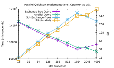
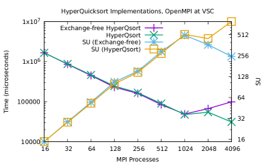
Figure 2: Strong scaling results, $n=10^{8}$ random doubles in the range $[0,10^{8}-1]$ on a medium-large InfiniBand cluster. Plotted running times and speed-up (SU) are the best observed over 43 measurements. Left plot shows parallel Quicksort versus exchange-free parallel Quicksort. Right plot shows HyperQuicksort versus exchange-free HyperQuicksort.

The plots in Figure 2 shows a few strong scaling results on a medium-sized InfiniBand cluster consisting of 2020 dual-socket nodes with two Intel Xeon E5-2650v2, 2.6 GHz, 8-core Ivy Bridge-EP processors and Intel QDR-80 dual-link high-speed InfiniBand fabric. The MPI library used is OpenMPI 3.0.0, and the programs were compiled with gcc 6.4 with optimization level -O3. The $n=10^{8}$ input elements are uniformly randomly generated doubles in the range from $[0,10^{8}-1]$, and $p$ varies from $2^{4}$ to $2^{12}$. The $p$ MPI processes are distributed with 16 processes per compute node. For each input, measurements were repeated 43 times with 5 non-timed, warm-up measurements, and the best observed times for the slowest processor are shown in the plots and used for computing speed-up. As can be seen, the exchange-free variant of parallel Quicksort gives consistently higher speed-up by about 20% than the corresponding standard variant with element exchanges up to about $1024$ processes. From then on, the number of elements per process of $n/p<100\,000$ becomes so small that the MPI_Allreduce on the vectors of pivots and the linear latency of the MPI_Alltoallv operation become more expensive than the explicit element exchanges. The exchange-free variant of HyperQuicksort is slightly faster than HyperQuicksort, but by a much smaller margin. Interestingly, with (almost) perfect pivot selection as in these experiments, standard parallel Quicksort seems preferable to Wagar’s HyperQuicksort.

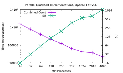
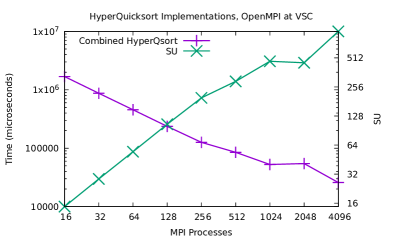
Figure 3: Strong scaling results, $n=10^{8}$ random doubles in the range $[0,10^{8}-1]$ on a medium-large InfiniBand cluster for the combined Quicksort implementation. Plotted running times and speed-up (SU) are the best observed over 43 measurements. Left plot shows combined, parallel Quicksort. Right plot shows combined HyperQuicksort.

To counter the degradation in the exchange-free variants for small $n/p$, the explicit exchange and exchange-free variants can be combined. Throughout the recursion in parallel Quicksort and HyperQuicksort, the number of elements per process $n^{\prime}$ stays the same (under the assumption that optimal pivots are chosen) whereas the number of processes is halved in each recursive call. Thus, the recursion is stopped when $n^{\prime}>cp/\log n$ for some chosen implementation and system dependent constant $c$, and the corresponding exchange-free variant invoked. By choosing $c$ well, this will give a smoother transition from parallel Quicksort for small per process input sizes to exchange-free Quicksort as $n/p$ grows. Results from these combined Quicksort variants are shown in Figure 3. With the constant $c$ chosen experimentally as $c=1500$, the combined Quicksort is never worse than neither standard nor exchange-free variant. Combined parallel Quicksort reaches a speed-up of more than 1000 on $p=4096$ processes. This speed-up, and the speed-up of 650 with $p=2048$ processes is larger than achieved with either parallel Quicksort and exchange-free Quicksort alone.

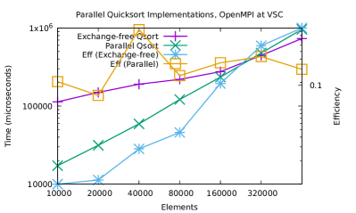
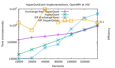
Figure 4: Weak scaling results on a medium-large InfiniBand cluster, $p=8192$, and number of elements per process varying from $n/p=10\,000$ to $n/p=640\,000$. The input elements are random doubles in the range $[0,10^{7}-1]$. Plotted running times and parallel efficiency are the best observed over 43 measurements. Left plot shows parallel Quicksort versus exchange-free parallel Quicksort. Right plot shows HyperQuicksort versus exchange-free HyperQuicksort.

The plots in Figure 4 show results from a weak scaling experiment where $p=8192$ is kept fixed, and the initial input size per process varies from $n/p=10\,000$ to $n/p=640\,000$ randomly generated doubles in the range $[0,10^{7}-1]$. The experimental setup is as for the strong scaling experiment. Beyond about $n/p=200\,000$ elements per process, the exchange-free variants perform better than the standard variants, reaching a parallel efficiency of $15\%$ for exchange-free Quicksort, and $12\%$ for exchange-free HyperQuicksort.

Repeating the experiments with random permutations and with integer type elements does not qualitatively change the results.

6 Concluding remarks

This note presented two new variants of parallel Quicksort for the classroom that trade explicit element exchanges throughout the Quicksort recursion against global selection of multiple pivots and a single element redistribution. All communication in the new variants is delegated to MPI collective operations, and the quality of the MPI library will co-determine the scalability of the implementations. For moderately large numbers of elements per process, these variants can be faster than standard parallel Quicksort variants by a significant factor, and can be combined with the standard, exchange-based variants to provide a smoothly scaling parallel Quicksort implementation.

Appendix A Standard parallel Quicksort algorithms

For completeness, this appendix gives pseudo-code for the two standard parallel Quicksort implementation variants, shown as Algorithm 3 (parallel Quicksort) and Algorithm 4 (HyperQuicksort). Algorithm 3 also shows how standard, parallel Quicksort can transition to exchange-free Quicksort when the input to be sorted raises above threshold relative to the number of processes employed. This is the combined Quicksort discussed in the main text. In order that all processes switch consistently, the maximum number of elements at any process is used as basis for the decisions. This can either be computed by a collective MPI_Allreduce operation, or an identical estimate for all processes can be used.

Algorithm 3 Standard parallel Quicksort of elements in $n$-element array $a$ for process $i\in\{0,\ldots,p-1\}$ and $p=2^{k}$.

1:procedure ParQsort($a,n,i\in\{0,\ldots,p-1\}$)

2:     if $p=1$ then

3:         return local-Qsort($a,n$)$\triangleright$ Sort locally

4:     else if $\max_{i\in\{0,\ldots,p-1\}}(n)>cp/(\log_{2}p+\log_{2}\max_{i\in\{0,\ldots,p-1\}}(n))$ then

5:         return ExchangeFreeQsort($a,n$)$\triangleright$ Sort locally

6:     else

7:         $x\leftarrow\mbox{{local-Choose}($a,n$)}$$\triangleright$ Local pivot selection

8:         $x^{\prime}\leftarrow\mbox{{global-Choose}($x$)}$$\triangleright$ Global consensus

9:         $n_{0}\leftarrow\mbox{{Partition}($a,n,x^{\prime}$)}$

10:         $\triangleright$ $a[0,n_{0}-1]\leq x^{\prime},a[n_{0},n-1]\geq x^{\prime}$

11:         if $i<p/2$ then

12:              Exchange($a+n_{0},n-n_{0},i+p/2,a^{\prime},n^{\prime}$)

13:              copy($a,n_{0},a^{\prime}+n^{\prime}$)

14:              $\triangleright$ Recursively sort new array $a^{\prime}$ in parallel

15:              return ParQsort($a^{\prime},n^{\prime}+n_{0},i\in\{0,\ldots,p/2-1\}$)

16:         else

17:              Exchange($a,n_{0},i-p/2,a^{\prime},n^{\prime}$)

18:              copy($a+n_{0},n-n_{0},a^{\prime}+n^{\prime}$)

19:              $\triangleright$ Recursively sort new array $a^{\prime}$ in parallel

20:              return ParQsort($a^{\prime},n^{\prime}+n-n_{0},i-p/2\in\{0,\ldots,p/2-1\}$)

21:         end if

22:     end if

23:end procedure

Algorithm 4 HyperQuicksort of elements in $n$-element array $a$ for process $i\in\{0,\ldots,p-1\}$ for $p=2^{k}$.

1:procedure HyperQsort($a,n,i\in\{0,\ldots,p-1\}$)

2:     local-Qsort($a,n$)$\triangleright$ Sort locally

3:     MergePartition(($a,n,i\in\{0,\ldots,p-1\}$))

4:end procedure

5:procedure MergePartition($a,n,i\in\{0,\ldots,p-1\}$)

6:     if $p=1$ then

7:         return $a$

8:     end if

9:     $x\leftarrow\mbox{{local-Choose}($a,n$)}$$\triangleright$ Local pivot selection $x=a[n/2]$

10:     $x^{\prime}\leftarrow\mbox{{global-Choose}($x$)}$$\triangleright$ Global consensus

11:     $n_{0}\leftarrow\mbox{{Split}($a,n,x^{\prime}$)}$$\triangleright$ $a[0,n_{0}-1]\leq x^{\prime},a[n_{0},n-1]\geq x^{\prime}$

12:     if $i<p/2$ then

13:         Exchange($a+n_{0},n-n_{0},i+p/2,a^{\prime},n^{\prime}$)

14:         Merge($a^{\prime},n^{\prime},a,n_{0},b$)

15:         return MergePartition($b,n^{\prime}+n_{0},i\in\{0,\ldots,p/2-1\}$)

16:     else

17:         Exchange($a,n_{0},i-p/2,a^{\prime},n^{\prime}$)

18:         Merge($a^{\prime},n^{\prime},a+n_{0},n-n_{0},b$)

19:         return MergePartition($b,n^{\prime}+n-n_{0},i-p/2\in\{0,\ldots,p/2-1\}$)

20:     end if

21:end procedure

References

- [1] M. Axtmann and P. Sanders. Robust massively parallel sorting. In Proceedings of the Ninteenth Workshop on Algorithm Engineering and Experiments (ALENEX), pages 83–97, 2017.
- [2] M. Axtmann, A. Wiebigke, and P. Sanders. Lightweight MPI communicators with applications to perfectly balanced quicksort. In 32nd IEEE International Parallel and Distributed Processing Symposium (IPDPS), 2018.
- [3] J. L. Bentley and M. D. McIlroy. Engineering a sort function. Software – Practice and Experience, 23(11):1249–1265, 1993.
- [4] A. Grama, G. Karypis, V. Kumar, and A. Gupta. Introduction to Parallel Computing. Addison-Wesley, second edition, 2003.
- [5] V. Harsh, L. V. Kalé, and E. Solomonik. Histogram sort with sampling. arXiv:1803.01237, 2018.
- [6] C. A. R. Hoare. Quicksort. The Computer Journal, 5(4):10–15, 1962.
- [7] J. JáJá. A perspective on quicksort. Computing in Science and Engineering, 2(1):43–49, 2000.
- [8] Y. Lan and M. A. Mohamed. Parallel quicksort in hypercubes. In Proceedings of the ACM/SIGAPP Symposium on Applied Computing (SAC): Technological Challenges of the 1990’s, pages 740–746, 1992.
- [9] MPI Forum. MPI: A Message-Passing Interface Standard. Version 3.1, June 4th 2015. www.mpi-forum.org.
- [10] M. J. Quinn. Analysis and benchmarking of two parallel sorting algorithms: Hyperquicksort and quickmerge. BIT, 29(2):239–250, 1989.
- [11] M. J. Quinn. Parallel Programming in C with MPI and OpenMP. McGraw-Hill, 2003.
- [12] P. Sanders, J. Speck, and J. L. Träff. Two-tree algorithms for full bandwidth broadcast, reduction and scan. Parallel Computing, 35(12):581–594, 2009.
- [13] R. Sedgewick and K. Wayne. Algorithms. Addison-Wesley, 4th edition, 2011.
- [14] C. Siebert and F. Wolf. Parallel sorting with minimal data. In Recent Advances in Message Passing Interface. 18th European MPI Users’ Group Meeting, volume 6960 of Lecture Notes in Computer Science, pages 170–177, 2011.
- [15] H. Sundar, D. Malhotra, and G. Biros. Hyksort: A new variant of hypercube quicksort on distributed memory architectures. In International Conference on Supercomputing (ICS), pages 293–302, 2013.
- [16] B. Wagar. Hyperquicksort – a fast sorting algorithm for hypercubes. In Hypercube Multiprocessors, pages 292–299. SIAM Press, 1987.