Theoretical X-ray light curves of young SNe II: the example of SN 2013ej

Abstract

The X-ray signal from hydrogen-rich supernovae (SNe II) in the first tens to hundreds of days after the shock breakout encodes important information about the circumstellar material (CSM) surrounding their progenitors before explosion. In this study, we describe a way to generate the SN II X-ray light curves from hydrodynamical simulations performed with the code Athena++, using the X-ray package XSPEC. In addition, we employ a radiation diffusion hydrodynamic code SNEC for generating the optical light curves in different bands. In this numerical setup, we model the X-ray and optical emission from a set of progenitor models, consisting of either two (red supergiant + low density steady wind), or three (red supergiant + dense CSM + low density steady wind) components. We vary the density in the wind and the slope in the CSM to see how these parameters influence the resulting X-ray and optical light curves. Among our models, we identify one that is able to roughly reproduce both optical and X-ray data of the well observed SN 2013ej. In order to achieve this, the slope of the dense CSM in this model should be steeper than the one of a steady wind ($\rho\propto r^{-2}$), and closer to $\rho\propto r^{-5}$. On the other hand, we show that too steep and extended CSM profiles may produce excessive X-ray emission in the first few tens of days, up to a few orders of magnitude larger than observed. We conclude that ability to reproduce the observed X-ray signal from SNe II together with their optical light curves is crucial in establishing the validity of different CSM models.

1. Introduction

Starting from their birth at zero-age main-sequence (ZAMS), isolated stars keep loosing mass through their lifetimes, largely in the form of steady radiation driven winds (see reviews of Kudritzki & Puls 2000; Puls et al. 2008; Smith 2014). It is convenient to estimate these winds in solar masses lost per year, $\dot{M}$, with the typical values ranging between $10^{-9}$ and $10^{-4}\,M_{\odot}\,{\rm yr}^{-1}$, depending on the observational diagnostics used to measure them (see Puls et al. 2006; Ramírez-Agudelo et al. 2017; Goldman et al. 2017 for measurements in the IR and radio, Bouret et al. 2005; Fullerton et al. 2006 in the UV, Cohen et al. 2010, 2011 in the X-rays). All modern stellar evolution codes take these mass losses into account using parameterized prescriptions for $\dot{M}$ as a function of stellar luminosity, temperature, and metallicity (commonly used are the ones of de Jager et al. 1988; Nieuwenhuijzen & de Jager 1990; Vink et al. 2001). For example, a $15\,M_{\odot}$ star at ZAMS becomes a red supergiant (RSG) with the mass slightly less that $13\,M_{\odot}$ by the end of its evolution (Sukhbold et al., 2016). Eventually, it undergoes core collapse and explodes, giving rise to a Type II supernova (SN II).

In this basic picture, the progenitor of a SN II consists of a RSG surrounded by the wind, the density of which reaches the values of at most $\sim$$10^{-14}\,{\rm g}\,{\rm cm}^{-3}$ next to the stellar surface and drops as $\rho\propto r^{-2}$ at larger distances. The influence of such wind on the optical SN light curve is negligible. For this reason, numerous hydrodynamical simulations aiming to reproduce the observed optical light curves of SNe II typically do not include this low density steady wind in the models (among many others, see the works of Bersten et al., 2011; Dessart et al., 2013; Utrobin & Chugai, 2017; Pumo et al., 2017). At the same time, even a very low density wind plays a crucial role in the production of X-ray signal from SNe II (Chevalier, 1982; Chevalier & Fransson, 2016).

Recently, due to the growing number of early observed, finely sampled SN II light curves (Anderson et al. 2014; Valenti et al. 2016; Förster et al. 2016; Hicken et al. 2017, see the online database by Guillochon et al. 2017), as well as more detailed comparisons to the numerical simulations (Nagy & Vinkó, 2016; Morozova et al., 2017b; Paxton et al., 2018; Moriya et al., 2018), we have come to realize that there may be a missing element in this picture. Agreement between the hydrodynamical models and observed light curves improves significantly with the addition of a dense compact circumstellar medium (CSM) in the mass range between $0.1$ and $0.8\,M_{\odot}$, surrounding the RSG before explosion. It appears to be surprisingly common, seen in as much as $\sim$$70\%$ of otherwise regular SNe II from the sample studied in Morozova et al. (2017b) (here, we are not considering SNe IIn, which are well known for their strong interaction with CSM, see Kiewe et al. 2012; Taddia et al. 2013). The formation mechanism of this CSM is far from being clear. It may be a result of wave-driven enhanced winds or outbursts in the last stages of stellar evolution (Quataert & Shiode, 2012; Shiode & Quataert, 2014; Fuller, 2017), form during the common envelope phase with a possible binary companion (Chevalier, 2012), and even have a disk-like shape (Andrews & Smith, 2017; McDowell et al., 2018). For many of these scenarios, it makes little sense to characterize the CSM by the value of $\dot{M}$, which implies a steady character of mass losses from the RSG.

Early observations of SNe II provide numerous hints that could help us measure the amount and probe the structure of this CSM. For instance, many of the early detected SNe II have narrow features in their spectra, which disappear within hours of observations (so called ‘flash spectroscopy’ Gal-Yam et al. 2014; Smith et al. 2015; Khazov et al. 2016; Yaron et al. 2017; Hosseinzadeh et al. 2018; Nakaoka et al. 2018; Bullivant et al. 2018). These observations are very important in constraining the properties of matter at the site of shock breakout, and above it. At the same time, numerical models of Morozova et al. (2017b), Paxton et al. (2018) and Moriya et al. (2018) suggest that the CSM needed to explain the early (first $\sim$30 days) photometry of SNe II is so dense, that the shock breakout itself happens within this CSM, close to its outer edge. Therefore, only the outer part of the CSM is flash ionized by the shock breakout light, while the most part of it cannot be probed by means of the flash spectroscopy. Another important observational constraint comes from the rapid rise of SNe II at the ultraviolet wavelengths (Gezari et al., 2015; Tanaka et al., 2016; Ganot et al., 2016).

In this study, we focus on the relatively early (first $\sim$$150$ days) X-ray signal from SNe II as a potential probe of the dense CSM surrounding the RSG before explosion. As of now, the early X-ray data on SNe II is still scarse, partly because of frequent non-detections, which can only place upper limits on the X-ray luminosity. Nevertheless, the sample of SNe of all types observed in X-rays has been steadily growing and currently consists of over 60 objects (Schlegel 2006; Immler 2007; Dwarkadas & Gruszko 2012, see the online database by Ross & Dwarkadas 2017). We have chosen SN 2013ej as an object of our investigation, because it has 6 X-ray data points in the first 150 days after explosion, as well as one of the best sampled photometric light curves among SNe II. We perform numerical simulations of the SN explosion and generate X-ray and optical light curves from a set of progenitor models, with and without dense CSM. Our study shows that it is possible to construct a model that includes dense CSM and provides a good fit for both optical and X-ray data of SN 2013ej. In previous literature, the influence of the enhanced mass loss in the last years of stellar evolution on its X-ray light curve was studied, for example, by Patnaude et al. (2015, 2017).

The paper is organized in the following way. We start from introducing SN 2013ej in Section 2. Section 3 outlines our numerical setup. Progenitor models that we use are described in Section 3.1. In this study, we work with three numerical codes, Athena++, XSPEC, and SNEC, which are described in Sections 3.2, 3.3, and 3.4, respectively. Section 4 shows the results obtained from models with regular low density RSG wind only. Section 5 shows the results obtained from models including dense CSM of a constant slope (one of the examples of which is a dense steady wind studied in Morozova et al. 2017a, 2018). Section 6 describes the results from models including dense CSM of a variable slope, similar to the accelerating wind studied in the works of Moriya et al. (2017, 2018). Section 7 is devoted to the conclusions.

2. Overview of SN 2013ej

The goal of our study is to present a way of generating SNe II X-ray light curves from hydrodynamical simulations, focusing on reproducing the data of SN 2013ej from a nearby well studied galaxy M74 (NGC 628). This SN was discovered very early, less than 1 day after the last non-detection, by the Lick Observatory Supernova Search (Dhungana et al., 2013; Kim et al., 2013; Shappee et al., 2013; Valenti et al., 2013; Lee et al., 2013), and has excellent photometric and spectroscopic coverage along the whole duration of its light curve (Valenti et al., 2014; Richmond, 2014; Bose et al., 2015; Huang et al., 2015; Yuan et al., 2016; Dhungana et al., 2016). Additional important information about SN 2013ej comes from the detection of its progenitor on the Hubble Space Telescope (HST) pre-explosion image (Fraser et al., 2014), search for a possible radio emission (Sokolovsky et al., 2013), which gave a negative result, and spectropolarimetric analysis of both the early (Leonard et al., 2013) and late (Kumar et al., 2016) epochs, which showed an unusually strong intrinsic polarization of the SN .

Semi-analytical studies and numerical simulations of SN 2013ej agree on the fact that it had an intermediate mass progenitor. Among the estimates on the ejected mass of this SN found in the literature are $12\,M_{\odot}$ (Bose et al. 2015, based on the semianalytical approach of Arnett 1980; Arnett & Fu 1989; Nagy et al. 2014), $\sim 10.6\,M_{\odot}$ (Huang et al. 2015, based on the hydrodynamical simulations), $13.8\pm 4.2\,M_{\odot}$ (Dhungana et al. 2016, based on the approach of Litvinova & Nadezhin 1983). Modeling the nebular emission lines, Yuan et al. (2016) found the ZAMS mass of the progenitor to be $12-15\,M_{\odot}$. Fraser et al. (2014) gives the range for the progenitor ZAMS mass $8-15.5\,M_{\odot}$, based on the analysis of its pre-explosion image. On the other hand, hydrodynamical simulations of Utrobin & Chugai (2017) suggest large ejecta mass of $23-26\,M_{\odot}$.

The classification type of SN 2013ej is somewhat transitional between IIP (plateau) and IIL (linear). After the fast initial rise it demonstrated a fast decline in magnitude (1.74 mag/100 days in $V$-band), and at the same time a relatively slow decline in the H$\alpha$ and H$\beta$ velocity profiles, which is typical for a linear subclass of SNe II (see Faran et al., 2014b, a; Bose et al., 2015). In Morozova et al. (2017a), we have shown that in order to reproduce this light curve behavior in numerical models, they must include some sort of dense circumstellar material (CSM) surrounding the RSG before the explosion (see also Das & Ray, 2017). The compactness (few thousands of solar radii) and the high density ($\sim 10^{-10}\,{\rm g}\,{\rm cm}^{-3}$) of the CSM, which provides the best fit to the data, suggests that this material could have been ejected from the RSG only a few years before the SN explosion. We have reanalyzed SN 2013ej as a part of a larger SN set in Morozova et al. (2017b), where we found that the best fitting model for its optical data has ZAMS mass $13\,M_{\odot}$, final energy $0.68\,{\rm B}$, and $0.49\,M_{\odot}$ of the CSM extending up to the radius $1800\,R_{\odot}$.

It should be mentioned that SN 2013ej indeed showed some signs of interaction between the ejecta and CSM, such as an unusually strong absorption feature in the blue wing of the H$\alpha$ P-Cygni trough (Chugai et al., 2007; Leonard et al., 2013) and presence of high-velocity components in H$\alpha$ and H$\beta$ profiles (Bose et al., 2015). At the same time, analysis of $\sim$$10$ images of SN 2013ej host galaxy in $\sim$$5$ years before the explosion suggests no significant variability in the progenitor, challenging the idea of eruptive outbursts in the last few years of stellar evolution, which could lead to the formation of CSM (Johnson et al., 2017).

The X-ray signal from SN 2013ej was first detected with Swift XRT (Margutti et al., 2013) and followed up with Chandra X-ray Observatory for five epochs (Chakraborti et al., 2016), until day 145 after the explosion. The X-ray data for this and other young SNe are available online in the Supernova X-ray Database (SNaX, Ross & Dwarkadas 2017). The details and analysis of the X-ray data are given in Chakraborti et al. (2016), where it was found that the observations are consistent with the steady mass loss rate $\dot{M}=2.6\times 10^{-6}\,M_{\odot}\,{\rm yr}^{-1}$ from a $M_{\rm ZAMS}=13.7\,M_{\odot}$ RSG over the last 400 years before its explosion. In this study we perform the analysis in the inverse direction compared to Chakraborti et al. (2016), starting from exploding the progenitor model with the wind attached to it, generating the X-ray signal from the output of the hydrodynamical simulation, and comparing it to the observational data. Based on the optical modeling suggesting the presence of high density CSM around the RSG, we attempt to incorporate the CSM in the X-ray models as well, to obtain a model that would fit well both optical and X-ray data.

3. Numerical Setup

To model X-ray and optical signal from SN 2013ej we use three open source numerical codes, Athena++ , XSPEC and SNEC , applied to the stellar evolution progenitor models from KEPLER (Sukhbold et al., 2016). In this section, we describe the progenitor models and numerical setup used in each code. Whenever possible, we base our choice of numerical parameters either on the optical light curve fit from Morozova et al. (2017b) or on the choice of parameters used in Chakraborti et al. (2016), in order to facilitate comparison with their work.

3.1. Pre-explosion models

The progenitor models used in this paper are non-rotating solar-metallicity red supergiants (RSGs) obtained with the stellar evolution code KEPLER (Weaver et al., 1978; Woosley & Heger, 2007, 2015; Sukhbold & Woosley, 2014; Sukhbold et al., 2016). We especially focus on the model with $M_{\rm ZAMS}=13\,M_{\odot}$, since this model provided the best fit to the optical data in Morozova et al. (2017b). At the onset of core collapse this model has mass $M_{\rm RSG}=11.56\,M_{\odot}$ and radius $R_{\rm RSG}=699\,R_{\odot}$. Unless explicitly indicated otherwise, all X-ray and optical light curves shown in this study are obtained from this model.

To generate the X-ray signal from a SN II it is essential to have a wind surrounding the RSG before its explosion. The X-ray emission originates in a thin shell between the two (forward and reverse) shock waves, which form after the original, radiation dominated post-explosion shock wave reaches the surface of the star (Chevalier & Fransson, 2016; Chakraborti et al., 2012). The X-ray luminosity is expected to depend on the mass loss rate of the wind $\dot{M}$, its velocity $v_{\rm wind}$ as well as the density slope in the wind and in the shocked stellar envelope (Chevalier & Fransson, 2003; Dwarkadas, 2014).

Observational estimates on the steady mass loss rates from the stars generally depend on the method used to measure them (Smith, 2014). The diagnostics based on measuring free-free emission in radio or IR (Wright & Barlow, 1975) are sensitive to the square of the wind density, $\rho^{2}$, and predict the mass loss rates in the range $10^{-7}-10^{-5}\,M_{\odot}\,{\rm yr}^{-1}$. Instead, the diagnostics based on measuring the strength of blueshifted P Cygni absorption features (Puls et al., 2008) depend linearly on density and predict the $\dot{M}$ values in the range $10^{-9}-10^{-6}\,M_{\odot}\,{\rm yr}^{-1}$ (see, for example Fullerton et al., 2006). It is expected that the methods measuring $\rho^{2}$ overestimate the mass loss rates due to the clumpy structure of the winds (Owocki & Puls, 1999; Bouret et al., 2005; Dessart & Owocki, 2005; Sundqvist & Owocki, 2013).

At the same time, growing observational evidence points on the enhanced mass loss during the last years of stellar evolution, probably in the form of eruptions (see, for example, Mauerhan et al., 2013; Ofek et al., 2014; Pastorello et al., 2008). In many cases, short signs of interaction with the CSM are seen in the early light curves of otherwise regular SNe II (Smith et al., 2015; Khazov et al., 2016; Yaron et al., 2017).

In the current study, we consider the following three kinds of the pre-explosion models:

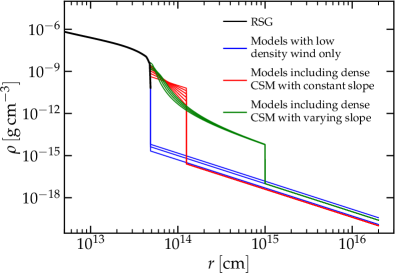
1) Models with low density wind only. We construct these models by attaching a steady wind with the density profile

$$\rho(r)=\frac{\dot{M}_{\rm low}}{4\pi r^{2}v_{\rm wind}}$$ (1)

to the surface of the RSG, and extending it all the way to the outer boundary of Athena++ computational domain ($2.0\times 10^{16}\,{\rm cm}$). For this kind of models, we take $v_{\rm wind}=10\,{\rm km}\,{\rm s}^{-1}$ and use the mass loss values from the range observed in steady state stellar winds, for example, $1-3\times 10^{-6}\,M_{\odot}\,{\rm yr}^{-1}$.

2) Models including dense CSM with constant slope. To construct these models we attach a high density CSM with the density profile

$$\rho(r)=\frac{\mathcal{K}}{r^{n}}\ ,$$ (2)

where $n$ and $\mathcal{K}$ are constant, to the surface of the RSG and extend it up to the radius $R_{\rm CSM}$. Slope $n=2$ corresponds to the case of a high density steady wind we considered in Morozova et al. (2017a, b). In this case, $\mathcal{K}=K\equiv\dot{M}_{\rm CSM}/(4\pi v_{\rm CSM})$, where $\dot{M}_{\rm CSM}$ is the effective mass loss and $v_{\rm CSM}$ is the velocity in CSM (in this work, we do not use $\dot{M}_{\rm CSM}$ anywhere else in the text). In Morozova et al. (2017b), we found that the best fitting model for SN 2013ej had $K=1.0\times 10^{18}\,{\rm g}\,{\rm cm}^{-1}$, $R_{\rm CSM}=1800\,R_{\odot}$, and the total CSM mass $M_{\rm CSM}=0.49\,M_{\odot}$. In this study, we vary the slope of the CSM, $n$, keeping its total mass and radial extent the same as in the best fitting model from Morozova et al. (2017b). For simplicity, we set $v_{\rm CSM}=10\,{\rm km}\,{\rm s}^{-1}$ everywhere in this CSM. Above the dense CSM, we attach the regular low density wind extending all the way to the outer boundary of the domain ($2.0\times 10^{16}\,{\rm cm}$).

3) Models including dense CSM with varying slope. Following Moriya et al. (2017), we construct this CSM as an accelerating wind in the form

$$\rho(r)=\frac{\dot{M}_{\rm acc}}{4\pi r^{2}v_{\rm acc}(r)}\ ,$$ (3)

with the velocity profile

$$v_{\rm acc}(r)=v_{0}+(v_{\infty}-v_{0})\left(1-\frac{R_{\rm RSG}}{r}\right)^{\beta}\ .$$ (4)

Here, $v_{0}$ is the wind velocity at the stellar surface and $v_{\infty}$ is the final wind velocity. We consider the models with $\beta=3.5$, $4.0$, $4.5$, and $5.0$, where the last value provided the best fit to the optical data of SN 2013fs, according to Moriya et al. (2017). Following their work, we fix $v_{\infty}$ to be $10\,{\rm km}\,{\rm s}^{-1}$, take $\dot{M}_{\rm acc}=10^{-3}\,M_{\odot}\,{\rm yr}^{-1}$ and place the outer boundary of the accelerating wind at $10^{15}\,{\rm cm}$. After that, we adjust the value of $v_{0}$ so that the total mass in this CSM is equal to $0.49\,M_{\odot}$, which we found in Morozova et al. (2017b) for SN 2013ej. We justify this step by the fact that the total mass of the accelerating wind derived in Moriya et al. (2017) for SN 2013fs is very close to the total mass of the steady wind derived in Morozova et al. (2017a) for the same SN. The resulting values of $v_{0}$ are of the order of $10\,{\rm m}\,{\rm s}^{-1}$. Above the accelerating wind, we attach the low density wind, which extends up to the outer boundary of the domain in Athena++ ($2.0\times 10^{16}\,{\rm cm}$).

The model of accelerating wind was proposed in Moriya et al. (2017) in order to achieve an agreement with the mass loss rate estimate of $10^{-3}\,M_{\odot}\,{\rm yr}^{-1}$ made by Yaron et al. (2017) for SN 2013fs. However, the estimate of Yaron et al. (2017) itself uses the assumption of a constant velocity steady wind. Therefore, we do not see a need to try reproducing its value by a model of accelerating wind. At the same time, a strength of this model is that the shock breaks out in the outer layers of the dense CSM (Moriya et al., 2018), flash ionizing a few percent of a solar mass of material in front of it. This would be enough to explain the narrow short-living spectral features seen in SNe II (Dessart et al., 2017; Boian & Groh, 2017).

To summarize, Figure 1 illustrates the density profiles of the three kinds of pre-explosion models considered in this study.

Figure 1.— Examples of the density profiles of the three kinds of models considered in this study. Black line shows the $M_{\rm ZAMS}=13\,M_{\odot}$ RSG, which is the same in all our models.

3.2. Athena++ setup

For this study, we use a pure hydro non-relativistic version of the relativistic magnetohydrodynamic code Athena++ (Gardiner & Stone, 2005, 2008; Stone et al., 2008). We assume spherical symmetry in our models and therefore use 1D version of the code.

Athena++ is an Eulerian code and the numerical grid is given in radial coordinates. We place our innermost grid zone at the radius, where the density of the pre-explosion model is equal to $10^{3}\,{\rm g}\,{\rm cm}^{-3}$ (radial coordinate $3.6\times 10^{9}\,{\rm cm}$ in our fiducial $13\,M_{\odot}$ model). This approximately corresponds to the excision of inner $2.4\,M_{\odot}$ of mass. This value is slightly higher than the remnant masses typically excised in this kind of simulations ($1.4-2\,M_{\odot}$), but we find that it significantly helps the numerical setup without compromising the results. The outermost grid zone is located at the radial coordinate $2.0\times 10^{16}\,{\rm cm}$. The grid consists of 10000 radial points spaced according to a geometric progression with the ratio between the neighboring cells equal to $1.0011$, so that the inner region is resolved finer than the outer one. This is necessary in order to resolve well the underlying RSG model. We note that even with the larger than usual excision mass the difference in density between the inner and the outer grid boundaries in our initial models is larger than 20 orders of magnitude. For the inner boundary we use a reflective boundary condition, and for the outer boundary we use an outflowing boundary condition.

We use adiabatic equation of state with the heat capacity ratio $\gamma=1.67$. In Athena++, as in SNEC (described below), we use a thermal bomb mechanism to explode the model. The explosion is initiated by injecting the internal energy into the innermost $20$ grid points over the time duration of $1\,{\rm s}$. Since Athena++ simulations do not account for self gravity, we omit the gravitational energy of the pre-explosion models when calculating the thermal bomb energy. Initial kinetic and internal energy of the models after the remnant excision is of the order of $0.03\,{\rm B}$, which is small compared to the typical final energies of SNe II ($0.5-1\,{\rm B}$). Therefore, in these simulations we take the thermal bomb energy equal to the final energy we want to reach, $E_{\rm fin}$. This allows us to put Athena++ simulations in correspondence with the SNEC simulations of the same final energy. The simulations are followed for 150 days after the explosion.

By default, Athena++ simulations presented here do not include radiation. However, in order to probe the influence of the radiative cooling on our results, we perform tests including a calibrated cooling function, as described below in Sections 4.3 and 6.

3.3. XSPEC setup

In order to generate the X-ray light curve, we analyze the output of Athena++ simulations using the X-ray package XSPEC (Arnaud, 1996).

We use the metallicity value $Z=0.295\,Z_{\odot}$, which was obtained in Chakraborti et al. (2016) based on the analysis of two-dimensional metallicity distribution of NGC 628 from Cedrés et al. (2012). The relative metal abundances are set according to Asplund et al. (2009). The resulting composition has mean atomic weight $\mu_{A}=1.24\,{\rm amu}$. Assuming complete ionization, this corresponds to the value of mean mass per particle $\mu=0.60\,{\rm amu}$ and the mean charge state averaged over all ions $q_{A}=\mu_{A}/\mu-1=1.07$. Using this value for $\mu$, we compute plasma temperature in each grid cell as $T=\mu P/\rho k_{\rm B}$, where $P$ is the pressure, $\rho$ is the density and $k_{\rm B}$ is the Boltzmann constant. The electron and ion number densities are computed as $n_{e}=q_{A}\rho/\mu_{A}$ and $n_{i}=\rho/\mu_{A}$, respectively.

In XSPEC, we use tbabs(apec) model in all grid points where it is applicable ($0.008<k_{B}T<64\,{\rm keV}$). The APEC model includes both line and continuum emission from a hot, optically thin plasma (Smith et al. 2001, see also http://atomdb.org). In the regions with higher temperatures ($64\leq k_{B}T<200\,{\rm keV}$) we use tbabs(bremss) model. The regions with temperatures higher than $200\,{\rm keV}$ are not expected to influence the observed part of the spectrum. Following Chakraborti et al. (2016), we adopt the value $d=9.57\pm 0.7\,{\rm Mpc}$ for the distance to the host galaxy of SN 2013ej, and the reshift value of $z=2.192\times 10^{-3}$ from NED.

The assumption of complete ionization for computing the ion and electron number densities in the shocked material is expected to work well in young supernova remnants, like the one considered in this study. Since the shock velocities at this stage are very high ($>500\,{\rm km}\,{\rm s}^{-1}$), the pre-shock matter is already largely ionized by the photons coming from the shock (Nymark et al., 2006; Fransson, 1984; Chevalier & Fransson, 1994). The recombination time in the shocked ejecta is generally longer than the cooling time (Nymark et al., 2006), leading to some highly ionized species being present at lower temperatures than they would be in the steady state case. Furthermore, as will be shown below, the relevant temperatures at these times stay very close to $\sim 10^{7}\,{\rm K}$, which roughly corresponds to the minimum of the radiative cooling function for the solar composition (Nymark et al. 2006, see also Eq. 6 below). Finally, since the value of metallicity we use for SN 2013ej is smaller than solar, even incomplete ionization of heavy metals would not change the electron and ion number densities with respect to the fully ionized ones in a significant way. However, we emphasize that this reasoning applies only in the early phase of a supernova remnant (first few hundreds of days), and in the case of older shocks it is important to solve for the non-equilibrium ionization state of the ejecta (see, for example, Borkowski et al., 1994, 2001; Dwarkadas et al., 2010).

Another important assumption that we use in our study is the equality between the ion and electron temperatures in the shocked ejecta. It is known that this assumption is not satisfied in the region behind the forward circumstellar shock, because the timescale for equipartition between the electrons and ions

$$t_{\rm eq}\approx 2.5\times 10^{7}\left(\frac{T_{e}}{10^{9}\,{\rm K}}\right)^{1.5}\left(\frac{n_{e}}{10^{7}\,{\rm cm}^{-3}}\right)^{-1}\,{\rm s}\ ,$$ (5)

where $T_{e}$ is the electron temperature, becomes too long due to the high temperature and low density of the plasma (Borkowski et al., 2001; Chevalier & Fransson, 2003, 2016). The reverse shock is expected to be in marginal equipartition. However, as will be seen from the results of the next section, the main part of the X-ray signal in our models comes from the dense and relatively cool shell between the forward and the reverse shock waves, where the temperatures of ions and electrons are expected to be equal.

To model the absorption of the X-ray signal with the multiplicative tbabs model, we compute the hydrogen column at each grid cell as $\int_{r}^{R_{\rm ext}}n_{H}dr$, where $r$ is the radial coordinate of the cell and $R_{\rm ext}$ is the outer boundary of the domain. When computing the hydrogen number density $n_{H}$, we use the hydrogen mass fraction of $X=0.748$. To the obtained value of hydrogen column we add the constant value for the external absorption column $n_{\rm ext}=4.8\times 10^{20}\,{\rm atoms}\,{\rm cm}^{-2}$. This value was used in Chakraborti et al. (2016), based on the Leiden Argentine Bonn (LAB) Survey of Galactic $H_{\rm I}$ (Kalberla et al., 2005).

Further in the text, by total X-ray flux we mean the flux calculated between $0.5$ and $8.0\,{\rm keV}$, while the soft and the hard fluxes correspond to the energy ranges $0.5-2.0\,{\rm keV}$ and $2.0-8.0\,{\rm keV}$, respectively.

3.4. SNEC setup

The optical ($V$-band) synthetic light curves shown in this study were obtained with SNEC (Morozova et al., 2015), a Lagrangian code that solves for the hydrodynamics and equilibrium-diffusion radiation transport in the expanding envelopes of core-collapse SNe, taking into account recombination effects and the presence of radioactive nickel.

As in Morozova et al. (2017b), we excise the inner part of the RSG models at the mass coordinate of silicon/oxygen interface in their composition profiles, because it approximately corresponds to the point of shock revival in the core-collapse explosion mechanism simulations (e.g., Müller et al., 2012; Summa et al., 2016; Suwa et al., 2016; Burrows et al., 2016; Radice et al., 2017). For a $13\,M_{\odot}$ model this interface is located at the mass coordinate $\approx 1.6\,M_{\odot}$. We assume that all matter deeper than that collapses to form a neutron star. After the remnant is excised, we initiate the explosion by injecting the internal energy $E_{\rm bomb}=E_{\rm fin}-E_{\rm init}$, where $E_{\rm fin}$ is the desired final energy and $E_{\rm init}$ is the total initial (negative, mostly gravitational) energy, into the inner $0.02\,M_{\odot}$ of the model for a duration of $1\,{\rm s}$.

SNEC uses the equation of state by Paczyński (1983). The ionization fractions of hydrogen and helium needed for the equation of state are found following the approach of Zaghloul et al. (2000). The numerical grid consists of 1000 mass cells, with the finer resolution in the interior, where the explosion is initiated, and especially fine resolution towards the outer boundary, in order to resolve the photosphere at early times (Morozova et al., 2015, 2016, 2017a). In SNEC simulations we omit the low density wind, because it introduces unnecessary numerical challenge in the form of a very small timestep. From the previous works (see, for example, Moriya et al., 2011) we know that the wind with mass loss rates $<10^{-5}\,M_{\odot}\,{\rm yr}^{-1}$ has a negligible effect on the optical light curve. Therefore, the outer boundary of SNEC grid coincides either with the RSG surface, or with the external radius of the high density wind, if it is included in the model.

The Rosseland mean opacity is computed from OPAL Type II opacity tables (Iglesias & Rogers, 1996) at high temperatures ($T>10^{4.5}\,{\rm K}$) and from the tables of Ferguson et al. (2005) at low temperatures ($10^{2.7}<T<10^{4.5}$). In SNEC we use the opacity floor, which is meant to account for the line broadening in the rapidly expanding stellar envelope as well as possible non-thermal ionization and excitation by gamma-rays, the effects that are not included in the opacity tables (see, for example, Blinnikov, 1996; Bersten et al., 2011). The value of the opacity floor in our simulations is computed from the compositional profile and equal to $0.01\,{\rm cm}^{2}\,{\rm g}^{-1}$ for the regions with solar metallicity $Z=0.02$, $0.24\,{\rm cm}^{2}\,{\rm g}^{-1}$ for $Z=1$, with the linear dependence in between. Before the explosion we smoothen the composition profiles by passing a “boxcar” with a width of $0.4\,M_{\odot}$ through the models four times. The amount of radioactive ⁵⁶Ni in SN 2013ej is taken to be $0.0207\,M_{\odot}$ (Valenti et al., 2016).

Photometric light curves are computed assuming black body emission and using the MATLAB package for astronomy and astrophysics for calculating specific wave bands (Ofek, 2014). In SNEC, the radiation temperature is assumed to be equal to the effective temperature $T_{\rm eff}=\left(L/4\pi\sigma_{\rm SB}R_{\rm ph}^{2}\right)^{1/4}$, where $L$ is the bolometric luminosity, $\sigma_{\rm SB}$ is the Stefan-Boltzmann constant and $R_{\rm ph}$ is the photospheric radius corresponding to the optical depth $\tau=2/3$. One of the caveats of this approach is that it assumes the equality between the temperatures of matter and radiation at the photosphere location, which may not be true for some models, including explosions of RSGs. In reality, the opacity in the regions below the photosphere is dominated by scattering, while the radiation color is determined by deeper layers, where the absorption opacity is still large enough (so called, ‘color shell’, Nakar & Sari 2010). For this reason, the photometric light curves returned by SNEC generally rise faster than the light curves obtained from more sophisticated multi-group radiation-hydrodynamics codes (for example, STELLA, Paxton et al. 2018). If anything, this means that it is even more challenging for those codes to reproduce the fast rising light curves of SNe II with bare RSG models without CSM. For this reason, the amount of CSM needed to explain the observed light curves with those codes is comparable, and in some cases larger than the one we need in SNEC (see, for example, Moriya et al., 2017; Paxton et al., 2018).

4. Results from the models with low density wind only

In this Section we focus on the models consisting of a pre-explosion RSG and a low density wind only. Most of the previous analytical and numerical studies of the X-ray emission from SNe II were devoted to this class of models (see, for example, Chevalier & Fransson, 1994, 2003, 2016; Nymark et al., 2006).

4.1. Hydrodynamical evolution of the models and their X-ray signal

Figure 2 describes the hydrodynamical evolution of $13\,M_{\odot}$ RSG model with a $\dot{M}=2\times 10^{-6}\,M_{\odot}\,{\rm yr}^{-1}$ wind. After the initial post-explosion shock wave reaches the surface of the RSG, it gives rise to a forward shock wave propagating into the low density wind and to a reverse shock wave propagating backwards into the shocked ejecta. The top panel of Figure 2 shows the temperature profile of the two shock waves, and the middle panel shows their density. The bottom panel of Figure 2 shows the total X-ray flux from each numerical grid cell after taking into account the absorption by all material above that cell, i. e., as seen by a remote observer.

Figure 2.— Evolution of the temperature profile (top panel), the density profile (middle panel), and the X-ray emission from each grid cell (bottom panel) of the forward and reverse shock waves in $13\,M_{\odot}$ RSG model with $\dot{M}=2\times 10^{-6}\,M_{\odot}\,{\rm yr}^{-1}$ wind. This plot shows that the most part of X-ray emission comes from the dense part of ejecta between the forward and reverse shock waves. The hot forward shock wave makes marginal contribution to the signal, justifying our assumption of equipartition between ions and electrons. At the same time, the X-ray emission coming from the front of the reverse shock wave is largely absorbed by the dense intermediate part of the shocked ejecta.

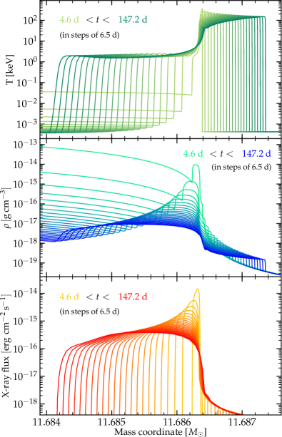
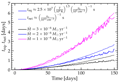
Figure 2 shows that the majority of the X-ray flux is coming from the shocked ejecta at the interface between the forward and the reverse shock waves. The forward shock wave itself generally has too high temperatures and too low densities to produce detectable X-ray signal, while the radiation from the front of the reverse shock wave is largely absorbed by the external layers. It is clear from Figure 2 that the maxima of X-ray radiation closely follow the regions of maximum density, which justifies the assumption of equality between the electron and ion temperatures used in our analysis. While it is known that due to the slow Coulomb equipartition the electron temperature immediately behind the reverse and especially the forward shock wave may be much smaller than the ion temperature, the dense interface region between the shocks is expected to be in equipartition at early times (see, for example, Fig.1 of Chevalier & Fransson, 2016). To better illustrate this, in Figure 3 we plot the equipartition timescale, $t_{\rm eq}$, given by Eq. 5, as well as the timescale $t_{\rm nei}$, which is needed to achieve equilibrium ionization (Dwarkadas et al., 2010). Both timescales shown in Figure 3 are calculated at the point of maximum of X-ray flux in our models. By day $\sim 150$ they are still small with respect to the light curve time.

Figure 3.— The equipartition timescale between ions and electrons, $t_{\rm eq}$, as well as the timescale $t_{\rm nei}$, which is needed to achieve equilibrium ionization, calculated at the point of maximum X-ray flux in our models.

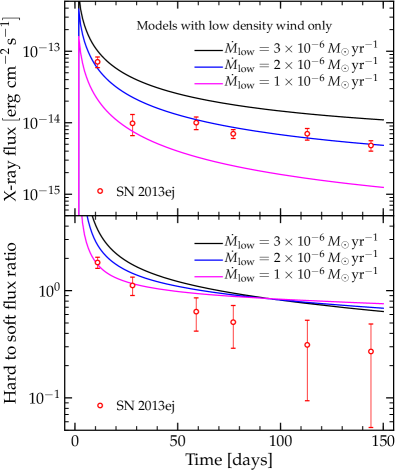
In Figure 4 we show the sum of the X-ray contributions from all individual numerical cells after taking into account the external absorption for each cell. The top panel of Figure 4 shows the total X-ray flux we obtain from the models with low density wind only having the mass loss rates of $1\times 10^{-6}$, $2\times 10^{-6}$ and $3\times 10^{-6}\,M_{\odot}\,{\rm yr}^{-1}$. The model with $\dot{M}=2\times 10^{-6}\,M_{\odot}\,{\rm yr}^{-1}$ reproduces well the observed total flux from SN 2013ej. This agrees with the result of Chakraborti et al. (2016), where the mass loss rate from SN 2013ej was estimated as $\dot{M}=(2.6\pm 0.2)\times 10^{-6}\,M_{\odot}\,{\rm yr}^{-1}$, based on the XSPEC fit of the X-ray spectra.

At the same time, the bottom panel of Figure 4 shows that our model with $\dot{M}=2\times 10^{-6}\,M_{\odot}\,{\rm yr}^{-1}$ cannot reproduce correctly the ratio between the soft and the hard components of the X-ray signal. In the observed data, the soft component starts to dominate already after day $\sim 30$, and by day $\sim 150$ it is about 4 times more energetic than the hard component. On the other hand, in our model the ratio between the soft and hard X-ray components by the end of simulation is only $\sim 1.5$.

Figure 4.— Top panel: Total X-ray flux obtained from $13\,M_{\odot}$ RSG model with the low density wind of different mass loss rates $\dot{M}$, compared to the observational data of SN 2013ej. Bottom panel: The ratio between hard ($2.0-8.0\,{\rm keV}$) and soft ($0.5-2.0\,{\rm keV}$) components of the obtained X-ray signal, compared to the values observed in SN 2013ej.

4.2. Dependence on the progenitor ZAMS mass and final energy

Figure 5.— Top panel: Total X-ray flux from the models with different progenitor ZAMS mass and final energy compared to the fiducial model. Bottom panel: Total, soft and hard X-ray flux for the model with $M_{\rm ZAMS}=13\,M_{\odot}$ and $E_{\rm fin}=0.4\,{\rm B}$, which demonstrates the best agreement with the X-ray data among the models with low density wind only.

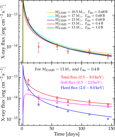
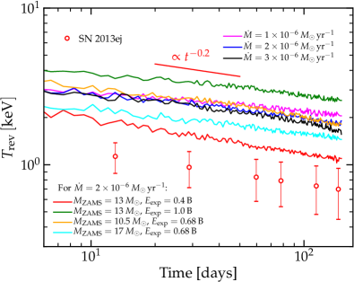
To check the dependence of this result on the model parameters, we performed the simulations for different progenitor ZAMS masses ($10.5$ and $17\,M_{\odot}$) and explosion energies ($0.4$ and $1.0\,{\rm B}$) using mass loss rate $\dot{M}=2\times 10^{-6}\,M_{\odot}\,{\rm yr}^{-1}$. The top panel of Figure 5 shows the total X-ray flux from these models. As expected from the analytical works (see, for example, Chevalier & Fransson, 2016), the total flux is mostly determined by the mass loss rate of the wind and depends weakly on the explosion energy. Instead, the shock temperature, which is proportional to the second degree of ejecta velocity (Chevalier & Fransson, 2016), depends almost linearly on the explosion energy. Therefore, the model with the explosion energy $0.4\,{\rm B}$, shown in the bottom panel of Figure 5, demonstrates much better agreement with the observed ratio between the soft and hard components of X-ray flux. Figure 6 shows the ejecta temperature at the maximum of the X-ray flux for all our models with low density wind. For comparison, with red markers we show the reverse shock temperature estimated in Chakraborti et al. (2016) from fitting the X-ray spectra with XSPEC.

Figure 6.— Comparison of the ejecta temperature at the maximum of X-ray flux in our models to the reverse shock temperature derived from fitting the observed X-ray spectra in Chakraborti et al. (2016). The model with $M_{\rm ZAMS}=13\,M_{\odot}$ and $E_{\rm fin}=0.4\,{\rm B}$ shows the best agreement with the observed hard to soft flux ratio, even though its ejecta temperature is slightly higher than the reverse shock temperature from Chakraborti et al. (2016). All the models demonstrate correct $\propto t^{-0.2}$ behavior.

Figure 7.— Top panel: Color coded ratio of $\chi^{2}$ to $\chi^{2}_{\rm min}$ at each point of the $M_{\rm ZAMS}-E_{\rm fin}$ grid of models without CSM for SN 2013ej. The black square indicates the best fitting model to the optical data between day 38 ($\approx$ slope break in the quasibolometric light curve of this SN) and day 99 (end of plateau). Bottom panel: $V$-band light curves obtained with SNEC compared to the observational data. The best fitting model is shown in black, while the colored lines show the light curves from the models marked by crosses of the corresponding color in the top panel.

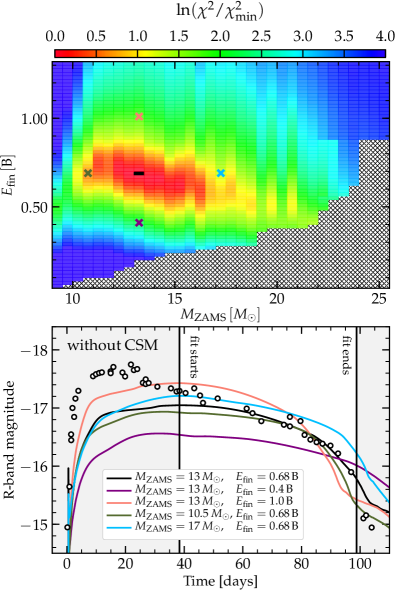
At the same time, from the numerical modeling of SN 2013ej optical light curve performed in Morozova et al. (2017b), we know that the models with progenitor ZAMS masses $10.5$ and $17\,M_{\odot}$ and explosion energies $0.4$ and $1.0\,{\rm B}$, shown in Figure 5, are not consistent with the optical data as well as our fiducial model. To illustrate this, Figure 7 shows the results obtained in Morozova et al. (2017b) for SN 2013ej without CSM. We reiterate that none of our models without a CSM was able to reproduce the early rise and subsequent decline seen in all (including red) bands of the optical data. Therefore, the models without CSM were compared to the data only starting from the approximate moment of the slope break in quasibolometric light curve, when the impact of the CSM is thought to become small. This moment is marked in Figure 7 as the start of the fit, while the end of the fit coincides with the transition from the plateau to the radioactive ⁵⁶Ni tail, when the radiation diffusion approach of SNEC is no longer valid.

The top panel of Figure 7 shows the distribution of $\chi^{2}$ for the grid of models in $M_{\rm ZAMS}-E_{\rm fin}$ parameter space from Morozova et al. (2017b), without CSM. Color coded is the natural logarithm of the ratio $\chi^{2}/\chi^{2}_{\rm min}$, where $\chi^{2}_{\rm min}$ corresponds to the best fitting model. The black rectangle shows the position of the best fitting model with $M_{\rm ZAMS}=13\,M_{\odot}$ and $E_{\rm fin}=0.68\,{\rm B}$, and the $V$-band light curve of this model is shown in the bottom panel with black solid line. The crosses in the top panel mark the position of the additional models, whose X-ray signals are plotted in the top panel of Figure 5. The light curves of these models are shown in the bottom panel with the corresponding colors. While the $10.5\,M_{\odot}$ light curve is rather close to the best fit model, the other three clearly do poorer job in representing the obesrvational data.

4.3. The effect of radiative cooling

To investigate the effect of radiative cooling in our models due to the X-ray emission, we performed a test simulation, where it was taken into account. We use the cooling function in the form

$$\Lambda=AT_{6}^{-\alpha}+BT_{6}^{\beta}\ ,$$ (6)

where $T_{6}=T/10^{6}\,{\rm K}$ (Chevalier & Fransson, 2016). This function was calibrated in Nymark et al. (2006) based on the hydrodynamical simulations of the radiative shocks, including time-dependent ionization balance and multilevel ion calculations. We use the solar composition values of the parameters $A$, $B$, $\alpha$ and $\beta$ from Table 2 of Nymark et al. (2006), namely, $A=8.0\times 10^{-23}\,{\rm erg}\,{\rm cm}^{3}\,{\rm s}^{-1}$, $B=2.3\times 10^{-24}\,{\rm erg}\,{\rm cm}^{3}\,{\rm s}^{-1}$, $\alpha=0.9$ and $\beta=0.5$. We apply the cooling function at each time step after the initial shock wave hits the boundary between the underlying RSG and the wind, by adding the term $-\Lambda n_{e}n_{i}dt$ to the energy density in the region between the forward and reverse shock waves, assuming complete ionization in this region. The position of the forward shock is found from the temperature maximum, while the position of the reverse shock coincides with the maximum of the radial velocity.

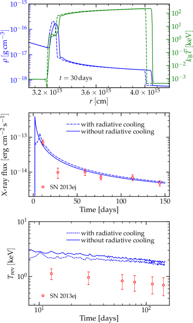
Figure 8 summarizes the result of this test. We find that the radiative cooling indeed leads to a slightly higher density in the shell between the forward and reverse shocks, as well as to a slightly lower temperature in that region. However, this effect is weak in our models, and does not lead to a better agreement with the observed X-ray data. Note that we use the cooling function calibrated for the solar composition, while the metallicity at the explosion cite of SN 2013ej is significantly subsolar (Chakraborti et al., 2016). If anything, we expect that at lower metallicities the X-ray radiative cooling would be weaker. In fact, at the temperatures of interest $\lesssim 2.24\,{\rm keV}$ ($2.6\times 10^{7}\,{\rm K}$) the X-ray emission (and cooling) is dominated by the line emission from metals (Chevalier & Fransson, 2016). Indeed, the metal rich compositions studied in Nymark et al. (2006) resulted in much higher values of the coefficients of Equation (6). We emphasize that in order to obtain the X-ray signal with XSPEC we used the observed subsolar value of the metallicity, $Z=0.295\,Z_{\odot}$.

To conclude this section, among the models including low density wind only we could not find the one that would give a simultaneous fit to the X-ray signal, including its total flux and ratio between the soft and hard components, as well as to the optical data.

Figure 8.— Top panel: Temperature and density in the shocked ejecta of $13\,M_{\odot}$ model with $\dot{M}=2\times 10^{-6}\,M_{\odot}\,{\rm yr}^{-1}$ at $t=30\,{\rm days}$. Solid lines represent the fiducial model, and dashed lines represent the model taking into account radiative cooling as described in the text. Middle panel: Total X-ray flux from the models with and without radiative cooling. Bottom panel: Ejecta temperatures at the maximum of X-ray flux for the models with and without radiative cooling.

5. Results from the models including dense CSM with constant slope

In this section, we describe the optical and X-ray light curves from the models consisting of a RSG, a dense CSM with the constant slope $n$, and a low density wind.

The most commonly studied case of such CSM is the one with $n=2$, because it has clear physical interpretation as a constant velocity steady wind. In Morozova et al. (2017a), we focused on this sort of CSM in order to explain the early photometry of three SNe II with various decline rates of the light curve, from almost flat Type IIP (plateau) SN 2013fs to the rapidly declining Type IIL (linear) SN 2013by, where SN 2013ej represented the object of somewhat transitional type between the two. In the subsequent work, Morozova et al. (2017b), we generalized this approach by fitting the optical light curves of 20 well observed SNe II and deducing their model parameters, again including SN 2013ej in the set. According to our findings, the best fitting model for SN 2013ej had $0.49\,M_{\odot}$ (here, we round up this value to $0.5\,M_{\odot}$) of the dense $n=2$ CSM extending up to the radial coordinate $R_{\rm CSM}=1800\,R_{\odot}$. Therefore, our first goal was to check whether the same progenitor model can reproduce the X-ray light curve of SN 2013ej, after we supplement it with a low density regular RSG wind.

Figure 9.— Top panel: Total ($0.5-8.0\,{\rm keV}$) X-ray flux from the model consisting of an $M_{\rm ZAMS}=13\,M_{\odot}$ RSG, the high density steady wind with a total mass of $0.5\,M_{\odot}$, and the low density wind with different values of mass loss $\dot{M}_{\rm low}$. The final energy of the model is $0.68\,{\rm B}$ in all cases. Bottom panel: The ratio between hard ($2.0-8.0\,{\rm keV}$) and soft ($0.5-2.0\,{\rm keV}$) components of the obtained X-ray signal, compared to the values observed in SN 2013ej.

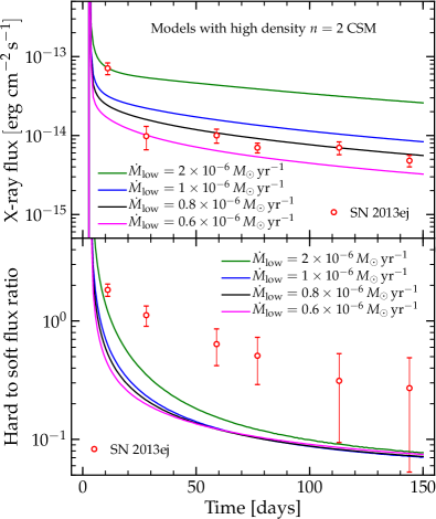
Figure 9 shows the X-ray light curves obtained from this model for different values of the mass loss in the low density wind. The final energy of the model is $0.68\,{\rm B}$ in all cases (Morozova et al., 2017b). From the top panel of Figure 9, one can see that the model with $\dot{M}_{\rm low}=2\times 10^{-6}\,M_{\odot}\,{\rm yr}^{-1}$ agrees well with the total observed X-ray flux of SN 2013ej. However, the bottom panel of this figure shows that for all values of $\dot{M}_{\rm low}$ the simulated X-ray emission is too soft compared to the observed one.

Figure 10.— Density profiles of the models including dense CSM with different slopes $n$.

In this model, as well as all other models of this section, the majority of the X-ray flux is coming from the shocked ejecta between the forward and reverse shock waves formed at the interface between the high density CSM and the low density wind (think of Figure 2 at the outer edge of dense CSM instead of the RSG surface). The softness of the synthetic X-ray light curve seen in the bottom panel of Figure 9 tells us that the temperature of the reverse shock wave is too low. One way to increase the shock temperature without changing the final energy of the model is to increase the slope of the CSM. In a steeper CSM, the original post-explosion shock wave can accelerate to larger velocites and, consequently, heat up the material to higher temperatures. Indeed, analytical results of Chevalier & Fransson (2016) suggest that the temperature in the reverse shock is proportional to the squared velocity of ejecta (although, the slope exponent $n$ itself enters the equation for the temperature as $(n-2)^{-2}$).

Figure 11.— Top panel: Total ($0.5-8.0\,{\rm keV}$) X-ray flux from the models shown in Figure 10. The final energy of the models is $0.68\,{\rm B}$ in all cases. Bottom panel: The ratio between hard ($2.0-8.0\,{\rm keV}$) and soft ($0.5-2.0\,{\rm keV}$) components of the obtained X-ray signal, compared to the values observed in SN 2013ej.

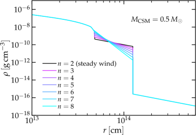
This motivates us to consider the CSM of different slopes from $n=2$ to $n=8$ with the density profiles shown in Figure 10 (the black curve in this plot corresponds to the steady wind used in Figure 9). In Morozova et al. (2017b), we demonstrated that the confidence regions around the best fitting models in the parameter space of the dense CSM were aligned with the isocontours of its total mass. This led us to a conclusion that the total mass of the CSM is better constrained by our models than its density and extent taken separately. Therefore, when constructing the models of dense CSM in Figure 10, we imposed the condition of constant total CSM mass, $M_{\rm CSM}=0.5\,M_{\odot}$, as derived in Morozova et al. (2017b) for SN 2013ej. In addition, we fixed the external radius of the CSM to $1800\,R_{\odot}$. This agrees with the compactness of the dense CSM found in observations (see, for example, Yaron et al., 2017).

Figure 12.— Top panel: $R$-band optical light curves obtained from the models shown in Figure 10. For comparison, black dashed line shows the light curve from a bare RSG without the dense CSM. The gray shaded area marks the region after the end of plateau, where the radiation diffusion approach used in SNEC is not valid. The total CSM mass of $0.5\,M_{\odot}$ is common between the models with different slope $n$. Bottom panel: Photospheric velocities of the same models versus the line velocities measured from the spectra of SN 2013ej in Dhungana et al. (2016) and Utrobin & Chugai (2017).

Figure 13.— The model from our set, which demonstrates agreement with both optical (top panel) and X-ray (bottom panel) data of SN 2013ej. The parameters of this model are: $M_{\rm ZAMS}=13\,M_{\odot}$, $E_{\rm fin}=0.68\,{\rm B}$, $M_{\rm CSM}=0.5\,M_{\odot}$, $R_{\rm ext}=1800\,R_{\odot}$, $n=5$, $\dot{M}_{\rm low}=0.9\times 10^{-6}\,M_{\odot}\,{\rm yr}^{-1}$.

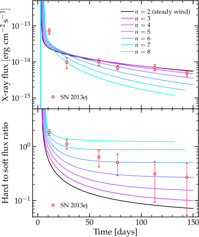
In Figure 11, we plot the total X-ray flux (top panel) and the ratio between the hard and soft components of this flux (bottom panel) from the models shown in Figure 10. It confirms our expectation that the X-ray signal becomes harder with the increasing slope of the CSM. The total X-ray flux changes as well, but to a smaller extent.

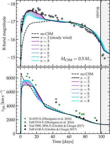
In the top panel of Figure 12, we plot the optical ($R$-band) light curves obtained from the same models using SNEC. Black markers show the data observed from SN 2013ej. Gray shaded region marks the end of plateau, after which the assumptions used in SNEC are no longer valid. For comparison, the model without the dense CSM is shown by the black dashed line (the same as black solid line in the bottom panel of Figure 7). Figure 12 shows that the CSM profiles with $n$ between 2 and $\sim$5 produce very similar light curves. The light curves start to deviate significantly only for the steep CSM profiles with $n>5$. However, taking into account that the difference in density between the $n=2$ and $n=8$ CSM profiles reaches few orders of magnitude (see Figure 10), we find that the maximum variation of $\sim$$0.4\,{\rm mag}$ between their light curves is rather small. This supports our assumption that the total CSM mass is one of the main parameters constrained by the hydrodynamical models of optical light curves.

The bottom panel of Figure 12 shows the velocity at the photosphere location, $v_{\rm ph}$, of the models from Figure 10. In the literature, the photospheric velocity is commonly compared to the velocities of Si or Fe lines measured from the SN spectra. In the bottom panel of Figure 12, the green markers indicate the velocities of Si $6355\,$Å and FeII $5318\,$Å lines found from the spectra of SN 2013ej in Dhungana et al. (2016). There are many more lines analyzed in the work of Dhungana et al. (2016), and the velocities of different lines measured from the same spectra show very large scatter, differing by $2000-4000\,{\rm km}\,{\rm s}^{-1}$ and more (see their Figure 20), but the Si $6355\,$Å and FeII $5318\,$Å lines correspond to the lowest velocities found at the early and late times, respectively. In addition, the black markers in the bottom panel of Figure 12 indicate the velocities of NaI $5890$, $5896\,$Å doublet and FeII $6148\,$Å line found from the same spectra by Utrobin & Chugai (2017). The largest disagreement between the measured line velocities and the photospheric velocity of our models is seen on day 44. In general, the qualitative agreement between the photospheric and line velocities that we find in Figure 12 is similar to the one seen in the models of Utrobin & Chugai (2017), which may be surprising given the large difference between the best fitting model parameters derived for SN 2013ej in Morozova et al. (2017b) and Utrobin & Chugai (2017).

However, we would like to emphasize that it is not at all obvious that the photospheric velocity of the numerical models should coincide with the Fe or Si line velocities measured from the spectra. Instead, the recent work of Paxton et al. (2018) demonstrated that the material velocity at the location where the Sobolev optical depth of the FeII $5169\,$Å line, $\tau_{\rm Sob}$, is equal to $1$ provides a much better match to the observations than the photospheric velocity. They find that the velocities found at $\tau_{\rm Sob}=1$ and $\tau=2/3$ start to disagree substantially after day $\sim$30 and may differ by up to a $1000\,{\rm km}\,{\rm s}^{-1}$ and more. Currently, we do not have the capability to estimate the $\tau_{\rm Sob}=1$ velocity of the FeII $5169\,$Å line from the hydrodynamical output of SNEC, but we plan to work on it in the future.

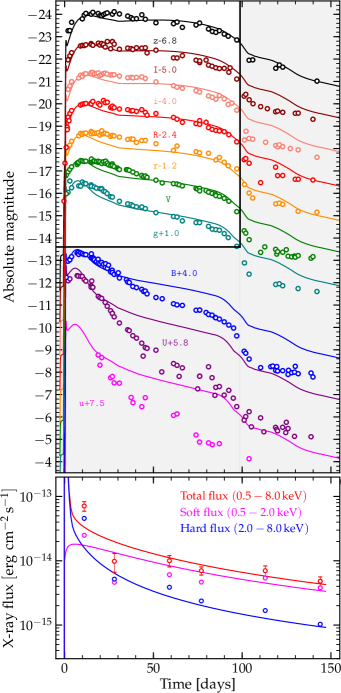
Finally, Figure 13 represents the main result of this section by showing a candidate model that can reproduce both optical and X-ray data of SN 2013ej. Here, we summarize the parameters of this model. It is based on the $13\,M_{\odot}$ (at ZAMS) RSG having final energy of $0.68\,{\rm B}$, which is necessary to reproduce the plateau part of the observed optical data. It has $0.5\,M_{\odot}$ of the dense compact ($R_{\rm CSM}=1800\,R_{\odot}$) CSM, the presence of which is suggested by the rapidly rising early optical data. The density in the CSM drops as $\rho\propto r^{-5}$, which ensures that its outermost region is sufficiently accelerated in order to reproduce the ratio between the hard and soft components of the observed X-ray emission. Above the dense CSM, this model has regular low density RSG wind with mass losses of $\dot{M}_{\rm low}=0.9\times 10^{-6}\,M_{\odot}\,{\rm yr}^{-1}$ needed to reproduce the total X-ray flux from SN 2013ej.

Since our numerical simulations involve many approximations in both optical and X-ray components (see Sections 3.2-3.4), the model shown in Figure 13 cannot be taken as a final word on the progenitor of SN 2013ej. Moreover, in this study we did not attempt to minimize the residuals and find an optimal fit across a grid of all parameters used in our models. Nevertheless, there are few general conclusions that can be drawn from this section. First of all, it shows that inclusion of a dense CSM does not make the model incompatible with the observed X-ray emission. In other words, the qualitative agreement with the early X-ray signal seen in the bottom panel of Figure 13 is as good as the one from Figure 5. The main difference between these two scenarios is in the location of the reverse shock wave, which produces the bulk of the X-ray emission. In the models with low density wind only, this reverse shock wave probes the surface region of the RSG, while in the models with the dense CSM, it probes the outermost layer of the CSM.

Second, this result shows that the early X-ray signal may be used as an important complementary piece of information in constraining the properties of the dense CSM surrounding RSGs before explosion. Analysis of this section shows that the CSM with constant $n=2$ slope along its entire extension produces the reverse shock wave that is too cold to fit the observed X-ray emission in the first few tens to hundreds of days. In reality, it is likely that the radiative cooling during and after the shock breakout will make the temperature of the shock wave even lower, and the X-ray emission even softer for the same CSM configuration. Therefore, we conclude that the density profile should be steeper than $n=2$ at least in some regions of the dense CSM, if not along its entire extension, to ensure the efficient acceleration of its outermost layer. Generally, this conclusion is in agreement with the idea of accelerating wind, proposed in the works of Moriya et al. (2017, 2018). At the same time, for now we refrain from explaining the origin of the dense CSM by either accelerating or steady wind, because our models are not sensitive to the pre-explosion velocities in the CSM (as long as they are much smaller than the post-explosion velocities of a few tens of thousands of ${\rm km}\,{\rm s}^{-1}$) and, therefore, cannot constrain its formation history. We consider the models even more similar to the ones from Moriya et al. (2017, 2018) in the following section.

In regard to the formation mechanism of the CSM, one thing that we would like to emphasize is its compactness. The difference between the external radius of our best fitting model and the pre-explosion radius of the $M_{\rm ZAMS}=13\,M_{\odot}$ KEPLER progenitor is $\sim$1100$\,R_{\odot}$. Assuming that is expands with the velocity of $100\,{\rm km}\,{\rm s}^{-1}$, the formation of such CSM would take no longer than $\sim$3 months prior to the explosion. This value of the velocity was quoted as an upper limit and used in the analysis of the early spectra of SN 2013fs by Yaron et al. (2017). At the same time, they mention that Doppler broadening of the O VI doublet observed in the early spectra of SN 2013fs may be compatible with even higher velocities in the inner parts of the CSM. Recent analysis of the pre-explosion images of four SNe II (including SN 2013ej, the object of our study) by Johnson et al. (2017), demonstrated that they show no signs of variability in the last several years before the explosion. However, the number of the pre-explosion images obtained in the last few months prior to the SN explosions is still very small. Therefore, we believe that there is not yet enough observational evidence to rule out entirely the possibility of an eruptive outburst in the last months of the RSG evolution.

6. Results from the models including dense CSM with varying slope

In this section, we present the X-ray light curves obtained from the models with dense CSM of a variable slope, constructed in a manner similar to the one from the works of Moriya et al. (2017, 2018). We could not generate the optical light curves of these models with the curent version of SNEC due to the low densities in the CSM. Nevertheless, based on the results of Moriya et al. (2017, 2018), we expect that these models could provide a reasonable fit to the optical data.

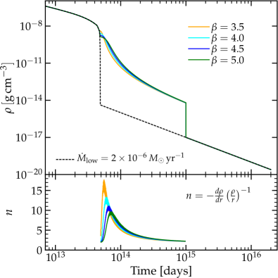
In the top panel of Figure 14, we show the density profiles of the models considered in this section. As was mentioned in Section 3.1, the high density CSM in these models is truncated at the radius $10^{15}\,{\rm cm}$. Above this radius, we attach a low density RSG wind with the mass loss rate $\dot{M}=2.0\times 10^{-6}\,M_{\odot}\,{\rm yr}^{-1}$. For comparison, the black dashed line in the top panel of Figure 14 shows the model with low density wind only. When constructing the models shown in Figure 14, we imposed the condition of constant total CSM mass, $M_{\rm CSM}=0.5\,M_{\odot}$, as in the previous section. Our motivation for it is based on the roughly equal amount of mass needed to reproduce the early light curve of another SN, 2013fs, by the models including steady ($0.47\,M_{\odot}$, Morozova et al. 2017a) and accelerating ($0.5\,M_{\odot}$, Moriya et al. 2017) high density winds. The bottom panel of Figure 14 shows the slope $n$ in the CSM of the corresponding models from top panel, computed as $n=-(d\rho/dr)r/\rho$, as a function of $r$. In this plot, one can see that in this kind of CSM the density declines with radius rather steeply, with the values of $n$ comparable to the ones from our Section 5 and larger in some regions .

Figure 14.— Top panel: Density profiles of the models with CSM constructed in a way similar to Moriya et al. (2017, 2018), where it represents accelerating wind. For comparison, black dashed line shows the model with low density wind only. Bottom panel: Slopes of the corresponding CSM profiles from the top panel as a function of radial coordinate.

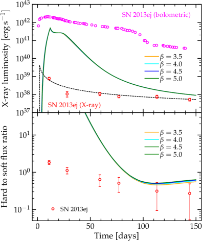
In the top panel of Figure 15, we show the X-ray signal obtained from these models using numerical approach outlined in Sections 3.2 and 3.3, and compare it to the observed X-ray signal from SN 2013ej. The final energy of the models is $0.68\,{\rm B}$ in all cases. We transform the flux into luminosity (multiplying by $4\pi$ times distance to SN 2013ej squared) and plot it together with the X-ray and quasi-bolometric luminosities of SN 2013ej (for the quasi-bolometric luminosity, see Valenti et al., 2016). This plot shows that the X-ray flux we obtain from the models with accelerating wind is few orders of magnitude larger than the observed X-ray flux in the first $\sim 50$ days, and its luminosity is almost comparable to the quasi-bolometric luminosity of SN 2013ej. The light curves from the models with different values of $\beta$ are very close to each other and nearly indistinguishable in the plot. For reference, the black dashed curve shows the X-ray signal from the model with low density wind of the mass loss rate $\dot{M}=2.0\times 10^{-6}\,M_{\odot}\,{\rm yr}^{-1}$ only (the same as blue curve in the top panel of Figure 9). The bottom panel of Figure 15 shows the ratio between hard ($2.0-8.0\,{\rm keV}$) and soft ($0.5-2.0\,{\rm keV}$) components of the obtained X-ray signal, compared to the values observed in SN 2013ej.

Figure 15.— Top panel: X-ray luminosity obtained from the models shown in Figure 14. The curves corresponding to the different values of $\beta$ are nearly identical. Black dashed line shows the X-ray signal from the model with low density wind only (mass loss rate $\dot{M}=2.0\times 10^{-6}\,M_{\odot}\,{\rm yr}^{-1}$). For comparison, red markers show the luminosity of SN 2013ej in X-rays, and magenta markers show the quasi-bolometric luminosity of this SN derived from the optical observations (Valenti et al., 2016). Bottom panel: The ratio between hard ($2.0-8.0\,{\rm keV}$) and soft ($0.5-2.0\,{\rm keV}$) components of the obtained X-ray signal, compared to the values observed in SN 2013ej.

Figure 16.— Evolution of the temperature profile (top panel), the density profile (middle panel), and the X-ray emission from each grid cell (bottom panel) of the forward and reverse shock waves in $\beta=5$ model from Figure 14.

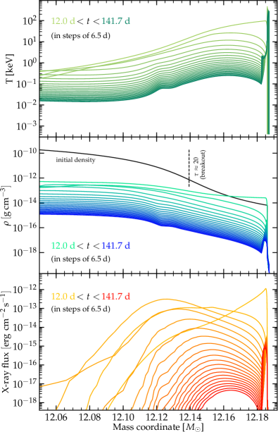
In order to identify the source of excessive X-ray emission seen in Figure 15, we plot the hydrodynamical evolution of the $\beta=5$ model from Figure 14 in Figure 16. The top panel of Figure 16 shows the temperature evolution in the outer $\sim$$0.15\,M_{\odot}$ of the CSM between days $12$ and $142$ (by the day $12$, the shock breakout in this model has already happened). This plot demonstrates that the outer layer of this CSM gets heated by the original post-explosion shock wave to very high temperatures, of the order of a keV and larger. Subsequently, after the shock wave has reached the boundary between the CSM and the low density wind, it gives rise to the usual forward/reverse shock wave pattern, similar to the one from Figure 2, jammed along the right hand side of Figure 16 (note different range of the mass coordinate in these figures).

The middle panel of Figure 16 illustrates the evolution of density in this model. For reference, we plot the initial density profile with a solid black line. The velocity of matter ($v$) in the outer layer of this CSM is $\sim$$15,000\,{\rm km}\,{\rm s}^{-1}$ in our simulations, therefore we estimate that the shock breakout in this model should happen at the optical depth $\tau\approx c/v\approx 20$, where $c$ is the speed of light. We calculate the optical depth in the CSM by finding the integral $\tau=\int_{r}^{R_{\rm CSM}}\kappa\rho dr$, where the opacity $\kappa$ is equal to $0.34\,{\rm cm}^{2}\,{\rm g}^{-1}$. In the middle panel of Figure 16, we mark the location of shock breakout by a thin dashed line. To the right of this line, we expect that the temperature of matter will be affected by the radiative cooling during the shock breakout. However, to the left of this line, the radiation will be trapped before the breakout, and the matter will be able to reach the temperatures shown in the top panel of Figure 16.

The bottom panel of Figure 16 shows total X-ray flux from each numerical grid cell of the $\beta=5$ model. It demonstrates that in the first $\sim$$40-50$ days of the evolution the X-ray emission from this model is dominated by the outer $0.1\,M_{\odot}$ of the CSM, due to its high temperature and relatively high density. Note that in this plot we show the X-ray flux already after accounting for the absorption by all material outer to a given cell, and only in the energy range $0.5-8.0\,{\rm keV}$. This explain very large X-ray emission from this model seen in Figure 15. After day $\sim$$50$, the reverse shock wave reflected at the boundary between the CSM and the low density wind becomes the dominant source of the X-ray signal. By the end of the simulation, at day $\sim$$150$, the X-ray flux from this model almost entirely comes from the outer shocked ejecta, as in the cases described in Sections 4 and 5.

It is important to note that the X-ray emission seen in the bottom panel of Figure 16 comes from the outermost region of the CSM, which quickly becomes optically thin (within the first few tens of days after the breakout). Therefore, it cannot be captured by the codes (both gray and multigroup), which track the diffusion of radiation from the inner ejecta regions either up to the photosphere, or to the point where the radiation decouples from the matter. In order to properly describe this X-ray emission, one needs to look at the temperature across the entire model, including the optically thin regions.

On the other hand, our numerical simulations use a range of assumptions, which likely lead to the overestimate of the temperature in CSM. Perhaps, the most important of those is neglecting the radiative cooling. In order to check how the radiative cooling by X-rays may affect our results, we performed test simulations similar to the one in Section 4.3, employing the cooling function $\Lambda$ from Equation (6). This formula estimates the total loss of energy due to free-free (dominates at the temperatures $T\gtrsim 2.6\times 10^{7}$) and bound-free (dominates at the temperatures $T\lesssim 2.6\times 10^{7}$) X-ray emission (Chevalier & Fransson, 2016). In Section 4.3, we subtracted the entire amount of this energy from the shocked ejecta, without taking into account that part of it may be reabsorbed by the matter. Nevertheless, the resulting X-ray light curve was only slightly affected by the cooling (see Figure 8). However, the hydrogen column of the CSM in this section is much larger than the hydrogen column of the shocked ejecta in Section 4.3, and part of the emitted energy will be inevitably reabsorbed back.

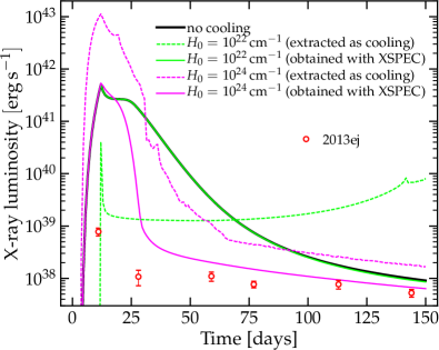
To roughly account for the reabsorption, we multiply $\Lambda$ by the factor $\exp(-H/H_{0})$, where $H$ is the hydrogen column at a given point (see Section 3.3 for the definition) and $H_{0}$ is its characteristic value. Specifically, we apply the cooling function at each time step by adding the term $-\exp(-H/H_{0})\Lambda n_{e}n_{i}dt$ to the energy density in all grid cells, where the temperature is higher than $5\times 10^{4}\,{K}$. We perform the simulations with two values of $H_{0}$, $10^{22}$ and $10^{24}\,{\rm cm}^{-1}$, and record the amount of energy extracted from the model in each case. After that, we analyse these simulations with XSPEC and compare the obtained X-ray light curve to the extracted energy. This approach is not self-consistent, but it helps us understand whether we subtract the right amount of energy from the model or not.

Figure 17 summarizes the results of this test for the $\beta=5$ model from Figure 14. The black solid line shows the light curve obtained without radiative cooling. Comparing solid and dashed green lines for the model with $H_{0}=10^{22}\,{\rm cm}^{-1}$, we can see that our cooling method does not remove a sufficient amount of energy in this simulation during the first $\sim$$70$ days, therefore, the X-ray light curve stays the same as in the case without cooling. The fact that after this time the dashed green line is much higher than the solid green line does not contradict to this, because the X-ray emission in that period is already dominated by the reverse shock wave, which is weakly affected by the cooling (see Section 4.3), and the energy given by green dashed line come from the deeper regions, which do not contribute much to the signal anymore. Instead, comparing solid and dashed magenta lines for the simulation with $H_{0}=10^{24}\,{\rm cm}^{-1}$, we can see that in this case we remove more energy from the model than necessary, and the X-ray light curve does become weaker. Nevertheless, it stays excessively large in the first $\sim$$30$ days. This suggests that the correct X-ray signal from this model may lie between the solid magenta and the solid green curves. However, this needs to be shown in more accurate numerical models of the X-ray emission.

Figure 17.— X-ray light curves obtained from the $\beta=5$ model with radiative cooling (green and magenta solid lines), compared to the total amount of energy extracted from the corresponding hydro simulations (green and magenta dashed lines). The black line shows the X-ray light curve from the model without cooling. The plot shows that in the case of $H_{0}=10^{22}\,{\rm cm}^{-1}$ we do not subtract enough energy from the model, while in the case of $H_{0}=10^{24}\,{\rm cm}^{-1}$ we subtract more energy than necessary. We conclude that the correct X-ray light curve from this model likely lies between the solid green and solid magenta curves.

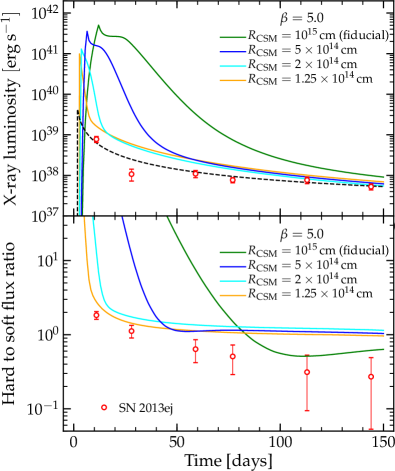
Finally, in Figure 18, we check the dependence of our results on the size of the dense CSM with varying slope. For this test, we focus on the $\beta=5$ model from Figure 14 and truncate it at the radii $R_{\rm CSM}=5\times 10^{14}\,{\rm cm}$, $2\times 10^{14}\,{\rm cm}$, and $1.25\times 10^{14}\,{\rm cm}$, where the latter value is equal to the size of the best fitting constant slope CSM model from Section 5 ($1800\,R_{\odot}$). Above the truncated dense CSM, we attach the $\dot{M}=2.0\times 10^{-6}\,M_{\odot}\,{\rm yr}^{-1}$ low density wind as we did before. The top panel of Figure 18 demonstrates that the excessive X-ray signal from the $\beta=5$ model is very sensitive to the size of the dense CSM, and it nearly vanishes for the smaller valuer of $R_{\rm CSM}$. In Moriya et al. (2017, 2018), the value of $R_{\rm CSM}=10^{15}\,{\rm cm}$ was chosen somewhat arbitrarily, but the top panel of Figure 18 suggests that the X-ray signal from SNe II, or the absence of such signal, may put a constraint on the size of the dense CSM and, therefore, on the duration of its formation.

However, using the smaller CSM radii of the $\beta=5$ model, we nevertheless cannot achieve a good agreement with the observed hardness of the X-ray signal from SN 2013ej. The bottom panel of Figure 18 shows the ratio between the hard and soft components of the X-ray flux, from which we can see that the models overestimate the observed temperatures. This can be naturally explained by the fact that trimming the CSM in the $\beta=5$ model we make it more similar to the models from Section 5. In those models, the X-ray signal, instead of being dominated by the outermost overheated region of the CSM, mainly comes from the reverse shock wave formed at the boundary between the dense CSM and the low density wind. The results of Section 5 (see Figure 11) suggest that the hardness of this X-ray signal depends on the velocity of the ejecta, which, in turn, is determined by the CSM slope. And indeed, because the slope of the $\beta=5$ model reaches the values of $\sim$7 and higher (Figure 14), the hardness of its X-ray emission seen in the bottom panel of Figure 18 is remarkably similar to the hardness seen in Figure 11 for the models with $n=7$ and $n=8$. This once again emphasizes the importance of the CSM slope in reproducing the right temperature of the observed X-ray signal. In addition, we obtained the optical light curve from the $\beta=5$ model trimmed to the radius $R_{\rm CSM}=1.25\times 10^{14}\,{\rm cm}$ using SNEC, and found that it is almost identical to the ligth curve from the $n=8$ model of Section 5.

Figure 18.— Top panel: X-ray luminosity obtained from the $\beta=5$ model truncated at the CSM radii of $R_{\rm CSM}=5\times 10^{14}\,{\rm cm}$, $2\times 10^{14}\,{\rm cm}$, and $1.25\times 10^{14}\,{\rm cm}$. Black dashed line shows the X-ray signal from the model with low density wind only (mass loss rate $\dot{M}=2.0\times 10^{-6}\,M_{\odot}\,{\rm yr}^{-1}$). For comparison, red markers show the observed X-ray luminosity of SN 2013ej. Bottom panel: The ratio between hard ($2.0-8.0\,{\rm keV}$) and soft ($0.5-2.0\,{\rm keV}$) components of the X-ray signal from the $\beta=5$ model with reduced CSM radii.

Due to the assumptions we use in our analysis, the results we obtain in this section by no means can rule out the models of accelerating wind, or question their validity. More detailed simulations, taking into account radiative cooling, Comptonization of the optical photons, and incomplete equipartition between the ions and electrons, are needed in order to have a more clear picture of the X-ray emission from these models. Nevertheless, this simplistic approach shows that the early SN II observations in X-ray can play an important role in constraining the properties of this kind of CSM. Even is the excessive heating we see in these models is entirely eliminated by the radiative cooling, the question of whether the outer layers of this CSM are accelerated to the right velocities in order to ensure the right temperature in the reverse shock wave (and, consequently, correct X-ray spectrum) still stays open. After all, if the models including dense CSM with varying slope (aka accelerating wind) indeed represent the right way to describe the pre-explosion configuration of SN II progenitors, more accurate numerical simulations of the X-ray signal from these models will confirm it by reproducing the early X-ray data observed in SNe II.

7. Conclusions

It goes without saying that a good SN model should reproduce observations across the entire electromagnetic spectrum, and for the core-collapse SNe II also in neutrinos (Murase, 2017; Seadrow et al., 2018) and gravitational waves (Morozova et al., 2018). This is a tremendously difficult problem, and the presence of a dense CSM of unknown nature makes it even more complicated. In this study, we attempted to find a model that could fit both optical photometry of SN 2013ej until the end of the plateau phase and its X-ray signal in the first $\sim$$150$ days. In order to accomplish this, we had to use a set of simplifying assumptions. Here, we summarize the conclusions of this work, which we think are robust.

• Inclusion of a dense CSM in the pre-explosion model changes the location of the forward/reverse shock waves responsible for most of the X-ray signal in SNe II. Instead of forming at the interface between the RSG surface and the low density wind, they form at the interface between the dense CSM and the low density wind. In this scenario, the reverse shock wave probes the outer edge of the dense CSM, while the forward shock wave propagates into the regular low density RSG wind. This may explain the fact that radio observations of SNe II favor low mass loss rates from their progenitors, similar to the regular mass loss rates of RSGs (Chevalier et al., 2006).

• The density slope in the CSM sets up the conditions for the acceleration of the original post-explosion shock wave. The steepness of this slope defines the final velocity of the outermost CSM layers, which, in turn, determines the temperature in the reverse shock wave and the observed X-ray spectrum. Steeper CSM profiles result in a harder X-ray emission. Therefore, while modeling SN optical photometry helps constraining the total CSM mass, modeling their X-ray signal may help constraining the CSM slope.

• We find that $\rho\propto r^{-2}$ (dense steady wind) CSM profile cannot accelerate the original shock wave enough to explain the ratio between the hard and soft X-ray components observed in SN 2013ej. More accurate treatment of radiative cooling would likely make the agreement worse. Instead, we show that a steeper, $\rho\propto r^{-5}$ CSM with the same total mass and radial extent does better job in reproducing optical and X-ray emission from SN 2013ej (see Figure 13 for the full set of parameters in this model).

• On the other hand, we find that steeper and more extended CSM profiles, similar to the $\beta$-law models of accelerating wind, may create conditions that lead to the excessive X-ray emission, which is not observed in SNe II. However, this conclusion is sensitive to the assumptions that we use and must be carefully checked by more detailed simulations. Nevertheless, we argue that reproducing X-ray signal from young SNe II is an important test that any viable CSM model should pass.

All simulations performed here assume spherical symmetry, but this assumption does not necessarily hold true in real SNe. In fact, the unusually strong polarization seen in the spectra of SN 2013ej (Leonard et al., 2013; Kumar et al., 2016) likely indicates a significant asymmetry in the ejecta. Due to their complexity and computational cost, multi-dimensional numerical simulations of aspherical CSM interactions are still not very common. Motivated by nebular observations of SN 1987A, Blondin et al. (1996) performed two- and three-dimensional simulations of a shock wave entering an axisymmetric CSM with the polar angle dependent density profile having minimum at the pole and maximum at the equator. They found that for a highly aspherical CSM the shock wave forms a protrusion along the axis up to $\sim$4 times larger than the main radius of the shock. Another approach was taken in the works of Couch et al. (2009); Suzuki et al. (2016); Afsariardchi & Matzner (2018), where the authors considered a spherically symmetric density profile, but employed an aspherical explosion mechanism to launch the shock wave. Under certain conditions, such setup may lead to the formation of an ‘oblique’ shock wave propagating along the stellar surface in the direction of the polar angle towards the equator. Jun et al. (1996) studied the enhancement of the Rayleigh-Taylor instability in a shock wave interacting with a clumpy CSM and suggested that the presence of clumps can lead to a stronger X-ray and radio signal.

In addition to possible asphericity of the density profile or the explosion mechanism, a spherically symmetric shock wave accelerating in a steep density profile may become unstable with respect to small linear perturbations (Goodman, 1990; Chevalier, 1990). For example, Sari et al. (2000) found that in the case of an adiabatic equation of state with $\gamma=5/3$ the minimum density slope at which the accelerating shock wave becomes unstable is $n_{c}\approx 7.7$. This fact could be especially relevant for the CSM models from Section 6 with small values of $\beta$, where the slopes may reach values much higher than $n_{c}$ (see Figure 14). Without detailed multi-dimensional numerical simulations it is very hard to say how the effects of asphericity, clumpiness, and shock wave instability will influence the results of our study. In the future, we hope to be able to perform such simulations and address this question.

This study focused on a single well-observed object, but analysis of a larger sample of X-ray bright SNe II would give us much better idea on the variety of CSM around RSGs and could potentially help clarifying its origin. In this view, we encourage observational programs of young SNe II using current and future X-ray facilities (Chakraborti et al., 2012, 2013, 2016; Ross & Dwarkadas, 2017) and anticipate exciting results that will be obtained with those data.

References

- Afsariardchi & Matzner (2018) Afsariardchi, N., & Matzner, C. D. 2018, ApJ, 856, 146
- Anderson et al. (2014) Anderson, J. P., González-Gaitán, S., Hamuy, M., et al. 2014, ApJ, 786, 67
- Andrews & Smith (2017) Andrews, J. E., & Smith, N. 2017, ArXiv e-prints
- Arnaud (1996) Arnaud, K. A. 1996, in Astronomical Society of the Pacific Conference Series, Vol. 101, Astronomical Data Analysis Software and Systems V, ed. G. H. Jacoby & J. Barnes, 17
- Arnett (1980) Arnett, W. D. 1980, ApJ, 237, 541
- Arnett & Fu (1989) Arnett, W. D., & Fu, A. 1989, ApJ, 340, 396
- Asplund et al. (2009) Asplund, M., Grevesse, N., Sauval, A. J., & Scott, P. 2009, ARA&A, 47, 481
- Bersten et al. (2011) Bersten, M. C., Benvenuto, O., & Hamuy, M. 2011, ApJ, 729, 61
- Blinnikov (1996) Blinnikov, S. I. 1996, Astronomy Letters, 22, 79
- Blondin et al. (1996) Blondin, J. M., Lundqvist, P., & Chevalier, R. A. 1996, ApJ, 472, 257
- Boian & Groh (2017) Boian, I., & Groh, J. 2017, ArXiv e-prints
- Borkowski et al. (2001) Borkowski, K. J., Lyerly, W. J., & Reynolds, S. P. 2001, ApJ, 548, 820
- Borkowski et al. (1994) Borkowski, K. J., Sarazin, C. L., & Blondin, J. M. 1994, ApJ, 429, 710
- Bose et al. (2015) Bose, S., Sutaria, F., Kumar, B., et al. 2015, ApJ, 806, 160
- Bouret et al. (2005) Bouret, J.-C., Lanz, T., & Hillier, D. J. 2005, A&A, 438, 301
- Bullivant et al. (2018) Bullivant, C., Smith, N., Grant Williams, G., et al. 2018, MNRAS
- Burrows et al. (2016) Burrows, A., Vartanyan, D., Dolence, J. C., Skinner, M. A., & Radice, D. 2016, ArXiv e-prints
- Cedrés et al. (2012) Cedrés, B., Cepa, J., Bongiovanni, Á., et al. 2012, A&A, 545, A43
- Chakraborti et al. (2012) Chakraborti, S., Yadav, N., Ray, A., et al. 2012, ApJ, 761, 100
- Chakraborti et al. (2013) Chakraborti, S., Ray, A., Smith, R., et al. 2013, ApJ, 774, 30
- Chakraborti et al. (2016) —. 2016, ApJ, 817, 22
- Chevalier (1982) Chevalier, R. A. 1982, ApJ, 259, 302
- Chevalier (1990) —. 1990, ApJ, 359, 463
- Chevalier (2012) —. 2012, ApJ, 752, L2
- Chevalier & Fransson (1994) Chevalier, R. A., & Fransson, C. 1994, ApJ, 420, 268
- Chevalier & Fransson (2003) Chevalier, R. A., & Fransson, C. 2003, in Lecture Notes in Physics, Berlin Springer Verlag, Vol. 598, Supernovae and Gamma-Ray Bursters, ed. K. Weiler, 171–194
- Chevalier & Fransson (2016) —. 2016, ArXiv e-prints
- Chevalier et al. (2006) Chevalier, R. A., Fransson, C., & Nymark, T. K. 2006, ApJ, 641, 1029
- Chugai et al. (2007) Chugai, N. N., Chevalier, R. A., & Utrobin, V. P. 2007, ApJ, 662, 1136
- Cohen et al. (2011) Cohen, D. H., Gagné, M., Leutenegger, M. A., et al. 2011, MNRAS, 415, 3354
- Cohen et al. (2010) Cohen, D. H., Leutenegger, M. A., Wollman, E. E., et al. 2010, MNRAS, 405, 2391
- Couch et al. (2009) Couch, S. M., Wheeler, J. C., & Milosavljević, M. 2009, ApJ, 696, 953
- Das & Ray (2017) Das, S., & Ray, A. 2017, ApJ, 851, 138
- de Jager et al. (1988) de Jager, C., Nieuwenhuijzen, H., & van der Hucht, K. A. 1988, A&AS, 72, 259
- Dessart et al. (2013) Dessart, L., Hillier, D. J., Waldman, R., & Livne, E. 2013, MNRAS, 433, 1745
- Dessart et al. (2017) Dessart, L., John Hillier, D., & Audit, E. 2017, A&A, 605, A83
- Dessart & Owocki (2005) Dessart, L., & Owocki, S. P. 2005, A&A, 437, 657
- Dhungana et al. (2013) Dhungana, G., Vinko, K., Wheeler, J. C., et al. 2013, Central Bureau Electronic Telegrams, 3609
- Dhungana et al. (2016) Dhungana, G., Kehoe, R., Vinko, J., et al. 2016, ApJ, 822, 6
- Dwarkadas (2014) Dwarkadas, V. V. 2014, MNRAS, 440, 1917
- Dwarkadas et al. (2010) Dwarkadas, V. V., Dewey, D., & Bauer, F. 2010, MNRAS, 407, 812
- Dwarkadas & Gruszko (2012) Dwarkadas, V. V., & Gruszko, J. 2012, MNRAS, 419, 1515
- Faran et al. (2014a) Faran, T., Poznanski, D., Filippenko, A. V., et al. 2014a, MNRAS, 445, 554
- Faran et al. (2014b) —. 2014b, MNRAS, 442, 844
- Ferguson et al. (2005) Ferguson, J. W., Alexander, D. R., Allard, F., et al. 2005, ApJ, 623, 585
- Förster et al. (2016) Förster, F., Maureira, J. C., San Martín, J., et al. 2016, ApJ, 832, 155
- Fransson (1984) Fransson, C. 1984, A&A, 133, 264
- Fraser et al. (2014) Fraser, M., Maund, J. R., Smartt, S. J., et al. 2014, MNRAS, 439, L56
- Fuller (2017) Fuller, J. 2017, MNRAS, 470, 1642
- Fullerton et al. (2006) Fullerton, A. W., Massa, D. L., & Prinja, R. K. 2006, ApJ, 637, 1025
- Gal-Yam et al. (2014) Gal-Yam, A., Arcavi, I., Ofek, E. O., et al. 2014, Nature, 509, 471
- Ganot et al. (2016) Ganot, N., Gal-Yam, A., Ofek, E. O., et al. 2016, ApJ, 820, 57
- Gardiner & Stone (2005) Gardiner, T. A., & Stone, J. M. 2005, Journal of Computational Physics, 205, 509
- Gardiner & Stone (2008) —. 2008, Journal of Computational Physics, 227, 4123
- Gezari et al. (2015) Gezari, S., Jones, D. O., Sanders, N. E., et al. 2015, ApJ, 804, 28
- Goldman et al. (2017) Goldman, S. R., van Loon, J. T., Zijlstra, A. A., et al. 2017, MNRAS, 465, 403
- Goodman (1990) Goodman, J. 1990, ApJ, 358, 214
- Guillochon et al. (2017) Guillochon, J., Parrent, J., Kelley, L. Z., & Margutti, R. 2017, ApJ, 835, 64
- Gutiérrez et al. (2017) Gutiérrez, C. P., Anderson, J. P., Hamuy, M., et al. 2017, ApJ, 850, 89
- Hicken et al. (2017) Hicken, M., Friedman, A. S., Blondin, S., et al. 2017, ApJS, 233, 6
- Hosseinzadeh et al. (2018) Hosseinzadeh, G., Valenti, S., McCully, C., et al. 2018, ArXiv e-prints
- Huang et al. (2015) Huang, F., Wang, X., Zhang, J., et al. 2015, ApJ, 807, 59
- Iglesias & Rogers (1996) Iglesias, C. A., & Rogers, F. J. 1996, ApJ, 464, 943
- Immler (2007) Immler, S. 2007, in American Institute of Physics Conference Series, Vol. 937, Supernova 1987A: 20 Years After: Supernovae and Gamma-Ray Bursters, ed. S. Immler, K. Weiler, & R. McCray, 246–255
- Johnson et al. (2017) Johnson, S. A., Kochanek, C. S., & Adams, S. M. 2017, ArXiv e-prints
- Jun et al. (1996) Jun, B.-I., Jones, T. W., & Norman, M. L. 1996, ApJ, 468, L59
- Kalberla et al. (2005) Kalberla, P. M. W., Burton, W. B., Hartmann, D., et al. 2005, A&A, 440, 775
- Khazov et al. (2016) Khazov, D., Yaron, O., Gal-Yam, A., et al. 2016, ApJ, 818, 3
- Kiewe et al. (2012) Kiewe, M., Gal-Yam, A., Arcavi, I., et al. 2012, ApJ, 744, 10
- Kim et al. (2013) Kim, M., Zheng, W., Li, W., et al. 2013, Central Bureau Electronic Telegrams, 3606
- Kudritzki & Puls (2000) Kudritzki, R.-P., & Puls, J. 2000, ARA&A, 38, 613
- Kumar et al. (2016) Kumar, B., Pandey, S. B., Eswaraiah, C., & Kawabata, K. S. 2016, MNRAS, 456, 3157
- Lee et al. (2013) Lee, M., Li, K. L., Wang, J.-W., et al. 2013, The Astronomer’s Telegram, 5466
- Leonard et al. (2013) Leonard, P. b. D. C., Pignata, G., Dessart, L., et al. 2013, The Astronomer’s Telegram, 5275
- Litvinova & Nadezhin (1983) Litvinova, I. I., & Nadezhin, D. K. 1983, Ap&SS, 89, 89
- Margutti et al. (2013) Margutti, R., Chakraborti, S., Brown, P. J., & Sokolovsky, K. 2013, The Astronomer’s Telegram, 5243
- Mauerhan et al. (2013) Mauerhan, J. C., Smith, N., Filippenko, A. V., et al. 2013, MNRAS, 430, 1801
- McDowell et al. (2018) McDowell, A. T., Duffell, P. C., & Kasen, D. 2018, ArXiv e-prints
- Moriya et al. (2011) Moriya, T., Tominaga, N., Blinnikov, S. I., Baklanov, P. V., & Sorokina, E. I. 2011, MNRAS, 415, 199
- Moriya et al. (2018) Moriya, T. J., Förster, F., Yoon, S.-C., Gräfener, G., & Blinnikov, S. I. 2018, MNRAS
- Moriya et al. (2017) Moriya, T. J., Yoon, S.-C., Gräfener, G., & Blinnikov, S. I. 2017, MNRAS, 469, L108
- Morozova et al. (2016) Morozova, V., Piro, A. L., Renzo, M., & Ott, C. D. 2016, ApJ, 829, 109
- Morozova et al. (2015) Morozova, V., Piro, A. L., Renzo, M., et al. 2015, ApJ, 814, 63
- Morozova et al. (2017a) Morozova, V., Piro, A. L., & Valenti, S. 2017a, ApJ, 838, 28
- Morozova et al. (2017b) —. 2017b, ArXiv e-prints
- Morozova et al. (2018) Morozova, V., Radice, D., Burrows, A., & Vartanyan, D. 2018, ArXiv e-prints
- Müller et al. (2012) Müller, B., Janka, H.-T., & Marek, A. 2012, ApJ, 756, 84
- Murase (2017) Murase, K. 2017, ArXiv e-prints
- Nagy et al. (2014) Nagy, A. P., Ordasi, A., Vinkó, J., & Wheeler, J. C. 2014, A&A, 571, A77
- Nagy & Vinkó (2016) Nagy, A. P., & Vinkó, J. 2016, A&A, 589, A53
- Nakaoka et al. (2018) Nakaoka, T., Kawabata, K. S., Maeda, K., et al. 2018, ApJ, 859, 78
- Nakar & Sari (2010) Nakar, E., & Sari, R. 2010, ApJ, 725, 904
- Nieuwenhuijzen & de Jager (1990) Nieuwenhuijzen, H., & de Jager, C. 1990, A&A, 231, 134
- Nymark et al. (2006) Nymark, T. K., Fransson, C., & Kozma, C. 2006, A&A, 449, 171
- Ofek (2014) Ofek, E. O. 2014, MATLAB package for astronomy and astrophysics, Astrophysics Source Code Library
- Ofek et al. (2014) Ofek, E. O., Sullivan, M., Shaviv, N. J., et al. 2014, ApJ, 789, 104
- Owocki & Puls (1999) Owocki, S. P., & Puls, J. 1999, ApJ, 510, 355
- Paczyński (1983) Paczyński, B. 1983, ApJ, 267, 315
- Pastorello et al. (2008) Pastorello, A., Quimby, R. M., Smartt, S. J., et al. 2008, MNRAS, 389, 131
- Patnaude et al. (2015) Patnaude, D. J., Lee, S.-H., Slane, P. O., et al. 2015, ApJ, 803, 101
- Patnaude et al. (2017) —. 2017, ApJ, 849, 109
- Paxton et al. (2018) Paxton, B., Schwab, J., Bauer, E. B., et al. 2018, ApJS, 234, 34
- Puls et al. (2006) Puls, J., Markova, N., Scuderi, S., et al. 2006, A&A, 454, 625
- Puls et al. (2008) Puls, J., Vink, J. S., & Najarro, F. 2008, A&A Rev., 16, 209
- Pumo et al. (2017) Pumo, M. L., Zampieri, L., Spiro, S., et al. 2017, MNRAS, 464, 3013
- Quataert & Shiode (2012) Quataert, E., & Shiode, J. 2012, MNRAS, 423, L92
- Radice et al. (2017) Radice, D., Burrows, A., Vartanyan, D., Skinner, M. A., & Dolence, J. C. 2017, ArXiv e-prints
- Ramírez-Agudelo et al. (2017) Ramírez-Agudelo, O. H., Sana, H., de Koter, A., et al. 2017, A&A, 600, A81
- Richmond (2014) Richmond, M. W. 2014, Journal of the American Association of Variable Star Observers (JAAVSO), 42, 333
- Ross & Dwarkadas (2017) Ross, M., & Dwarkadas, V. V. 2017, AJ, 153, 246
- Sari et al. (2000) Sari, R., Waxman, E., & Shvarts, D. 2000, ApJS, 127, 475
- Schlegel (2006) Schlegel, E. M. 2006, in IAU Symposium, Vol. 230, Populations of High Energy Sources in Galaxies, ed. E. J. A. Meurs & G. Fabbiano, 252–258
- Seadrow et al. (2018) Seadrow, S., Burrows, A., Vartanyan, D., Radice, D., & Skinner, M. A. 2018, ArXiv e-prints
- Shappee et al. (2013) Shappee, B. J., Kochanek, C. S., Stanek, K. Z., et al. 2013, The Astronomer’s Telegram, 5237
- Shiode & Quataert (2014) Shiode, J. H., & Quataert, E. 2014, ApJ, 780, 96
- Smith (2014) Smith, N. 2014, ARA&A, 52, 487
- Smith et al. (2015) Smith, N., Mauerhan, J. C., Cenko, S. B., et al. 2015, MNRAS, 449, 1876
- Smith et al. (2001) Smith, R. K., Brickhouse, N. S., Liedahl, D. A., & Raymond, J. C. 2001, ApJ, 556, L91
- Sokolovsky et al. (2013) Sokolovsky, K., Giroletti, M., Stagni, M., Nanni, M., & Mahabal, A. 2013, The Astronomer’s Telegram, 5264
- Stone et al. (2008) Stone, J. M., Gardiner, T. A., Teuben, P., Hawley, J. F., & Simon, J. B. 2008, ApJS, 178, 137
- Sukhbold et al. (2016) Sukhbold, T., Ertl, T., Woosley, S. E., Brown, J. M., & Janka, H.-T. 2016, ApJ, 821, 38
- Sukhbold & Woosley (2014) Sukhbold, T., & Woosley, S. E. 2014, ApJ, 783, 10
- Summa et al. (2016) Summa, A., Hanke, F., Janka, H.-T., et al. 2016, ApJ, 825, 6
- Sundqvist & Owocki (2013) Sundqvist, J. O., & Owocki, S. P. 2013, MNRAS, 428, 1837
- Suwa et al. (2016) Suwa, Y., Yamada, S., Takiwaki, T., & Kotake, K. 2016, ApJ, 816, 43
- Suzuki et al. (2016) Suzuki, A., Maeda, K., & Shigeyama, T. 2016, ApJ, 825, 92
- Taddia et al. (2013) Taddia, F., Stritzinger, M. D., Sollerman, J., et al. 2013, A&A, 555, A10
- Tanaka et al. (2016) Tanaka, M., Tominaga, N., Morokuma, T., et al. 2016, ApJ, 819, 5
- Utrobin & Chugai (2017) Utrobin, V. P., & Chugai, N. N. 2017, MNRAS, 472, 5004
- Valenti et al. (2013) Valenti, S., Sand, D., Howell, D. A., et al. 2013, Central Bureau Electronic Telegrams, 3609
- Valenti et al. (2014) Valenti, S., Sand, D., Pastorello, A., et al. 2014, MNRAS, 438, L101
- Valenti et al. (2016) Valenti, S., Howell, D. A., Stritzinger, M. D., et al. 2016, MNRAS, 459, 3939
- Vink et al. (2001) Vink, J. S., de Koter, A., & Lamers, H. J. G. L. M. 2001, A&A, 369, 574
- Weaver et al. (1978) Weaver, T. A., Zimmerman, G. B., & Woosley, S. E. 1978, ApJ, 225, 1021
- Woosley & Heger (2007) Woosley, S. E., & Heger, A. 2007, Phys. Rep., 442, 269
- Woosley & Heger (2015) —. 2015, ApJ, 810, 34
- Wright & Barlow (1975) Wright, A. E., & Barlow, M. J. 1975, MNRAS, 170, 41
- Yaron et al. (2017) Yaron, O., Perley, D. A., Gal-Yam, A., et al. 2017, Nature Physics, 13, 510
- Yuan et al. (2016) Yuan, F., Jerkstrand, A., Valenti, S., et al. 2016, MNRAS, 461, 2003
- Zaghloul et al. (2000) Zaghloul, M. R., Bourham, M. A., & Doster, J. M. 2000, J. Phys. D Appl. Phys., 33, 977
- Zhang et al. (2014) Zhang, J., Wang, X., Mazzali, P. A., et al. 2014, ApJ, 797, 5