Nonlinear system modeling based on
constrained Volterra series estimates

Abstract

A simple nonlinear system modeling algorithm designed to work with limited a priori knowledge and short data records, is examined. It creates an empirical Volterra series-based model of a system using an $l_{q}$-constrained least squares algorithm with $q\geq 1$. If the system $m\left(\cdot\right)$ is a continuous and bounded map with a finite memory no longer than some known $\tau$, then (for a $D$ parameter model and for a number of measurements $N$) the difference between the resulting model of the system and the best possible theoretical one is guaranteed to be of order $\sqrt{N^{-1}\ln D}$, even for $D\geq N$. The performance of models obtained for $q=1,1.5$ and $2$ is tested on the Wiener-Hammerstein benchmark system. The results suggest that the models obtained for $q>1$ are better suited to characterize the nature of the system, while the sparse solutions obtained for $q=1$ yield smaller error values in terms of input-output behavior.

I Introduction

We consider the following well-known problem: given limited prior knowledge about a discrete-time nonlinear dynamic system and a limited amount of noisy measurements $\left\{\left(u_{n},y_{n}\right)\right\},$ $n=1,\ldots,N,$ find an accurate model that describes the system’s behavior; [1]. The only important assumption we make on the system is that it is represented by a continuous map $m\left(\mathbf{u}_{n}\right)$, where $\mathbf{u}_{n}=[u_{n},\ldots,u_{n-\tau}]^{T}$, which has a finite memory, whose length is not specified but no larger than some $\tau\in\mathbb{N}$.

Such a system, for bounded input signals, can be approximated arbitrarily well by a double-truncated Volterra series model; cf. e.g. [2, 3, 4, 5, 6], [7] and the recent survey [10]. In practice, when no further information about the system is available, one would like to take the largest accessible model (limited only by the computational resources) to get the best possible approximation. Such an approach, in case of the Volterra representation, has however an immediate consequence: the number $D$ of model parameters is large even for models of moderate size. For the standard least squares approach this implies that, in order to estimate these parameters accurately from the noisy measurements of the system, the number of measurements $N$ should be much larger than $D$. In such a case, the corresponding computation routines become both time consuming and prone to numerical errors; see e.g. [2, 11, 12, 13, 1], [14], [15], [16]. The recent advances in statistics alleviate this issue by offering constrained optimization algorithms that produce models of good quality for a number of measurements $N$ comparable to (or even smaller than) the number of model parameters $D$. The constraint assumptions are mild and in this work they translate to the requirement that, for a given system, the $l_{q}$-norm, $q\geq 1$, of the vector composed of its Volterra representation coefficients is finite. Our modeling algorithm relies on constrained convex optimization techniques, [17, 18], and is derived from the aggregative algorithms which, for $q=1$, were proposed and examined in e.g. [19, 20], and then applied to dynamic nonlinear systems in [21].

The paper contribution consists in:

1. The class of nonlinear system modeling algorithms based on Volterra series and constrained optimization is examined for $l_{q}$ norms, $q\geq 1$.

2. The theoretical bounds for model errors are derived for finite $D$ and $N$. It is shown, in particular, that these errors grow like $\sqrt{\ln D}$ and vanishes like $\sqrt{N^{-1}}$ with growing $D$ and $N$, respectively; cf. e.g. [22, 23], where small sample size properties are also examined in nonlinear system modeling problems.

3. The practical performance was verified using the benchmark data from [24] and further investigated using the numerical experiment.

II Problem statement

The discrete-time nonlinear system of interest is described by the following input-output equation

$$y_{n}=m\left(\mathbf{u}_{n}\right)+e_{n}=m\left(u_{n},u_{n-1},\ldots,u_{n-\tau}\right)+e_{n},$$ (1)

where $u_{n}$ and $e_{n}$ are the input and the noise signals, respectively. The system is single-input single-output (SISO)  and $m\left(u_{n},u_{n-1},\ldots,u_{n-\tau}\right)$ denotes a nonlinear mapping whose output depends not only on the current input $u_{n}$ but also on the previous $\tau$ ones.

Figure 1: A nonlinear system.

About the signals and the system we assume that:

• The system input $u_{n}$ is a sequence of bounded i.i.d. random variables.

• The noise $e_{n}$ is a zero-mean i.i.d. random sequence with a finite variance, $\sigma^{2}<\infty$. The noise and the input are mutually independent sequences.

• The nonlinear system $m\left(\cdot\right)$ has a finite memory of a length which is unknown but no longer than some $\tau\in\mathbb{N}$. Moreover, $m\left(\cdot\right)$ is continuous and bounded, i.e. there is some $M_{m}>0$ for which $\left|m\left(\mathbf{u}_{n}\right)\right|\leq M_{m}$.

Assumptions A1 and A2 are typical for many system identification problems; cf. e.g. [1]. Assumption A3 says that our prior knowledge about the system is rather limited. We neither assume the knowledge of the system structure nor imply that there exists a specific parametric representation of any of its elements. The continuity requirement in A3 allows the system to be approximated by the Volterra series-based models; see also Remark 2.

Example 1.

Any LTI system with $\tau$-finite memory satisfies Assumption A3. It also holds true for the aforementioned e.g. block-oriented cascade (Hammerstein, Wiener, Wiener-Hammerstein, etc.) or multibranched cascade (e.g. Uryson) systems with $\tau$-finite overall memory length of their dynamic blocks and with (at least) Lipschitz static nonlinearities.

Our goal is to find a good estimate of the system under Assumptions A1–A3 based on a double-truncated Volterra series model

$$V\left(\mathbf{u}_{n}\right) = h_{0}+H_{1L}\left(\mathbf{u}_{n}\right)+\cdots+H_{PL}\left(\mathbf{u}_{n}\right)$$

$$= h_{0}+\sum_{p=1}^{P}H_{pL}\left(\mathbf{u}_{n}\right),$$

where $h_{0}$ is a constant and $H_{pL}\left(\mathbf{u}_{n}\right)$ are the truncated Volterra operators (see e.g. [2, 3, 5])

$$H_{pL}\left(\mathbf{u}_{n}\right)=\sum_{k_{1}=0}^{L-1}\cdots\sum_{k_{p}=0}^{L-1}h_{k_{1}\ldots k_{p}}\cdot\prod_{i=1}^{p}u_{n-k_{i}},$$

and where $h_{k_{1}\ldots k_{p}}$ are the $p$th order Volterra kernels; $P$ denotes the degree of the expansion and $L\leq\tau$ stands for the memory length of the model.

The Volterra expansion is derived from the Taylor series, see e.g. [8, Ch. 2.1], [9, Ch. 1.4] and extends its modeling capabilities by incorporating dynamics into models. It however does not expand the modeling capability w.r.t. nonlinearities. For the Volterra series, the class of admissible nonlinearities appears, in fact, to be smaller as indicated by an example of the peak-hold operator given by Boyd and Chua in [3, p. 1152] (here in a discrete-time version):

$$y_{n}=\max_{k=0,1,\ldots}\left\{x_{n-k}\right\}.$$ (3)

The operator in (3) is continuous but has no fading memory property and thus (by virtue of their theorem [3, Th. 3]) cannot be approximated arbitrarily well by a Volterra series. This example shows that, in order to effectively model the nonlinear system by the Volterra series, the assumptions imposed on the system nonlinearity:

• cannot be, in general, considered separately from the dynamics, and need to be stronger than in case of static nonlinear systems and their Taylor expansion-based models, where, by virtue of the Weierstrass-Stone theorem, it suffices that the nonlinearity is continuous (if we want it to be approximated arbitrarily well - as it is the case in our paper) or is analytic (if we want to recover it fully). Nevertheless,

• in the particular case of systems satisfying Assumption A3, the continuity requirements is sufficient because of the systems’ finite memory.

Remark 2.

In a special case of block-oriented systems of known structure (like e.g. the Hammerstein, Wiener, Uryson, or LNL and NLN systems), where the Volterra kernels can be expressed in terms of impulse response coefficients of dynamic linear blocks and of derivatives of the static nonlinearities, the constraints imposed on these nonlinearities can also be equivalent to the Taylor series ones; cf. e.g. [8, Ch. 2.1.1] and [6].

III The algorithm

Thanks to the fact that the kernels $h_{k_{1}\ldots k_{p}}$ in (II) are symmetric with respect to the permutations of indices $k_{1}\ldots k_{p}$, the number of parameters $D$ to be estimated reduces from $\frac{L^{P+1}-1}{L-1}$ to $\binom{L+P}{L}$; cf. [6]. However, even for small $P$ and $L$, $D$ is a large number and might not be further reduced without additional information about the structure of the system; see e.g. [25, 6]. Moreover, even if the system structure was known, we would not be able to decide what parameters $P$ and $L$ should be used since, under Assumption A3, the class of systems is still too general to be exactly represented by Volterra models. Therefore, in such a scenario one would take the largest available dictionary and let the data select the best subset. This requires an algorithm which either:

• selects the largest (i.e. the most important) coefficients ([26, 27, 28]) or, at least,

• is robust against the effect of overparametrization (i.e. the excessive number of model parameters).

We will show that the presented algorithm offers the latter property and, in particular, works when $D>N$.

Remark 3.

Some system structures, e.g. the Hammerstein or Uryson ones, have structured or sparse Volterra representations [25, 6]. Nevertheless, we do not assume that the structure of the system is known and therefore we need an algorithm which will work in either case (note that the LASSO-based algorithms are designed to work when it is assumed a priori that the model has a sparse structure [28]).

For notation simplicity, we arrange the coefficients of the Volterra series kernels $h_{k_{1}\ldots k_{p}},$ $p=1,\ldots,P$, $k_{j}=0,\ldots,L-1$ and $j=0,\ldots,p$, from the model (II), into a vector $\mathbf{\theta}=\left[\theta_{1},\theta_{2},\dots,\theta_{D}\right]^{T}$ and denote the corresponding Volterra terms as $m_{i}\left(\mathbf{u}\right),$ $i=1,\ldots,D$. The collection $\left\{m_{i}\left(\mathbf{u}\right)\right\}$ will be referred to as a dictionary. Note that by Assumption A1 we have that $\left|m_{i}\left(\mathbf{u}\right)\right|\leq M_{d}$, for some $M_{d}>0.$

The system model is thus expressed as

$$\hat{m}(\mathbf{u};\mathbf{\hat{\theta})}=\sum_{i=1}^{D}\hat{\theta}_{i}m_{i}\left(\mathbf{u}\right),$$ (4)

where $\mathbf{\hat{\theta}}=[\hat{\theta}_{1},\hat{\theta}_{2},\dots,\hat{\theta}_{D}]^{T}$ is the empirical counterpart of the vector $\mathbf{\theta}$, obtained from the measurement set $\left\{\left(u_{n},y_{n}\right)\right\},$ $n=1,\ldots,N$, by minimization of the empirical quadratic criterion (note that the summation in (5) starts at $\tau+1$ since the first $\tau$ values of the input are not known):

$$\hat{Q}\left(\mathbf{\theta}\right)=\frac{1}{N-\tau}\sum_{i=\tau+1}^{N}\left[\hat{m}\left(\mathbf{u}_{i};\mathbf{\theta}\right)-y_{i}\right]^{2}.$$ (5)

with the following constraint imposed on the solution

$$\left\|\mathbf{\theta}\right\|_{q}\leq D^{\frac{1}{q}-1}\text{, for a given }q\geq 1.$$ (6)

Remark 4.

By virtue of the well-known relation between the $l_{q}$-norms

$$\left\|\mathbf{\theta}\right\|_{q}\leq\left\|\mathbf{\theta}\right\|_{1}\leq D^{1-\frac{1}{q}}\left\|\mathbf{\theta}\right\|_{q},$$ (7)

the constraint in (6) implies that $\left\|\mathbf{\theta}\right\|_{1}\leq 1$, which is a pivotal fact used in the proof of the theoretical behavior of the model $\hat{m}(\mathbf{u};\mathbf{\hat{\theta})}$, and cannot be relaxed in general. However, if it is known that the structure of the system has a sparse Volterra representation, that is, if $\mathbf{\theta}$ is $K$-sparse for some $K<D$, then the right-hand side inequality in (7) turns into $\left\|\mathbf{\theta}\right\|_{1}\leq K^{1-\frac{1}{q}}\left\|\mathbf{\theta}\right\|_{q}$. In this case, the constraint in (6) remains the same for $q=1$, but for $q>1$ it can be turned into a weaker one

$$\left\|\mathbf{\theta}\right\|_{q}\leq K^{\frac{1}{q}-1}.$$

Example 5.

For $q=1,1.5$ and $2$, the constraint (6) takes the forms

$$\left\|\mathbf{\theta}\right\|_{1}\leq 1\text{, }\left\|\mathbf{\theta}\right\|_{1.5}\leq\sqrt[3]{D^{-1}}\text{, and }\left\|\mathbf{\theta}\right\|_{2}\leq\sqrt{D^{-1}},$$

respectively.

Remark 6.

In case of Volterra series, the constraint in (6) means that the sequence of Volterra kernel coefficients $\theta$ is in the space $l_{q}$, that is, they are $l_{q}$-summable. Note that this assumption is satisfied for all models with finite $P$ and $L$ (and for all $q\geq 1$) up to the multiplicative constant – see Section III-B and cf. Assumption A3. In turn, for the infinite memory models, it is satisfied if the system possesses a fading memory property; see [29]. Such a property holds, e.g. for Hammerstein, Wiener, Hammerstein-Wiener systems with Lipschitz nonlinearities and asymptotically stable linear subsystems; cf. Remark 2 and Example 1.

Figure 2: Possible selections of the tuning parameter (multiplication factor $R$) for $q=1$: (a) the optimal one (the smallest for which $\left\|\mathbf{\theta}^{\ast}\right\|_{1}=1$ holds); (b) too large $R$ can make the unconstrained LS solution acceptable; (c) too small $R$ can make the optimal solution $\mathbf{\theta}^{\ast}$ infeasible (black dot – LS solution, red – the optimal one $\mathbf{\theta}^{\ast}$, and white – the $l_{1}$ constrained empirical solution $\mathbf{\hat{\theta}}$).

III-A Theoretical properties

Here we present the main result of the paper, that is, the upper bound of the discrepancy between the empirical models (4) and the best possible one, given as

$$\hat{m}\left(\mathbf{u};\mathbf{\theta}^{\ast}\right)=\sum_{i=1}^{D}\theta_{i}^{\ast}m_{i}\left(\mathbf{u}\right),$$ (8)

where $\mathbf{\theta}^{\ast}$ is the solution to the following constrained least squares problem

$$\mathbf{\theta}^{\ast}=argmin_{\lVert\mathbf{\theta}\rVert_{q}\leq D^{1/q-1}}Q\left(\mathbf{\theta}\right),Q\left(\mathbf{\theta}\right)=E\left\{\hat{m}\left(\mathbf{u}_{n};\mathbf{\theta}\right)-y_{n}\right\}^{2},$$ (9)

for a given $q\geq 1$; cf. (5) and (6).

The theorem below gives the upper bound of this discrepancy and offers a formal justification of a good behavior of the examined models in case when $D$ is large and $D\geq N$.

Theorem 7.

Let the nonlinear system (1) fulfill Assumptions A1–A3 and let (6) hold for some $q=\chi\geq 1$, then, for any $q\in\left[1,\chi\right]$, the difference between the empirical model, $\hat{m}(\mathbf{u};\mathbf{\hat{\theta})}$, and the best possible one, $m\left(\mathbf{u};\mathbf{\theta}^{\ast}\right)$, has the following upper bound

$$E\{Q(\mathbf{\hat{\theta})\}}-Q\left(\mathbf{\theta}^{\mathbf{\ast}}\right)\leq C\cdot\frac{\sqrt{N}}{N-\tau}\sqrt{\left(\tau+1\right)\ln D},$$ (10)

for any $D>2,$ where $C=32\sqrt{e}(M\sigma+2M^{2})$ and $M=\max\left\{M_{m},M_{d}\right\}$.

Proof.

See Appendix. ∎

The theorem generalizes the result obtained in [21] for $q=1$ (see also the original one in [19]) and, in particular, says that:

• The upper bound of the error is practically immune to the number of model parameters $D$ as it grows only logarithmically with $D$. This property is of special significance for the Volterra series-based models, for which $D$ grows fast with both $L$ and $P$.

• For $D$ being of order equal to (or larger than) $\sqrt{N}$ (and hence for $D\geq N$), our models have the error upper bound lower than those produced by the unconstrained least squares algorithms, for which this bound is of order $D/N$; cf. e.g. [1].

Remark 8.

The exact value of $\tau$ is only needed to establish the formal bound of the error in (9). If $\tau$ is not known (or known to be infinite), then one should expect slightly worse performance of the algorithm – as shown for $q=1$ in [30] that if $\tau=\infty$, then the error bound vanishes slower (by a factor $\sqrt{\ln N}$) with growing $N$ and the additional term $N^{-c},c>0$ occurs.

Remark 9.

Assumptions A1-A3 can be slightly weakened. For instance, one can admit correlated input; see e.g. [21] for $q=1$. In that case, the resulting models error vanishes with growing $N$ and still maintain its robustness against large number of model parameters $D$ as in (10). The only drawback is that the overall memory length $\tau$ need to be increased in order to take into account the correlation of the signal. Also, the system memory does not need to be finite, however, the resulting error bound is larger as indicated in the Remark 8.

III-B Tuning the algorithm

Usually, we do not know a priori whether the constraint (6) is satisfied by the system of interest. Observe however that we can make any system satisfying the Assumption A3 compliant with (6) by multiplying the dictionary entries by some, sufficiently large, factor $R>0$. Below we shortly examine the impact of $R$ on the aggregation error bound in (10).

Figure 3: (a) Shapes and relative sizes of the constraint in (6) for $q=1$ (light grey), $q=1.5$ (white) and $q=2$ (dark gray); $D=2$; $\mathbf{\theta}^{\ast}=[1/2~{}1/2]$ (b) For a system with a ’sparse’ representation ($\mathbf{\theta}^{\ast}=[1~{}0]$), the dictionary entries, which are optimal for $q=1$, need to be, for $q=2$, multiplied by $R=\sqrt{2}$ (which is also equivalent to multiplying by $R$ the bound in (6)).

III-B1 Case $q=1$

For the $l_{1}$ constraint, $R$ has a quite straightforward impact on the aggregation error bound (10): its squared value occurs there as a multiplicative factor (see (15) in Remark 11 following the proof in Appendix 7 and cf. (10)):

$$C=32\sqrt{e}(RM\sigma+2\left(RM\right)^{2})$$ (11)

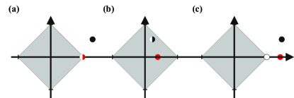
One would therefore like to make $R$ small, however, decreasing $R$ pushes the optimal solution $\mathbf{\theta}^{\mathbf{\ast}}$ towards the constraint boundary and can eventually set it outside of it; see the illustrations in Figs. 2a-c.

III-B2 Case $1<q\leq 2$

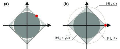
The left-hand side of the norm inequality in (7) indicates (and Fig. 3a illustrates it for $D=2$) that if for a given $q=\chi>1$, the constraint in (6) holds true for a system, then it holds for any other $q$’s such that $1\leq q<\chi$ and – consequently – the upper bound constants in (11) remain valid for all these $q$’s.

In the reversed situation, however, when it is only known that (6) holds for $q=1$, one needs to take $R=D^{1-\frac{1}{q}}$ (cf. the right-hand side of the inequality in (7) and Fig. 3b) to assure that (6) is valid for $q>1$ as well. This, unfortunately, can have a detrimental influence on the algorithm behavior since then

$$C=32\sqrt{e}(D^{1-\frac{1}{q}}M\sigma+2(D^{1-\frac{1}{q}}M)^{2})$$ (12)

and the upper bound of the aggregation error increases with $q$ and becomes approximately $D^{2(1-1/q)}$ times larger (i.e. up to $D$ times larger for $q=2$) than in (10).

III-B3 Empirical tuning algorithm

Below we propose a simple empirical algorithm to select a value of the tuning parameter $R$.

Algorithm: For a given $q\geq 1$, pick some (large) $R>0$, such that $\|\hat{\theta}\|_{q}\ll D^{\frac{1}{q}-1}$. Next, pick some (small) $\varepsilon>0$ and decrease $R$ until

$$\|\hat{\theta}\|_{q}\in[D^{\frac{1}{q}-1}-\varepsilon,D^{\frac{1}{q}-1}).$$

In the presence of noise one should usually decrease $R$ even more once $\|\hat{\theta}\|_{q}=D^{\frac{1}{q}-1}$ is attained, however, there is a risk that in such a case the actual solution $\theta^{\ast}$ will be shifted outside the constraint and a systematic (bias) error will be introduced; see Fig. 2c.

IV Experimental/simulation results

We first tested the algorithm on a real data example, namely the Wiener-Hammerstein benchmark presented in [24]. Then, to get a deeper insight into the behavior of the algorithm in a controlled environment, we also made additional experiments using a ’toy-example’ system with a Wiener-Hammerstein structure; the systems are referred to as WHB and WH2, respectively.

IV-A Wiener-Hammerstein benchmark

The benchmark data were taken from a nonlinear electronic system with a Wiener-Hammerstein structure, as depicted in Fig. 4. More details on how the benchmark data were generated can be found in [24].

Figure 4: The Wiener-Hammerstein benchmark system.

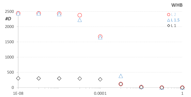
The system was modeled with a third degree Volterra series with varying (decreasing) memory lengths of each kernel, namely $L_{1}=80,$ $L_{2}=40$ and $L_{3}=20$. It resulted in the overall number of parameters $D=2441$. The measurement sets of lengths $N=500,1000,2000$ and $5000$ were taken from the benchmark’s learning data pool. Three models were estimated for $q=1,1.5$ and $2$. Algorithm III-B3 was used to tune the $R$ factor separately for each $q$; see Fig. 3.

Remark 10.

Decreasing the memory length in the consecutive Volterra kernels was dictated by the excessive computational overhead (the model with equal memory length kernels would have $\binom{80+3}{3}=\allowbreak 91\,881$ parameters) and the numerical issues encountered for the model of that size.

(a) First order Volterra kernels for $q=1,1.5,2$.

(b) Outputs of the system and its models for $q=1,2$.

Figure 5: WHB benchmark. Model kernels shapes and outputs comparison.

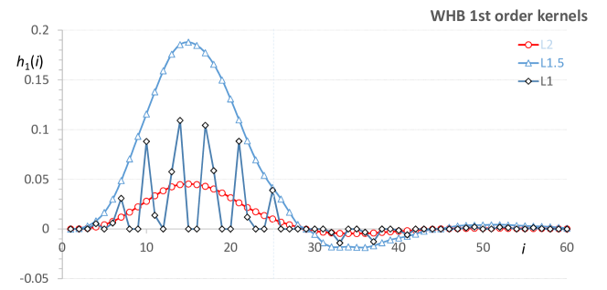
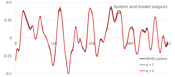
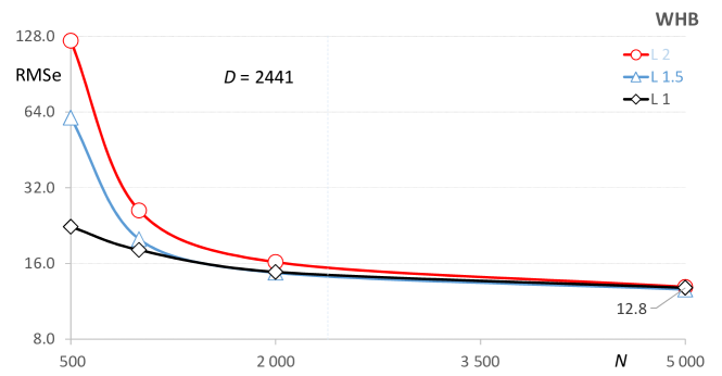
The experiments revealed that for each $N$ the model obtained for $q=1$ offered the smallest RMSe error (calculated according to the formula (4) in [24]) with respect to input-output behavior; see Fig. 6. It can be explained by its tendency to select a sparse representation; see Fig. 5 and 7; cf. e.g. [31, 33] and [28, Ch. 6].

(a) Model errors

(b) Model sparsities, i.e. the number of model coefficients greater than value on the $OX$ axis.

Figure 6: WHB benchmark. Comparison of model errors and their sparsities

IV-B Simulation example

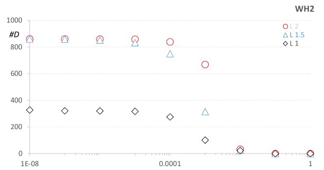
Let us now consider a system with the same Wiener-Hammerstein structure, but with the nonlinearity $x^{2}$, the input dynamics having the two-tap impulse response $\lambda_{0}=1$ and $\lambda_{1}=-1,$ and with the output dynamics having the following discrete transfer function $G\left(z\right)=0.2655z/\left(z^{2}-1.714z+0.78\right)$. The input signal $\left\{u_{n}\right\}$ was white and uniformly distributed in the interval $[-\sqrt{3},\sqrt{3}]$. The additive output noise was white and Gaussian, and was scaled in order to make the SNR = $1,10,40,80$ and $100$. The measurement sets had lengths $N=500,750,1000,1250,1500$ and $2000$. The Volterra model used in this experiment was the second order one with equal memory length kernels, $L_{1}=L_{2}=L=40$ (it thus had $D=861$ parameters).

The experiment was repeated to evaluate three models, for $q=1,1.5$ and $2$, respectively. The results confirm the advantage of the model obtained for $q=1$ which, regardless of the noise level, is still able to yield the sparsest model of the system and the lowest RMSe values; see Fig. 8a,b and cf. Fig. 6a,b.

(a) Second order Volterra kernels diagonals in models for $q=1,1.5,2$.

(b) Outputs of the system and its models for $q=1,2$.

Figure 7: WH2 system driven by a correlated input signal.

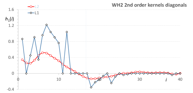
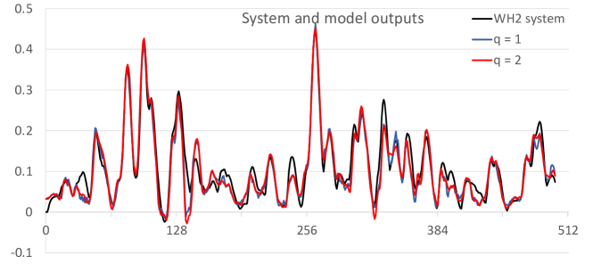
Comparing the diagrams in Figs. 5a,b one can observe that – in spite of various shapes of the kernels obtained for various $q$ – the WHB system models produced almost the same output signals. In attempt to replicate this phenomenon for the WH2 system we correlated its input signal by the dynamics $G\left(z\right)$ and removed the output noise; see Figs. 7a,b. Now, to explain this behavior, we denote by $\mathbf{\hat{\theta}}_{1}$, $\mathbf{\hat{\theta}}_{2}$ the solutions found by the algorithm for $q=1$ and for $q=2$, and by $\mathbf{S}$ the matrix composed from the consecutive Volterra terms

$$\mathbf{S} = [\mathbf{s}_{1}^{T},\mathbf{s}_{2}^{T},\allowbreak\dots,\allowbreak\mathbf{s}_{N}^{T}]^{T},$$

$$\mathbf{s}_{n} = [m_{1}\left(\mathbf{u}_{n}\right),\allowbreak m_{2}\left(\mathbf{u}_{n}\right),\allowbreak\dots,\allowbreak m_{D}\left(\mathbf{u}_{n}\right)]^{T},$$ (13)

The different shapes of the kernels, together with virtually the same outputs produced by either model, mean therefore that $\mathbf{S}\left(\mathbf{\hat{\theta}}_{1}-\mathbf{\hat{\theta}}_{2}\right)\approx\mathbf{0}$, which implies that the input signal correlation made the columns of $\mathbf{S}$ linearly dependent (i.e. the difference vector $\mathbf{\hat{\theta}}_{1}-\mathbf{\hat{\theta}}_{2}$ belongs to the null space of that matrix); cf. also [34], where the LASSO algorithm was tested for correlated data.

(a) Model errors (averaged over SNR = 1, 10, 40, 80 and 100).

(b) Model sparsities; $D$ = 861, SNR = 40, $N$ = 1000.

Figure 8: WH2 system. Comparison of model errors and their sparsities.

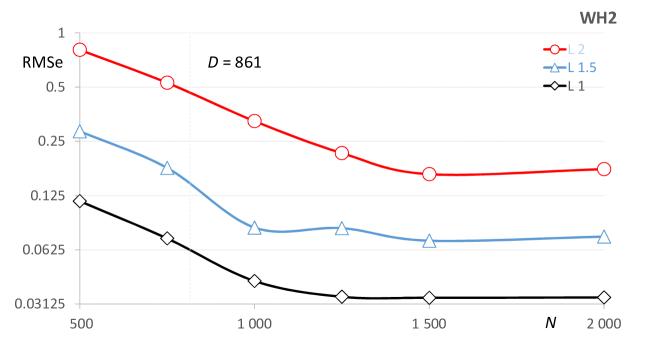
The performance of the proposed algorithms was finally compared to the algorithms based on Volterra series and unconstrained least squares approach. The results are presented in Fig. 9. One can observe that the models obtained by the proposed constrained algorithms (especially for $q=1$) have smaller error even when the number of measurements is significantly smaller ($N=500$ vs. $N=5000$) that in the unconstrained case. Comparing our results to those in the literature, we would like to point out that:

1. In the [21], where the $l_{1}$ algorithm was originally proposed, the error of the model was compared to the best possible model (that is, to the best approximation of the system by the Volterra series). The difference was apparently small; see Fig. 2 in [21]. We would also like to point out that the experiments made in [14] & [6] were based on systems with a relatively short memory so that the resulting models with $L=11$ and $P=3$ were of size $D=364$. In our benchmark experiment, in turn, the model with $D=2441$ (i.e. of order of magnitude larger) was used.

2. In the [30], where the $l_{1}$ algorithm was tested against the infinite memory nonlinear system, the comparison, similar to the added to the corrected version of the manuscript, was presented. The modeled system was again much simpler than the Wiener-Hammerstein benchmark examined in our manuscript and the resulting Volterra models were subsequently significantly smaller in size. Nevertheless, the advantage of the $l_{1}$ algorithm over the $LS$ ones is also noticeable there; see Fig. 3 in [30].

   

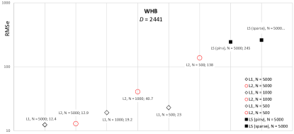
   Figure 9: Performance of the proposed constrained algorithms versus the unconstrained ones

V Conclusions

The problem of effective modeling of nonlinear dynamic systems using short data records remains both interesting from the formal viewpoint and important in practice. In the paper we examined the modeling algorithm based on Volterra series and convex optimization, and concluded that:

• The error between the resulting empirical models and their best possible theoretical counterparts is no larger than $\mathcal{O}(\sqrt{\ln D}/\sqrt{N})$ for any finite $D>2$. This makes the algorithm robust against overparametrization and superior to the unconstrained least squares algorithms, especially for $D\approx\sqrt{N}$; and, a fortiori, for $D\geq N$.

• The benchmark experiments confirmed such robustness for $q=1$ in particular and, to less extent, also for $q>1$. For $q=1$, the algorithm prefers sparse (“non-smooth”) solutions at the expense of its system nature modeling capability. On the other hand, the models obtained for $q=1.5,2$, while worse in terms of model error, are more accurate in reproducing the nature of the system.

The most apparent and challenging issue of the proposed approach is the large size of the Volterra models. This is however the consequence of a poor prior knowledge about the system structure and the variety of possible nonlinear structures and characteristics. It should be noted that if more prior knowledge is available then the more effective and parsimonious algorithms can be applied, however, such algorithms are specifically designed for particular system structures (be it Hammerstein, or Wiener, or Wiener-Hammerstein systems) and fail if the actual system is different than assumed; see e.g. [31, 32].

Proof of Theorem 7

The following derivation is based on the proof in [19] and extends the one in [21] for the case when $q>1$ by employing the norm inequality in (7). We use the matrix/vector notation

$$\mathbf{A}=E\left\{\mathbf{s}_{i}\mathbf{s}_{i}^{T}\right\},\mathbf{b}=2E\left\{\mathbf{s}_{i}y_{i}\right\},\text{ and }c=E\left\{y_{i}^{2}\right\},$$

where the vectors $\mathbf{s}_{i}$, $i=\tau+1,\ldots,N,$ are defined as in (13), so that $Q\left(\mathbf{\theta}\right)$ in (9) can be rewritten into a form

$$Q\left(\mathbf{\theta}\right)=\mathbf{\theta}^{T}\mathbf{A\theta}-\mathbf{\theta}^{T}\mathbf{b}+c=Q_{0}\left(\mathbf{\theta}\right)+c.$$

where $Q_{0}\left(\mathbf{\theta}\right)=\mathbf{\theta}^{T}\mathbf{A\theta}-\mathbf{\theta}^{T}\mathbf{b}$. Analogously, we define

$$\mathbf{\hat{A}}=\frac{1}{N-\tau}\sum_{i=\tau+1}^{N}\mathbf{s}_{i}\mathbf{s}_{i}^{T}.$$

Note that $\mathbf{\hat{A}}$, being an empirical counterpart of $\mathbf{A}$, is also a symmetric $D\times D$ matrix with the components

$$\mathbf{\hat{A}}_{lk}=\frac{1}{N-\tau}\sum_{i=\tau+1}^{N}m_{l}\left(\mathbf{u}_{i}\right)m_{k}\left(\mathbf{u}_{i}\right),$$

for $k,l=1,\ldots,D$. Defining similarly the other two vectors

$$\mathbf{\hat{b}}=\frac{2}{N-\tau}\sum_{i=\tau+1}^{N}\mathbf{s}_{i}y_{i}~{}\text{and }\hat{c}=\frac{1}{N-\tau}\sum_{i=\tau+1}^{N}y_{i}^{2}.$$

we get the following counterpart of (5)

$$\hat{Q}\left(\mathbf{\theta}\right)=\mathbf{\theta}^{T}\mathbf{\hat{A}\theta}-\mathbf{\theta}^{T}\mathbf{\hat{b}}+\hat{c}=\hat{Q}_{0}\left\{\mathbf{\theta}\right\}+\hat{c},$$

where

$$\hat{Q}_{0}\left(\mathbf{\theta}\right)=\mathbf{\theta}^{T}\mathbf{\hat{A}\theta}-\mathbf{\theta}^{T}\mathbf{\hat{b}.}$$

To show the bound for $E\{Q(\mathbf{\hat{\theta}})\}-Q\left(\mathbf{\theta}^{\ast}\right)$, we will use the inequality

$$Q(\mathbf{\hat{\theta})}-Q\left(\mathbf{\theta}^{\ast}\right) = Q_{0}(\mathbf{\hat{\theta})}-Q_{0}\left(\mathbf{\theta}^{\ast}\right)$$

$$= \left[Q_{0}(\mathbf{\hat{\theta})}-\hat{Q}_{0}\left(\mathbf{\hat{\theta}}\right)\right]+\left[\hat{Q}_{0}\left(\mathbf{\hat{\theta}}\right)-Q_{0}\left(\mathbf{\theta}^{\ast}\right)\right]$$

$$\leq 2\sup_{\left\|\mathbf{\theta}\right\|_{q}\leq D^{1/q-1}}\left|\hat{Q}_{0}\left(\mathbf{\theta}\right)-Q_{0}\left(\mathbf{\theta}\right)\right|,$$

which allows us to get rid from the analysis the empirical parameter vector $\mathbf{\hat{\theta}}$, as it now remains on the left-hand side only. The term in the right-hand side of the above inequality can further be decomposed as

$$\hat{Q}_{0}\left(\mathbf{\theta}\right)-Q_{0}\left(\mathbf{\theta}\right) = \mathbf{\theta}^{T}\mathbf{\hat{A}\theta}-\mathbf{\theta}^{T}\mathbf{\hat{b}}-\left[\mathbf{\theta}^{T}\mathbf{A\theta}-\mathbf{\theta}^{T}\mathbf{b}\right]$$

$$= \mathbf{\theta}^{T}\left(\mathbf{\hat{A}}-\mathbf{A}\right)\mathbf{\theta}-\mathbf{\theta}^{T}\left(\mathbf{\hat{b}}-\mathbf{b}\right).$$

Taking now into account that the constraint $\left\|\mathbf{\theta}\right\|_{1}\leq 1$ holds by virtue of the assumption in (6) and because of the norm inequality in (7), and by applying both triangle and Hölder inequalities to $\left|\mathbf{\theta}^{T}\left(\mathbf{\hat{A}}-\mathbf{A}\right)\mathbf{\theta}\right|\$and to $\left|\mathbf{\theta}^{T}\left(\mathbf{\hat{b}}-\mathbf{b}\right)\right|$, we get that

$$\left|\hat{Q}_{0}\left(\mathbf{\theta}\right)-Q_{0}\left(\mathbf{\theta}\right)\right|\leq 2\left\|\mathbf{\gamma}\right\|_{\infty},$$

where

$$\left\|\mathbf{\gamma}\right\|_{\infty}=\max_{i}\left|\mathbf{\gamma}_{i}\right|,\mathbf{\gamma}=[a_{11},\dots,a_{lk},b_{1},\dots,b_{D}]^{T},$$

is an auxiliary vector composed of the unique components $\left\{a_{lk}\right\},$ $1\leq l\leq k\leq D,$ of the matrix $\mathbf{\hat{A}}-\mathbf{A}$ and of components $\left\{b_{l}\right\}$ of the vector $\mathbf{\hat{b}}-\mathbf{b}$, respectively. Observing now that $\mathbf{\gamma}$ can be further rewritten as

$$\mathbf{\gamma=}\frac{1}{N-\tau}\sum_{i=\tau+1}^{N}\mathbf{\eta}_{i},$$

where

$$\mathbf{\eta}_{i}=[p_{11}\left(\mathbf{u}_{i}\right)\text{,}\dots\text{,}p_{lk}\left(\mathbf{u}_{i}\right)\text{,}\dots\text{,}p_{DD}\left(\mathbf{u}_{i}\right)\text{,}q_{1}\left(\mathbf{u}_{i}\right)\text{,}\dots\text{,}q_{D}\left(\mathbf{u}_{i}\right)]^{T}$$

for $1\leq l\leq k\leq D$, with

$$\begin{array}[]{l}p_{lk}\left(\mathbf{u}_{i}\right)=m_{l}\left(\mathbf{u}_{i}\right)m_{k}\left(\mathbf{u}_{i}\right)-E\left\{m_{l}\left(\mathbf{u}_{0}\right)m_{k}\left(\mathbf{u}_{0}\right)\right\},\\ q_{l}\left(\mathbf{u}_{i}\right)=2m_{l}\left(\mathbf{u}_{i}\right)\left[m\left(\mathbf{u}_{i}\right)+e_{i}\right]-2E\left\{m_{l}\left(\mathbf{u}_{0}\right)m\left(\mathbf{u}_{i}\right)\right\},\end{array}$$

we get the bound

$$E\{Q(\mathbf{\hat{\theta})\}}-Q\left(\mathbf{\theta}^{\mathbf{\ast}}\right) \leq 2E\left\{\sup_{\left\|\mathbf{\theta}\right\|_{1}\leq 1}\left|\hat{Q}_{0}\left(\mathbf{\theta}\right)-Q_{0}\left(\mathbf{\theta}\right)\right|\right\}$$

$$\leq \frac{4}{N-\tau}E\left\|\sum_{i=\tau+1}^{N}\mathbf{\eta}_{i}\right\|_{\infty}.$$

Recall now that the map $m\left(\cdot\right)$ and the dictionary elements are bounded by $M=\max\left\{M_{m},M_{d}\right\}$ (cf. Assumption A3), and hence

$$\left|p_{lk}\right|\left.\leq\right.2M^{2}\text{ and }\left|q_{l}\right|\leq 2M\left|e_{i}\right|+4M^{2},$$ (14)

for all $1\leq l\leq k\leq D$ and $i=\tau+1,\ldots,N$. Following from this point the proof as in [21], we will eventually get the bound

$$E\{Q(\mathbf{\hat{\theta}})\}-Q\left(\mathbf{\theta}^{\ast}\right)\leq C\frac{\sqrt{N}}{N-\tau}\sqrt{\left(\tau+1\right)\ln D},$$

with the constant $C=32\sqrt{e}\left(M\sigma+M^{2}\right)$, as in (10).

Remark 11.

To take into account the multiplication factor $R$, introduced in Algorithm III-B3, and to get the constant $C$ as in (11), we only need to replace the bounds in (14) by the following ones

$$\left|p_{lk}\right|\left.\leq\right.2\left(MR\right)^{2}\text{ and }\left|q_{l}\right|\leq 2MR\left|e_{i}\right|+4(MR)^{2},$$ (15)

for all $1\leq l\leq k\leq D$ and $i=\tau+1,\ldots,N$.

References

- [1] Ljung, L.: ‘Perspectives on system identification’, Annual Reviews in Control, 2010, 34, (1), pp. 1–12
- [2] Alper, P.: ‘A consideration of the discrete Volterra series’, Automatic Control, IEEE Transactions on, 1965, 10, (3), pp. 322–327
- [3] Boyd, S., Chua, L.O., Desoer, C.A.: ‘Analytical foundations of Volterra series’, IMA Journal of Mathematical Control and Information, 1984, 1, (3), pp. 243–282
- [4] Sanderg, I.W.: ‘Uniform approximation with doubly finite Volterra series’, Signal Processing, IEEE Transactions on, 1992, 40, (6), pp. 1438–1442
- [5] Pearson, R., Ogunnaike, B.A.: ‘Identification and control using Volterra models’. (Springer, 2002)
- [6] Kekatos, V., Giannakis, G.B.: ‘Sparse Volterra and polynomial regression models: Recoverability and estimation’, Signal Processing, IEEE Transactions on, 2011, 59, (12), pp. 5907–5920
- [7] Schoukens, M., Marconato, A., Pintelon, R., Vandersteen, G., Rolain, Y.: ‘Parametric identification of parallel Wiener–Hammerstein systems’, Automatica, 2015, 51, pp. 111–122
- [8] V. Z. Marmarelis, Nonlinear Dynamic Modeling of Physiological Systems, ser. IEEE Press Series on Biomedical Engineering. Piscataway, NJ: Wiley-IEEE Press, 2004.
- [9] F. J. Doyle III, R. K. Pearson, and B. A. Ogunnaike, Identification and Control Using Volterra Models. London: Springer-Verlag, 2002.
- [10] Cheng, C., Peng, Z., Zhang, W., Meng, G.: ‘Volterra-series-based nonlinear system modeling and its engineering applications: A state-of-the-art review’, Mechanical Systems and Signal Processing, 2017, 87, pp. 340–364
- [11] Wahlberg, B.: ‘System identification using laguerre models’, Automatic Control, IEEE Transactions on, 1991, 36, (5), pp. 551–562
- [12] Juditsky, A., Hjalmarsson, H., Benveniste, A., Delyon, B., Ljung, L., Sjoberg, J., et al.: ‘Nonlinear black-box models in system-identification - mathematical foundations’, Automatica, 1995, 31, (12), pp. 1725–1750
- [13] Vandersteen, G., Schoukens, J.: ‘Measurement and identification of nonlinear systems consisting of linear dynamic blocks and one static nonlinearity’, Automatic Control, IEEE Transactions on, 1999, 44, (6), pp. 1266–1271
- [14] Westwick, D.T., Kearney, R.E.: ‘Identification of Nonlinear Physiological Systems’. IEEE Press Series on Biomedical Engineering. (Piscataway: Wiley-IEEE Press, 2003)
- [15] Ogunfunmi, T.: ‘Adaptive nonlinear system identification: The Volterra and Wiener model approaches’. (Springer, 2007)
- [16] Marmarelis, V.Z.: ‘Nonlinear Dynamic Modeling of Physiological Systems’. IEEE Press Series on Biomedical Engineering. (Piscataway, NJ: Wiley-IEEE Press, 2004)
- [17] Boyd, S., Vandenberghe, L.: ‘Convex optimization’. (Cambridge university press, 2004)
- [18] Kakade, S.M., Shalev-Shwartz, S., Tewari, A.: ‘Regularization techniques for learning with matrices’, The Journal of Machine Learning Research, 2012, 13, (1), pp. 1865–1890
- [19] Juditsky, A., Nemirovski, A.: ‘Functional aggregation for nonparametric regression’, The Annals of Statistics, 2000, 28, (3), pp. 681–712
- [20] Nemirovski, A. ‘Topics in non-parametric statistics’. In: Bernard, P., editor. Lecture notes in Mathematics. vol. 1738. (New York: Springer, 2000.
- [21] Wachel, P., Śliwiński, P.: ‘Aggregative modelling of nonlinear systems’, IEEE Signal Processing Letters, 2015, 22, (9), pp. 1482–1486
- [22] Wang, Z., Liu, X., Liu, Y., Liang, J., Vinciotti, V.: ‘An extended Kalman filtering approach to modeling nonlinear dynamic gene regulatory networks via short gene expression time series’, IEEE/ACM Transactions on Computational Biology and Bioinformatics (TCBB), 2009, 6, (3), pp. 410–419
- [23] Zeng, N., Wang, Z., Li, Y., Du, M., Cao, J., Liu, X.: ‘Time series modeling of nano-gold immunochromatographic assay via expectation maximization algorithm’, IEEE Transactions on Biomedical Engineering, 2013, 60, (12), pp. 3418–3424
- [24] Schoukens, J., Suykens, J.A.K., Ljung, L. ‘Wiener-Hammerstein benchmark’. In: 15th IFAC Symposium on System Identification. (Saint-Malo, France, 2009.
- [25] Kibangou, A.Y., Favier, G.: ‘Wiener-Hammerstein systems modeling using diagonal Volterra kernels coefficients’, IEEE Signal Processing Letters, 2006, 13, (6), pp. 381
- [26] Tibshirani, R.: ‘Regression shrinkage and selection via the Lasso’, Journal of the Royal Statistical Society Series B (Methodological), 1996, pp. 267–288
- [27] Kukreja, S.L.: ‘Application of a least absolute shrinkage and selection operator to aeroelastic flight test data’, International Journal of Control, 2009, 82, (12), pp. 2284–2292
- [28] James, G., Witten, D., Hastie, T., Tibshirani, R.: ‘An introduction to statistical learning’. vol. 112. (Springer, 2013)
- [29] Boyd, S., Chua, L.: ‘Fading memory and the problem of approximating nonlinear operators with Volterra series’, Circuits and Systems, IEEE Transactions on, 1985, 32, (11), pp. 1150–1161
- [30] Wachel, P.: ‘Convex aggregative modelling of infinite memory nonlinear systems’, International Journal of Control, 2016, 89, (8), pp. 1613–1621
- [31] Wills, A., Ninness, B.: ‘Generalised Hammerstein–Wiener system estimation and a benchmark application’, Control Engineering Practice, 2012, 20, (11), pp. 1097–1108
- [32] Wachel, P., Mzyk, G.: ‘Direct identification of the linear block in Wiener system’, International Journal of Adaptive Control and Signal Processing, 2016, 30, (1), pp. 93–105
- [33] Marconato, A., Sjöberg, J., Schoukens, J.: ‘Initialization of nonlinear state-space models applied to the Wiener–Hammerstein benchmark’, Control Engineering Practice, 2012, 20, (11), pp. 1126–1132
- [34] Hebiri, M., Lederer, J.: ‘How correlations influence Lasso prediction’, Information Theory, IEEE Transactions on, 2013, 59, (3), pp. 1846–1854