Limited Evaluation Cooperative Co-evolutionary Differential
Evolution for Large-scale Neuroevolution

Abstract.

Many real-world control and classification tasks involve a large number of features. When artificial neural networks (ANNs) are used for modeling these tasks, the network architectures tend to be large. Neuroevolution is an effective approach for optimizing ANNs; however, there are two bottlenecks that make their application challenging in case of high-dimensional networks using direct encoding. First, classic evolutionary algorithms tend not to scale well for searching large parameter spaces; second, the network evaluation over a large number of training instances is in general time-consuming. In this work, we propose an approach called the Limited Evaluation Cooperative Co-evolutionary Differential Evolution algorithm (LECCDE) to optimize high-dimensional ANNs.

The proposed method aims to optimize the pre-synaptic weights of each post-synaptic neuron in different subpopulations using a Cooperative Co-evolutionary Differential Evolution algorithm, and employs a limited evaluation scheme where fitness evaluation is performed on a relatively small number of training instances based on fitness inheritance. We test LECCDE on three datasets with various sizes, and our results show that cooperative co-evolution significantly improves the test error comparing to standard Differential Evolution, while the limited evaluation scheme facilitates a significant reduction in computing time.

1. Introduction

Scaling artificial neural networks (ANNs) up to solve large complex problems achieved a big success in various machine learning problems. The backpropagation and stochastic gradient descent algorithms are conventional methods for training ANNs (LeCun et al., 1998). An alternative approach, Neuroevolution (NE) (Floreano et al., 2008), employs evolutionary algorithms to optimize the topology and/or weights of the ANNs. The NE algorithms do not require the gradient information, and perform remarkably well in optimizing ANNs based on the direct interaction with their environment; specifically, in the cases where good decision instances are noisy or not known for supervised learning (Floreano et al., 2008; Whitley et al., 1993).

There are mainly two types of NE approaches: direct and indirect encoding (Floreano et al., 2008). Direct encoding aims to evolve the network parameters directly representing them within the genotype of the individuals; whereas, indirect encoding aims to evolve the specifications to define the developmental process of an ANN represented within the genotype. The indirect encoding methods can help improving the scalability of the evolutionary process for large networks, since they can reduce the parameter size. On the other hand, the NE with direct encoding presents a challenging opportunity for stimulating the research in large-scale optimization, but also contributes to understanding the evolutionary dynamics of ANNs by suggesting successful evolutionary strategies to evolve ANNs.

The task of evolving direct-encoded large networks is challenging due to 1) the scalability of the evolutionary methods to perform the optimization process efficiently on high-dimensional search spaces, and 2) the time requirement for evaluating the individuals on a large number of training instances. The Cooperative Co-evolution (CC) is an effective approach for optimizing large-scale problems (Potter and De Jong, 1994); and the Limited Evaluation (LE) is an advantageous method for reducing the number of instances of fitness evaluations (Morse and Stanley, 2016). In this work, we propose a Limited Evaluation Cooperative Co-evolutionary Differential Evolution (LECCDE) algorithm that employs the CC and LE approaches to perform accelerated evolution in optimizing high-dimensional ANNs with direct encoding.

With respect to the previous works, the work presented in this paper contributes as follows: 1) it considers the post-synaptic neurons as the building blocks of an ANN, and performs the subcomponent decomposition of the CC scheme by assigning the pre-synaptic weights of each post-synaptic neuron to a subpopulation; 2) it demonstrates the effectiveness of the CC in optimizing large-scale ANNs, and compares with the standard Differential Evolution (DE) optimization; 3) it shows that the LE scheme enhanced with the CC achieves better accuracy results than standard DE for evolving large networks, while reducing the time required for the fitness evaluation.

Three datasets were chosen to evaluate the performance of the proposed algorithm on supervised learning tasks. We used a fully connected feed forward ANNs with one hidden layer, with a total number of parameters in the order of thousands. We refer to these ANNs as “large-scale” in the sense of NE with direct encoding, and to distinguish them from the specialized networks used in Deep Learning (DL) approaches (LeCun et al., 2015).

The rest of the paper is organized as follows: in Section 2, we provide the background knowledge and a brief literature review on the topics of DE, CC, and NE; in Section 3, we discuss the proposed algorithm in detail; in Section 4, we present the experimental setup; in Section 5, we provide the numerical results; and finally, in Section 6, we discuss the conclusions.

2. Related Work

In this section, we provide a brief overview of the background and related work.

2.1. Differential Evolution

The DE algorithm is a powerful yet simple population-based search algorithm for continuous optimization (Storn and Price, 1997). A candidate solution set consists of $NP$ individuals represented as $D$-dimensional real-valued vectors $\boldsymbol{x_{i}}\in\mathbb{R}^{D}$ where integer $i\in[1,NP]$. An initial population of individuals is randomly sampled from the domain ranges of each dimension $x_{i,j}^{min}$ and $x_{i,j}^{max}$ where $x_{i,j}$ is the $j$th dimension of $i$th individual.

In each generation $g$, an individual $\boldsymbol{x_{i}^{g}},\forall i\in(1,2,\cdots,NP)$, called the target vector, is selected. The mutation and crossover operators are applied to generate a trial vector $\boldsymbol{u^{g}}$. The trial vector is evaluated, and replaced with the target vector by the selection operator, if the fitness value of the trial vector is greater than or equal to the target vector.

The mutation operator generates a mutant vector $\boldsymbol{v_{i}^{g}}$ by perturbing a randomly selected vector using the scaled differences of the other two randomly selected vectors. The magnitude of the perturbation is controlled by the parameter called scale factor $(F)$. This strategy is referred to as the “rand/1” strategy, and is provided by the following equation:

(1) $$\boldsymbol{v_{i}^{g}}=\boldsymbol{x_{r_{1}}^{g}}+F\cdot(\boldsymbol{x_{r_{2}}^{g}}-\boldsymbol{x_{r_{3}}^{g}})$$

where $r_{1},r_{2},\mbox{ and }r_{3}$ are mutually exclusive integers different from $i$, and selected randomly from the range of $[1,NP]$. There are various alternative mutation strategies proposed in the literature (Das et al., 2016; Neri and Tirronen, 2010).

The crossover operator recombines the target vector with the mutant vector, controlled by the parameter called crossover rate $(CR)$. The binomial (uniform) and exponential crossover operators are the two most commonly used crossover operators (Price et al., 2006). The binomial crossover operator is provided in Equation (2):

(2) $$u_{i,j}^{g}=\left\{\begin{array}[]{lr}v_{i,j}^{g},&\mbox{if }rand([0,1))\leq CR\mbox{ or }j=randi([1,D]);\\ x_{i,j}^{g},&\mbox{otherwise.}\end{array}\right.$$

where integer $j\in[1,D]$ refers to the $j$th dimension of the vectors, functions $rand()$ and $randi()$ uniformly samples real and integer values within the specified ranges respectively.

The selection operator performs a comparison of the fitness values of the target and trial vectors, and replaces the target vector with the trial vector in the next generation if a better fitness value is achieved by the trial vector. This is referred to as synchronous update, since the replacements are performed at the end of the generation when the process for all individuals is complete. The asynchronous version of the update is implemented by performing the replacement immediately within the same generation. The asynchronous update allows a newly replaced trial vector to be used by other individuals within the same generation.

The settings of the parameters in DE plays an influential role in the behavior of the algorithm for balancing the trade-off between the exploration and exploitation (Neri and Tirronen, 2010; Črepinšek et al., 2013). A recent survey by Karafotias et al. reviewed the approaches for parameter tuning and control in evolutionary algorithms (Karafotias et al., 2015). Neri and Tirronen surveyed the existing works in the literature and performed an empirical analysis of the strategies and parameters in DE; more recently, Das et al. reviewed the works in the literature on the self-adaptive parameter control in DE (Das et al., 2016).

2.2. Cooperative Co-evolution

While the dimensionality of a problem increases, the performance of the evolutionary algorithms tend to decrease (Mahdavi et al., 2015; Liu et al., 2001). The CC schemes were proposed for scaling evolutionary algorithms to higher dimensions using a divide-and-conquer strategy. In the CC, the subcomponents of a large-scale problem is decomposed and assigned to a number of subpopulations, that are evolved separately (Potter and De Jong, 1994). Cooperation in co-evolution arises during the fitness evaluation, where the subcomponents are merged together to assign a global fitness score to a candidate solution.

The three aspects that play a key role in CC are problem decomposition, subcomponent evolution, and subcomponent co-adaptation (Yang et al., 2008). The maximum number of subpopulations can be generated by splitting a $D$-dimensional problem into $D$ subgroups, assigning each subcomponent (dimension) to one subpopulation. Alternatively, the number of subcomponents in each subpopulation can be chosen arbitrarily to make the evolutionary optimization process manageable by reducing the dimensionality per subgroup. However, an arbitrary assignment of subcomponents may not be effective for solving non-separable problems. Ideally, the problem should be decomposed in a way that the interdependency between the subcomponents in different subpopulations should be minimized.

The existing knowledge about the problem domain can be beneficial in the problem decomposition process. If the interdependencies of the subcomponents are known, the problem can be decomposed based on this knowledge. This also relates to the separability property of the problem. If the problem is separable, then the problem can be decomposed into its separable subcomponents. If there is no/uncertain knowledge of the problem domain, then automated methods can be used to identify the interactions of the subcomponents (Sun et al., 2017; Omidvar et al., 2014).

The subcomponent evolution can be performed by using various kinds of evolutionary algorithms (Mahdavi et al., 2015), including the DE (Shi et al., 2005).

2.3. Neuroevolution

ANNs are computational models that are inspired by the central nervous system (De Castro, 2006). NE is a field that aims to optimize ANNs by using evolutionary computing methods (Floreano et al., 2008). The approaches suggested in NE can be grouped as direct and indirect encoding methods. One of the first examples of the direct encoding approaches evolved the connection weights of fixed topology networks by representing them within the genotype of the individual in the population (Whitley et al., 1990; Fogel et al., 1990).

Neuroevolution of Augmenting Topologies (NEAT) has been proposed to evolve both the topology and the weights of the networks starting from minimal networks and incrementally grow larger networks through the evolutionary process (Stanley and Miikkulainen, 2002). NEAT uses a global innovation counter to keep track of the history of changes, and to align the networks to generate more meaningful offspring as a result of the crossover operator.

Some of the works incorporate the CC scheme within Neuroevolution. The Symbiotic Adaptive Neuroevolution (SANE) evolves two separate populations, one for neurons and another for the network “blueprints”. The evolved network blueprints are used to determine which combinations of the neurons to use from the neuron population to generate a network (Moriarty, 1997). The Enforced SubPopulations (ESP) initiates a subpopulation for each neuron, and the genotype of these neurons encode the weights for incoming, outgoing and bias connections (Gomez, 2003); Cooperative Synapse Neuroevolution (CoSyNE) initiates a subpopulation for each connection (Gomez et al., 2008).

The indirect NE methods can help scaling evolutionary approaches for evolving large networks. Kitano (Kitano, 1990) suggested a grammatical graph encoding method, based on graph rewriting rules represented as individuals’ genotypes, to evolve the connectivity matrix of ANNs. Koutnik et al., proposed using lossy compression techniques to reduce the high-dimensional parameters of the networks by transforming their parameters to the frequency domain using transformation functions such as the Fourier Transform and the Discrete Cosine Transform. In this case the evolutionary process is performed on a few significant coefficients on the frequency domain (Koutnik et al., 2010). Gruau suggested a developmental method that evolves tree-structured programs to specify the instructions to grow ANNs based on cell division and differentiation(Gruau, 1994). Stanley et al., proposed a Hypercube-Based Encoding method that uses Compositional Pattern Producing Networks (CPPNs) to assign the connection weights between neurons as a function of their locations (Stanley et al., 2009; Stanley, 2007).

The ANN architectures used in DL are often engineered for certain tasks in computer vision and signal processing(LeCun et al., 2015). In this case the connection weights are typically trained using the backpropagation. On the other hand, there are hyper-parameters for specifying the architecture and learning algorithms that play a role in the performance of network; thus, deep NE approaches have been suggested for optimizing the hyper-parameters of the deep neural networks efficiently (Miikkulainen et al., 2017; Real et al., 2017). Some recent work focuses on scalable evolutionary approaches for optimizing the connection weights of the networks. Salimans et al., used Evolution Strategies (ES) to optimize the connection weights of the Convolutional Neural Networks (CNNs) for reinforcement learning in MuJoCo and Atari environments (Salimans et al., 2017). The CNNs are a specific type of large ANN topologies that are specifically designed for image processing/recognition tasks in DL. Zhang et al., compared the ES proposed by Salimans et al. with the stochastic gradient descent for training CNNs on a large handwritten digit dataset, MNIST, and showed that the ES can achieve the state-of-the-art accuracy results (Zhang et al., 2017).

Another scalability challenge for the NE is the fitness evaluation that can be computationally expensive, especially when there are large numbers of training instances to evaluate. Morse and Stanley proposed an approach called Limited Evaluation Evolutionary Algorithm (LEEA), inspired by the batch training in the stochastic gradient descent algorithm. The LEEA performs fitness evaluations over a small number of training instances (batches), and uses accumulated fitness values that are inherited from the parent generation to the offspring generation between batches (Morse and Stanley, 2016). We adopt the LEEA approach in our algorithm, and discuss the approach in more detail in Section 3.

3. The Proposed Algorithm

The implementation details of the LECCDE algorithm are given in Algorithm 1. The algorithm is composed of the CC and LE schemes to decompose a large-scale continuous optimization task, and speed up the fitness evaluation process.

1:procedure LECCDE($NP$, $F$, $CR$)

2:     Initialize $NP$ individuals in each subpopulation $P_{i},i\in(1,SP)$

3:     Initialize $Ft_{i,j}\leftarrow 0$ $\triangleright$ Fitness of the $j$th individual in the $i$th subpopulation

4:     for $c=1$ to $trial\times NP$ do

5:         Select a random individual $\boldsymbol{x_{i,{r_{j}}}}$ from each $P_{i}$ $\triangleright$ $r_{j}$ is a randomly generated integer index

6:         $\boldsymbol{X}\leftarrow\{\boldsymbol{x_{1,{r_{1}}}},\boldsymbol{x_{2,{r_{2}}}},\cdots,\boldsymbol{x_{{SP},{r_{SP}}}}\}$

7:         $Ft_{X}\leftarrow evaluate(\boldsymbol{X},b_{1})$ $\triangleright$ $b_{1}$ is the first batch

8:         $\forall\boldsymbol{x_{i}}\in\boldsymbol{X},Ft_{i,j}\leftarrow Ft_{i,j}+Ft_{X}$

9:     end for

10:     $\forall i\in(1,SP)\mbox{ and }j\in(1,NP),Ft_{i,j}\leftarrow normalize(Ft_{i,j})$

11:     $\boldsymbol{X}\leftarrow\{\boldsymbol{x_{1,max}},\boldsymbol{x_{2,max}},\cdots,\boldsymbol{x_{SP,max}}\}$

12:     $Ft_{validation}\leftarrow evaluate(\boldsymbol{X},ValidationSet)$

13:     $bestValidation\leftarrow Ft_{validation}$

14:     $bestNetwork\leftarrow\boldsymbol{X}$

15:     while termination criterion is not satisfied do

16:         for each $b_{k}\in Batches$ do

17:              for each subpopulation $P_{i}$ do

18:                  $P_{i}^{\prime}\leftarrow P_{i}$

19:                  $Ft_{i}^{\prime}\leftarrow Ft_{i}$

20:                  for each $\boldsymbol{x_{i,j}}\in P_{i}$ do

21:                       $\boldsymbol{X_{i}}\leftarrow\boldsymbol{x_{i,j}}$

22:                       $Ft_{X}\leftarrow evaluate(\boldsymbol{X},b_{k})$

23:                       $Ft_{X}^{\prime}\leftarrow Ft_{i,j}\cdot(1-decay)+Ft_{X}$

24:                       $\boldsymbol{v}\leftarrow mutate(\boldsymbol{x_{i,r_{1}}},\boldsymbol{x_{i,r_{2}}},\boldsymbol{x_{i,r_{3}}},F)$

25:                       $Ft_{v}\leftarrow(Ft_{i,r_{1}}+Ft_{i,r_{2}}+Ft_{i,r_{3}})\diagup 3$

26:                       $\boldsymbol{u}\leftarrow crossover(\boldsymbol{x_{i,j}},\boldsymbol{v},CR)$

27:                       $\boldsymbol{X_{i}}\leftarrow\boldsymbol{u}$

28:                       $Ft_{u}\leftarrow evaluate(\boldsymbol{X},b_{k})$

29:                       $Ft_{u}^{\prime}\leftarrow((Ft_{i,j}+Ft_{v})\diagup 2)\cdot(1-decay)+Ft_{u}$

30:                       if $Ft_{u}^{\prime}>Ft_{X}^{\prime}$ then

31:                           $P_{i,j}^{\prime}\leftarrow\boldsymbol{u}$

32:                           $Ft_{i,j}^{\prime}\leftarrow Ft_{u}^{\prime}$

33:                       else

34:                           $P_{i,j}^{\prime}\leftarrow\boldsymbol{x_{i,j}}$

35:                           $Ft_{i,j}^{\prime}\leftarrow Ft_{X}^{\prime}$

36:                       end if

37:                  end for

38:                  $P_{i}\leftarrow P_{i}^{\prime}$

39:                  $Ft_{i}\leftarrow Ft_{i}^{\prime}$

40:                  $\boldsymbol{X_{i}}\leftarrow\boldsymbol{x_{i,max}}$

41:                  $Ft_{validation}\leftarrow evaluate(\boldsymbol{X},ValidationSet)$

42:                  if $Ft_{validation}>bestValidation$ then

43:                       $bestNetwork\leftarrow X$

44:                       $bestValidation\leftarrow Ft_{validation}$

45:                  end if

46:              end for

47:         end for

48:     end while

49:end procedure

Algorithm 1 LECCDE

The CC scheme in LECCDE uses a heuristic to decompose the parameters of a high-dimensional ANN, i.e. the post-synaptic neurons are assumed to be the building blocks of the ANN, and are decomposed into subpopulations and evolved separately. Thus, the algorithm initiates $SP$ subpopulations for each post-synaptic neuron, where each subpopulation consists of $NP$ individuals. Each individual represents the pre-synaptic connection weights (see Appx. A).

From the $SP$ subpopulations that contain $NP$ of individuals, there are $NP^{SP}$ ANNs that can be constructed. To find the average fitness of each individual, all possible network combinations need to be evaluated. Since this number is quite large, we randomly sample $trial\times NP$ times an individual from each subpopulation, construct a global network, evaluate it, and add the fitness value of the network to the fitness values of each individual that was part of the network (Gomez et al., 2008). At the end of this procedure, the fitness value of each individual is normalized to find the average fitness value, dividing by the number of time each individual is selected. The fitness of the individuals that were not selected during the sampling process set to 0. The individual with the maximum fitness from each subpopulation is then selected to construct the global ANN solution $\boldsymbol{X}$. Finally, the performance of the global solution on the validation instances is found by evaluating $\boldsymbol{X}$ on the validation set.

The main loop of the algorithm iterates over all the batches. A batch is a small subset of the training instances used in the LE scheme (Morse and Stanley, 2016). In particular, $TrainingSize\diagup BatchSize$ batches are generated by randomly assigning each training instance to a batch.

The fitness score of the target vector on the current batch is found by replacing it within its corresponding part in the global solution, and evaluating the global solution on the current batch. Subsequently, the fitness of the target vector is adjusted using the asexual reproduction rule (see Appx. A.2).

The fitness of the trial vector is computed in a similar fashion, by first replacing its corresponding part within the global solution, and then evaluating the global solution on the current batch. Since the mutant vector is composed of three randomly selected individuals $\{\boldsymbol{x_{i,r_{1}}},\boldsymbol{x_{i,r_{2}}},\boldsymbol{x_{i,r_{3}}}\}$, the fitness value of the mutant vector is computed by taking their average. The fitness value of the trial vector is found using the sexual reproduction rule (see Appx. A.2).

The selection operator copies the trial vector and its fitness to a temporary set if its fitness value is greater than or equal to the fitness value of the target vector; otherwise, the target value and its fitness are copied. After all the computations are completed for all individuals in the subpopulation, the subpopulation is updated simultaneously by copying back the individuals and their fitnesses from the temporary sets.

After each subpopulation update, the individual with the highest fitness value in the subpopulation is copied back to the corresponding part of the global solution $\boldsymbol{X}$. The global solution is evaluated on the validation set, and the one that performed the best is stored and provided as a the final result of the algorithm.

4. Experimental setup

Our experimental setup is designed to focus on the following questions:

1. Do the ANNs that are evolved using the Cooperative Co-evolutionary DE algorithm with our subpopulation assignment heuristic achieve a better classification accuracy than the ANNs that are evolved by the standard DE algorithm?

2. Does the LE scheme applied to DE reduce the runtime of the algorithm, without decreasing the classification accuracy of the evolved ANNs?

To answer these questions, we compare the results of the ANNs optimized by four algorithms, DE, LEDE, CCDE, and LECCDE, on three datasets with various sizes. The details for the implementation of the LECCDE are given in Algorithm 1. The CCDE and LEDE are implemented in a similar way, but, without the batch loop and the subpopulations, respectively. In standard DE, both batch training and subpopulations are not used. The LE algorithms require two evaluation per generation (target and trial vectors are evaluated on the current batch), while the algorithms without LE require one evaluation per generation. Regardless of this fact, the algorithms were run for the same number of function evaluations (FEs) for each dataset. For all experiments, we used “rand/1/bin” (“rand/1” mutation with binomial crossover) strategy with empirically fixed the parameter settings of $F$ and $CR$ to $0.1$ and $0.3$, respectively. We used $20$ individuals for the population size, except for one experiment that we performed on a larger population size consisting of $100$ individuals (see below). We set $trial$ parameter to 5.

The three datasets used in the test process are listed in Table 1. These datasets were obtained from the Center for Machine Learning and Intelligent Systems dataset repository (Lichman, 2013). These datasets were chosen based on their number of features and instances, to show the relative performance of the algorithms in respect to the size of the dataset used. The Wisconsin breast cancer (WBC) dataset consists of 30 features, 2 classes, and 569 instances, the epileptic seizure recognition (ESR) consists of 178 features, 2 classes, and 4600 instances, and the human activity recognition (HAR) dataset consists of 561 features, 6 classes, and 7144 instances (Anguita et al., 2013). The instances in each dataset were split into three groups (training, validation, and test) with ratios $70\%$, $15\%$, and $15\%$ respectively. The fitness evaluations and selection process were performed on the train instances. The network that performs the best on the validation set is provided as the output of the algorithm, and evaluated on the test set. The fitness evaluation is based on the classification accuracy of the ANNs which is calculated by the number of correctly classified instances divided by the total number of instances.

For all datasets, we used fixed-topology fully-connected feed forward ANNs with one hidden layer to perform the classification task (see Appx. A). The number of neurons within the hidden layer was kept constant at $50$ for all ANNs evolved for all datasets. Based on the architecture of the ANNs and the number of features in the datasets, the total number of parameters evolved are 1652, 9052, and 28406 for the WBC, ESR, and HAR respectively.

We used a batch size of 100 instances for the WBC, 500 for the ESR, and 500 for the HAR. The decay value (see Appx. A.2) is set to 0.2, as suggested by Morse and Stanley (Morse and Stanley, 2016). The maximum number of FEs was set to 50000 for the WBC, 300000 for the ESR, and 500000 for the HAR, based on the number of their parameters.

Table 1. The specifications of the datasets used in the experiments.

Datasets	Features	Classes	Instances	Parameters
WBC	30	2	569	1652
ESR	178	2	4600	9052
HAR	561	6	7144	28406

5. Numerical results

In this section, we present our experimental results. Each algorithm, with the specified settings, was run for 20 independent runs, and the median and the variance of train, validation and test accuracy were collected. All the accuracy results are shown with a precision of two digits.

Table 2 shows the results obtained from the WBC dataset. In this case we could not observe a significant difference on the results of the ANNs evolved by the four algorithms. On the test data, the CCDE appears to be performing better than others. On the other hand, we observe a difference on the runtime of the algorithm ($t=322$ sec, in our computing environment). The algorithms that employ LE and CC are less computationally expensive and run faster. For example, the runtime of DE is more than twice as big as that of LECCDE. This difference is less significant for the other algorithms, due to the size of the dataset. Even though all the algorithms are run for 50000 FEs for this dataset, the algorithms with LE performed evaluation on batches that are four times smaller than the whole set of training instances. However, since CCDE is run on the whole dataset, it appears that the CC improved its runtime possibly due to the computations of reduced-sized vectors within each subpopulation.

Table 2. The median of the accuracy results of the ANNs evolved using four variants of DEs on the WBC dataset.

Alg.	Train	Validation	Test	Runtime
DE	94.74 $\pm$ 2.2	97.65 $\pm$ 0.8	95.29 $\pm$ 2.2	$2.12\times t$
LEDE	95.99 $\pm$ 1.2	98.82 $\pm$ 0.6	95.29 $\pm$ 2.3	$1.43\times t$
CCDE	96.49 $\pm$ 1.3	97.65 $\pm$ 0.8	96.47 $\pm$ 1.8	$1.10\times t$
LECCDE	96.24 $\pm$ 1.9	97.65 $\pm$ 0.8	95.29 $\pm$ 2.8	$t$

Table 3 presents the results obtained from the ESR dataset. Based on the test data, CCDE appears to show better performance than the rest of the algorithms, while LECCDE follows it very closely. We observe the best running time with LECCDE ($t=2970$ sec).

Table 3. The median of the accuracy results of the ANNs evolved using four variants of DEs on the ESR dataset.

Alg.	Train	Validation	Test	Runtime
DE	90.50 $\pm$ 1.3	89.86 $\pm$ 1.2	89.57 $\pm$ 1.7	$2.66\times t$
LEDE	92.86 $\pm$ 0.9	92.25 $\pm$ 0.8	91.30 $\pm$ 0.9	$1.26\times t$
CCDE	93.94 $\pm$ 0.8	93.33 $\pm$ 0.3	92.17 $\pm$ 0.9	$2.05\times t$
LECCDE	93.98 $\pm$ 0.6	92.61 $\pm$ 0.5	91.88 $\pm$ 1.0	$t$

Table 4 shows the results obtained from the HAR dataset. On this dataset, we observe a significant accuracy improvement when the CC scheme is used. The performance of CCDE and LECCDE are approximately %15-20 better than the algorithms that do not use the CC. Also, CCDE appears to be slightly better than LECCDE. On the other hand, we observe a significant runtime improvement when the LE scheme is used. The algorithms with the LE scheme run approximately four times faster than the algorithms that do not use the LE ($t=6530$ sec). Also, LECCDE appears to produce the smallest variance on th train accuracy.

Table 4. The median of the accuracy results of the ANNs evolved using four variants of DEs on the HAR dataset.

Alg.	Train	Validation	Test	Runtime
DE	70.06 $\pm$ 2.9	70.06 $\pm$ 2.7	68.38 $\pm$ 3.0	$4.75\times t$
LEDE	77.5 $\pm$ 5.2	77.99 $\pm$ 4.8	76.96 $\pm$ 4.8	$1.28\times t$
CCDE	94.01 $\pm$ 0.8	92.72 $\pm$ 0.7	92.4 $\pm$ 1.0	$4\times t$
LECCDE	93.58 $\pm$ 0.6	93.19 $\pm$ 0.5	92.16 $\pm$ 0.7	$t$

Finally, in Table 5, we report an additional experiment on the population size. In this case, we used a population size of 100 on the ESR dataset. When the population size increases (comparing to the Table 3), the accuracy results decrease. This may be due to the number of FEs needed for the convergence of the algorithm: in other words, when the population increases, the number of FEs needed for the convergence may increase. Moreover, we observe that CCDE and LECCDE perform significantly better than DE and LEDE. This may suggest that the CC increased the convergence speed. With respect to the running time of the algorithms, we observe the similar pattern observed in Table 3 ($t=2640$ sec).

Overall, CCDE appears to perform better than LECCDE due to the fact that it has the complete information for evaluating the individuals since it uses the entire set of training instances. However, CCDE comes with a larger runtime trade-off than LECCDE, which can make the difference with large datasets (e.g. for the HAR dataset the LECCDE runs on average four times faster). Also, increasing the number of evaluations or batch size can improve the performance of the LECCDE. For comparison, we performed two additional experiments with LECCDE, with the same settings used to produce the results in the Table 4, except the number of FEs and batch size. In the first experiment, we used 900000 FEs and observed that the ANNs the LECCDE optimize perform on training, validation and test sets on average 95.78, 94.31, and 93.28 respectively. This is almost %1 higher than the the performance observed in 4. On the other hand, the runtime of the algorithm is now $1.6\times t$, which is still $1.8$ times faster than the runtime of CCDE. In the second experiment, we used a batch size of 1000, and we observed that the algorithm performs on average 96.60, 93.84, and 93.38 on training, validation, and test datasets, with a runtime of $1.42\times t$. These two additional experiments show an interesting trade-off between the batch size and the number of evaluations. Although the two additional experiments have similar runtime, the second experiment appears to produce better results.

Table 5. The median of the accuracy results of the ANNs evolved using four variants of DEs on the ESR dataset using population size of 100.

Alg.	Train	Validation	Test	Runtime
DE	81.99 $\pm$ 1.4	82.61 $\pm$ 1.2	80.65 $\pm$ 1.9	$2.62\times t$
LEDE	80.25 $\pm$ 1.4	81.59 $\pm$ 0.8	80.14 $\pm$ 2.2	$1.30\times t$
CCDE	91.65 $\pm$ 1.3	91.45 $\pm$ 0.7	90.29 $\pm$ 0.9	$2.01\times t$
LECCDE	91.27 $\pm$ 0.8	90.58 $\pm$ 0.7	88.99 $\pm$ 1.1	$t$

Figure 1 shows the overall comparison of the runtime of LEDE, CCDE, and DE relative to LECCDE on the three datasets. The $x$-axis shows the dataset, and the $y$-axis shows the increase in the runtime of the algorithm. The LEDE is relatively stable across experimented datasets. On the other hand, the runtime of the CCDE and DE increases when the number of instances increases. This is because the algorithms with LE perform the same number of function evaluations, on a smaller number of instances, which produces a clear advantage in terms of total runtime.

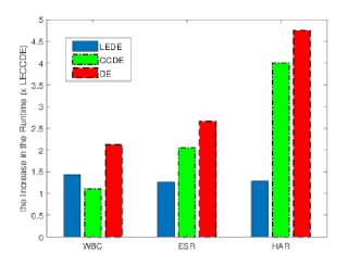
Figure 1. The increase in the runtime of each algorithm relative to the LECCDE on the three datasets.

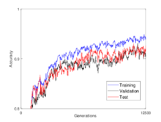
Figure 2. The change of the accuracy results of the ANNs on the training, validation, and test instances while the LECCDE algorithm is running.

Figure 2 shows the accuracy trend of the ANNs on the training, validation, and test instances during one example run of the optimization process performed by LECCDE (only the range $[0.8,1]$ is shown on the $y$-axis, for the sake of clarity). The data collected from this specific run shows that the accuracy on the training data is almost always the highest. The accuracy results of the test data closely follows the validation accuracy, and it is even higher for some of generations.

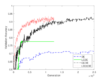
Figure 3. A single run of the change of the validation accuracy during the evolutionary process of four algorithms on the HAR dataset.

Figure 3 shows the change of the validation accuracy during the evolutionary process of four algorithms on a single run (only the range $[0.6-1]$ is shown on the $y$-axis). Firstly, the lines that represent the results of the LEDE and LECCDE are shorter than those of the other algorithms because they consume the same number of FEs within a half number of generations, since they perform two FEs (trial and target vectors) per generation. We observe that LEDE improves the DE in terms of validation accuracy and convergence speed; however, it suffers from the lack of diversity within the population (for a population size of 20), which prevents it from finding better solutions after about 80000 FEs are consumed. On the other hand, CCDE appears not to suffer from the early convergence problem observed in the LEDE, while LECCDE appears to improve the speed of CCDE.

To summarize, our empirical analysis suggests positive answers to the questions posed in Section 4: (1) It appears more significantly on large dataset (in Table 4), or with a large population size (in Table 5), that the ANNs that are evolved using the CC scheme using our heuristic achieve a better classification accuracy than the ANNs that are evolved by the standard DE algorithm; and (2) all experiments on the three datasets (most significantly on the largest dataset in Table 4), show that the LE scheme applied to DE reduce the runtime of the algorithm considerably, without causing a degradation on the classification accuracy of the evolved ANNs.

To further assess the scalability of the proposed algorithm, we performed an additional experiment on the MNIST dataset (LeCun et al., 1998). We used the same ANN architecture that was used in the previous experiments. We provide the numerical results —which are not shown here for brevity— on the extended version of the paper available online. For the same number of function evaluations, the computing time required for the LEDE and LECCDE is about 25 times less than the computing time required for the DE and CCDE. The LECCDE performs 8% better than LEDE. Overall, our preliminary results on MNIST show that the LECCDE achieves 90.80% classification accuracy on the test data, on average, which is about 4% lower than the backpropagation algorithm on the same ANN architecture. This may suggest that a better parameter tuning may be needed for the LECCDE to obtain results which are comparable to the state-of-the-art.

6. Conclusions

In this work, we proposed the LECCDE algorithm that employs the LE and CC schemes to improve the accuracy and the runtime of the standard DE algorithm for large-scale NE with direct encoding.

We performed experiments on four datasets, including a preliminary test on the MNIST dataset. Our results show that the CC scheme improves the performance of DE on the tested classification tasks. Moreover, we used the LE scheme to further improve the scalability of the method. Our results show that the LE scheme reduces the runtime of the algorithms, without affecting the performance. This reduction is due to the fact that the evaluation is performed on a small number of instances.

We used a heuristic in the CC scheme that decomposes the problem at the level of post-synaptic neurons. Thus, we evolve all the pre-synaptic weights of the post-synaptic neurons in different subpopulations. This decomposition approach aims to reduce the parameter size per subpopulation. For large datasets on the other hand, the number of parameters per subpopulation may still be large. Although this heuristic worked well, there may also be other decomposition heuristics that can be more effective. Alternatively, automatic methods can also be used for this purpose.

Another possibility for improving the results can be achieved by performing a sensitivity analysis. In this work, we did not experiment on the strategy and the parameters settings of the DE algorithm. Self-adaptive parameter control approaches can also be investigated to improve the performance of the results since these approaches can adjust the balance between the exploration and exploitation during the search process (Yaman et al., 2018; Das et al., 2016).

The methods proposed here can evolve only the ANNs with fixed topologies, it will be useful to extend these methods also to the network topology optimization.

Appendix A Neuroevolution

A.1. Direct Encoding and Network Computation

An example of a feed forward network (FFN) is shown in Figure 4a where each node represents a neuron, and each edge represents a connection between two node, and the direction of each edge represents the direction of the information flow. A FFN consists of a number of input ($i_{1},i_{2},i_{3},b_{1}$), hidden ($h_{1},h_{2},b_{2}$), and output ($o_{1}$) neurons ($b_{1}$ and $b_{2}$ are bias neurons kept constant at 1) structured as input, hidden and output layers respectively (see Figure 4a). Inspired by biological neural networks, the connections between the neurons are often called synapses. A neuron that is at the starting point of the directional edge is called a pre-synaptic neuron, and the neuron that is at the end point (arrow) of the directional edge is called a post-synaptic neuron.

(a)

post-synaptic neurons: $h_{1}$ $h_{2}$ $o_{1}$ pre-synaptic weights: 0.7 0.8 0.1 0.4 2.1 0.6 1.2 1.4 0.3 0.5 1.3 (b)

Figure 4. LABEL:sub@fig:FFN A fully-connected feed-forward ANN with one hidden layer, and LABEL:sub@tab:FFNGenotype the representation of its genotype.

Figure 4b shows the genotype representation of the network given in Figure 4a. Each synaptic weight is mapped directly to a gene in the genotype. The genotype is divided into its subcomponents consisting of the pre-synaptic weights of each post-synaptic neuron.

The activation of each neuron is updated using Equation (3) where $a_{i}$ is the activation of a post-synaptic neuron, $a_{j}$ is the activation of the $j$th pre-synaptic neuron and $w_{i,j}$ is the connection between them, $b_{i}$ is the bias of the post-synaptic neuron, and $\psi$ is an activation function given in (4) (De Castro, 2006).

(3) $$a_{i}=\psi\left(\sum_{j}w_{i,j}\cdot a_{j}+b_{i}\right)$$

(4) $$\psi(x)=\frac{2}{1+e^{-2x}}-1$$

A.2. Limited Evaluation

When the evaluation is performed episodically on a small subset of the whole training instances (batches), it is required to keep track of the individuals that performed well on the previous episodes. The LE scheme aims to adjust the fitness of the offspring by taking into account the success of its parents by fitness inheritance. The sexual and asexual reproduction rules are provided in Equations (5) and (6) respectively (Morse and Stanley, 2016).

(5) $$f^{\prime}=f_{parent}\cdot(1-decay)+f$$

(6) $$f^{\prime}=\frac{f_{parent_{1}}+f_{parent_{2}}}{2}\cdot(1-decay)+f$$

where, $f^{\prime}$ is the adjusted fitness of the offspring, $f_{parent}$ is the parent of its parent, $f$ is the actual fitness of the offspring on current batch of the training instances, and $decay$ is a constant value for adjusting the weight of the previous fitness evaluations. The sexual reproduction method consists of two parents.

Appendix B Extended experiments and results

This section presents our preliminary results of the experiments performed on the MNIST dataset using the DE, LEDE, CCDE and LECCDE. The MNIST dataset consists of 60000 samples of 28 by 28 grayscale image instances of handwritten numbers between 0-9. Thus, the size of the input and output are 784 and 10 when each image pixel and its class label are considered as an input and output respectively.

We used the same architecture of the artificial neural networks that were used for the experiments performed on the other datasets (feed forward artificial neural networks with one hidden layer consisting of 50 neurons). Thus, the total number of parameters of the networks optimized for the MNIST is 47710. The parameters of the Differential Evolution algorithm are also initialized using the same settings used for the other experiments except for batch size, number of individuals in each subpopulation and the maximum number of function evaluations. Since MNIST is larger than the tested other datasets, we used a a batch size of 1000, a population size of 60 and a maximum number of evaluations set to $2.16e+6$.

Table 6 shows the training, validation and test accuracy results of the ANNs trained for the MNIST dataset. Each variant of the algorithm was executed for the same number of function evaluations. The total time required for computing every other algorithm is shown in relation to the computing time required for the LECCDE where $t=6.6e+5$ seconds that is approximately 19 hours on a single-core Intel Xeon E5 3.5GHz computer. Due to time constraints, we were able to perform 3 independent runs for the LEDE and LECCDE, and a single partial run for the DE and CCDE. Thus, on DE and CCDE we report their accuracy at 12% of their total allocated computing time (the total computing times of DE and CCDE are estimated based on their current execution progress).

Table 6. The accuracy the ANNs evolved for the MNIST dataset, and the runtime of the algorithms.

Alg.	Train	Validation	Test	Runtime
DE (% 12)	61.60	61.26	62.52	$27.2\times t$
LEDE	82.68 $\pm$ 0.36	82.01 $\pm$ 0.75	82.23 $\pm 0.25$	$1.1\times t$
CCDE (% 12)	62.40	61.80	63.20	$25.3\times t$
LECCDE	91.79 $\pm$ 0.28	91.01 $\pm$ 0.63	90.80 $\pm$ 0.15	$t$

We observe a significant advantage in using the LE scheme on MNIST from the computing time point of view: indeed, the DE and CCDE implementations of the algorithm require a computing time that is 25 times bigger than the computing time required by the corresponding algorithms that make use of the LE scheme.

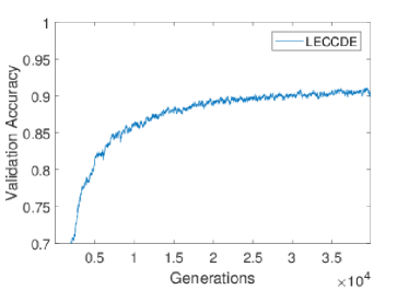
Figure 5. The change of the validation accuracy of the ANNs evolved using the LECCDE on MNIST dataset (only $[0.7,1]$ range is shown on the $y$-axis).

Figure 5 illustrates the change of the validation accuracy of the evolved ANNs using the LECCDE during an evolutionary process. The speed of the accuracy improvements slows down around 88% - 90% level. The best validation accuracy achieved during this evolutionary run was 91.62%.

References

- (1)
- Andrzejak et al. (2001) Ralph G Andrzejak, Klaus Lehnertz, Florian Mormann, Christoph Rieke, Peter David, and Christian E Elger. 2001. Indications of nonlinear deterministic and finite-dimensional structures in time series of brain electrical activity: Dependence on recording region and brain state. Physical Review E 64, 6 (2001), 061907.
- Anguita et al. (2013) Davide Anguita, Alessandro Ghio, Luca Oneto, Xavier Parra, and Jorge Luis Reyes-Ortiz. 2013. A Public Domain Dataset for Human Activity Recognition using Smartphones.. In ESANN.
- Črepinšek et al. (2013) Matej Črepinšek, Shih-Hsi Liu, and Marjan Mernik. 2013. Exploration and exploitation in evolutionary algorithms: A survey. ACM Computing Surveys (CSUR) 45, 3 (2013), 35.
- Das et al. (2016) Swagatam Das, Sankha Subhra Mullick, and Ponnuthurai N Suganthan. 2016. Recent advances in differential evolution–an updated survey. Swarm and Evolutionary Computation 27 (2016), 1–30.
- De Castro (2006) Leandro Nunes De Castro. 2006. Fundamentals of natural computing: basic concepts, algorithms, and applications. CRC Press.
- Floreano et al. (2008) Dario Floreano, Peter Dürr, and Claudio Mattiussi. 2008. Neuroevolution: from architectures to learning. Evolutionary Intelligence 1, 1 (2008), 47–62.
- Fogel et al. (1990) David B Fogel, Lawrence J Fogel, and VW Porto. 1990. Evolving neural networks. Biological cybernetics 63, 6 (1990), 487–493.
- Gomez et al. (2008) Faustino Gomez, Jürgen Schmidhuber, and Risto Miikkulainen. 2008. Accelerated neural evolution through cooperatively coevolved synapses. Journal of Machine Learning Research 9, May (2008), 937–965.
- Gomez (2003) Faustino John Gomez. 2003. Robust non-linear control through neuroevolution. Ph.D. Dissertation. University of Texas at Austin USA.
- Gruau (1994) Frédéric Gruau. 1994. Automatic definition of modular neural networks. Adaptive behavior 3, 2 (1994), 151–183.
- Karafotias et al. (2015) Giorgos Karafotias, Mark Hoogendoorn, and Ágoston E Eiben. 2015. Parameter control in evolutionary algorithms: Trends and challenges. IEEE Transactions on Evolutionary Computation 19, 2 (2015), 167–187.
- Kitano (1990) Hiroaki Kitano. 1990. Designing neural networks using genetic algorithms with graph generation system. Complex systems 4, 4 (1990), 461–476.
- Koutnik et al. (2010) Jan Koutnik, Faustino Gomez, and Jürgen Schmidhuber. 2010. Evolving neural networks in compressed weight space. In Proceedings of the 12th annual conference on Genetic and evolutionary computation. ACM, 619–626.
- LeCun et al. (2015) Yann LeCun, Yoshua Bengio, and Geoffrey Hinton. 2015. Deep learning. nature 521, 7553 (2015), 436.
- LeCun et al. (1998) Yann LeCun, Léon Bottou, Yoshua Bengio, and Patrick Haffner. 1998. Gradient-based learning applied to document recognition. Proc. IEEE 86, 11 (1998), 2278–2324.
- Lichman (2013) M. Lichman. 2013. UCI Machine Learning Repository. (2013). http://archive.ics.uci.edu/ml
- Liu et al. (2001) Yong Liu, Xin Yao, Qiangfu Zhao, and Tetsuya Higuchi. 2001. Scaling up fast evolutionary programming with cooperative coevolution. In Evolutionary Computation, 2001. Proceedings of the 2001 Congress on, Vol. 2. Ieee, 1101–1108.
- Mahdavi et al. (2015) Sedigheh Mahdavi, Mohammad Ebrahim Shiri, and Shahryar Rahnamayan. 2015. Metaheuristics in large-scale global continues optimization: A survey. Information Sciences 295 (2015), 407–428.
- Miikkulainen et al. (2017) Risto Miikkulainen, Jason Liang, Elliot Meyerson, Aditya Rawal, Dan Fink, Olivier Francon, Bala Raju, Arshak Navruzyan, Nigel Duffy, and Babak Hodjat. 2017. Evolving deep neural networks. arXiv preprint arXiv:1703.00548 (2017).
- Moriarty (1997) David Eric Moriarty. 1997. Symbiotic evolution of neural networks in sequential decision tasks. Ph.D. Dissertation. University of Texas at Austin USA.
- Morse and Stanley (2016) Gregory Morse and Kenneth O Stanley. 2016. Simple evolutionary optimization can rival stochastic gradient descent in neural networks. In Proceedings of the Genetic and Evolutionary Computation Conference 2016. ACM, 477–484.
- Neri and Tirronen (2010) Ferrante Neri and Ville Tirronen. 2010. Recent advances in differential evolution: a survey and experimental analysis. Artificial Intelligence Review 33, 1-2 (2010), 61–106.
- Omidvar et al. (2014) Mohammad Nabi Omidvar, Xiaodong Li, Yi Mei, and Xin Yao. 2014. Cooperative co-evolution with differential grouping for large scale optimization. IEEE Transactions on evolutionary computation 18, 3 (2014), 378–393.
- Potter and De Jong (1994) Mitchell A Potter and Kenneth A De Jong. 1994. A cooperative coevolutionary approach to function optimization. In International Conference on Parallel Problem Solving from Nature. Springer, 249–257.
- Price et al. (2006) Kenneth Price, Rainer M Storn, and Jouni A Lampinen. 2006. Differential evolution: a practical approach to global optimization. Springer Science & Business Media.
- Real et al. (2017) Esteban Real, Sherry Moore, Andrew Selle, Saurabh Saxena, Yutaka Leon Suematsu, Quoc Le, and Alex Kurakin. 2017. Large-scale evolution of image classifiers. arXiv preprint arXiv:1703.01041 (2017).
- Salimans et al. (2017) Tim Salimans, Jonathan Ho, Xi Chen, and Ilya Sutskever. 2017. Evolution strategies as a scalable alternative to reinforcement learning. arXiv preprint arXiv:1703.03864 (2017).
- Shi et al. (2005) Yan-jun Shi, Hong-fei Teng, and Zi-qiang Li. 2005. Cooperative co-evolutionary differential evolution for function optimization. In International Conference on Natural Computation. Springer, 1080–1088.
- Stanley (2007) Kenneth O Stanley. 2007. Compositional pattern producing networks: A novel abstraction of development. Genetic programming and evolvable machines 8, 2 (2007), 131–162.
- Stanley et al. (2009) Kenneth O Stanley, David B D’Ambrosio, and Jason Gauci. 2009. A hypercube-based encoding for evolving large-scale neural networks. Artificial life 15, 2 (2009), 185–212.
- Stanley and Miikkulainen (2002) Kenneth O Stanley and Risto Miikkulainen. 2002. Evolving neural networks through augmenting topologies. Evolutionary computation 10, 2 (2002), 99–127.
- Storn and Price (1997) Rainer Storn and Kenneth Price. 1997. Differential evolution–a simple and efficient heuristic for global optimization over continuous spaces. Journal of global optimization 11, 4 (1997), 341–359.
- Sun et al. (2017) Yuan Sun, Michael Kirley, and Saman K Halgamuge. 2017. A Recursive Decomposition Method for Large Scale Continuous Optimization. IEEE Transactions on Evolutionary Computation (2017).
- Whitley et al. (1993) Darrell Whitley, Stephen Dominic, Rajarshi Das, and Charles W Anderson. 1993. Genetic reinforcement learning for neurocontrol problems. Machine Learning 13, 2-3 (1993), 259–284.
- Whitley et al. (1990) Darrell Whitley, Timothy Starkweather, and Christopher Bogart. 1990. Genetic algorithms and neural networks: Optimizing connections and connectivity. Parallel computing 14, 3 (1990), 347–361.
- Yaman et al. (2018) Anil Yaman, Giovanni Iacca, Matt Coler, George Fletcher, and Mykola Pechenizkiy. 2018. Multi-strategy differential evolution. In International Conference on the Applications of Evolutionary Computation. Springer, 617–633.
- Yang et al. (2008) Zhenyu Yang, Ke Tang, and Xin Yao. 2008. Large scale evolutionary optimization using cooperative coevolution. Information Sciences 178, 15 (2008), 2985–2999.
- Zhang et al. (2017) Xingwen Zhang, Jeff Clune, and Kenneth O Stanley. 2017. On the Relationship Between the OpenAI Evolution Strategy and Stochastic Gradient Descent. arXiv preprint arXiv:1712.06564 (2017).