Probing Ferromagnetic Order in Few-Fermion
Correlated Spin-Flip Dynamics

Abstract

We unravel the dynamical stability of a fully polarized one-dimensional ultracold few-fermion spin-$1/2$ gas subjected to inhomogeneous driving of the itinerant spins. Despite the unstable character of the total spin-polarization the existence of an interaction regime is demonstrated where the spin-correlations lead to almost maximally aligned spins throughout the dynamics. The resulting ferromagnetic order emerges from the build up of superpositions of states of maximal total spin. They comprise a decaying spin-polarization and a dynamical evolution towards an almost completely unpolarized NOON-like state. Via single-shot simulations we demonstrate that our theoretical predictions can be detected in state-of-the-art ultracold experiments.

I INTRODUCTION

Magnetism constitutes a principal feature of a large class of materials and represents a macroscopic phenomenon of quantum origin Vollhardt ; Brando ; Sachdev . In conductors the magnetic properties of the delocalized (itinerant) electrons are qualitatively understood in terms of the Stoner instability Stoner . To verify and emulate the latter mechanism ultracold fermionic ensembles have been employed Ketterle1 ; Ketterle2 ; Pekker . However, the nature of the interparticle interaction exhibited in three-dimensional ultracold gases hindered the study of itinerant ferromagnetism as the repulsive Fermi gas is metastable due to bosonic Feshbach molecule formation Chin . Utilizing fast interaction quenches, it has been shown that no ferromagnetic phase can be achieved as the decay into molecules is faster than the formation of ferromagnetic domains Ketterle2 ; Pekker . Instead, recent pump-probe experiments LENS-Ketterle indicate that the formation rate of ferromagetic domains with a size comparable to the interatomic separation is larger than the corresponding molecular decay rate. Furthermore, ferromagnetic properties have been observed indirectly either by the spectroscopic study of strongly particle-imbalanced Grimm ; Scazza (supplemented by Li_objection ) and particle-balanced LENS-Ketterle two-component Fermi mixtures or by employing a binary Fermi gas prepared in a magnetic domain wall structure Valtolina . The latter experimental evidence poses the question whether stable ferromagnetism can be observed in the absence of molecule formation.

A controllable setting that can shed light on such inquiries is the experimentally accessible few-fermion quasi-one dimensional gas Heidelberg . Owing to its one-dimensional (1D) character, a shallow two-body bound state for effectively repulsive interactions is absent and thus the molecule formation is suppressed. Moreover, the experimental BrouzosJochim ; ZurnAntiferro and theoretical Blume ; BrouzosFer ; Buignion ; Lewenstein ; Zinner study of the magnetic properties of few-fermion systems has led to the insight that for near zero and infinite interactions there is an approximate mapping of the 1D spin-$1/2$ Fermi gas to an effective spin-chain model Levinsen ; Deuretzbacher ; Zinnerchain ; Yangchain ; Cuitrns ; Cui_ref1 ; AMR1 . Most importantly, these spinor systems possess experimentally accessible eigenstates of ferromagnetic nature, namely the interaction-independent spin-polarized states. Consequently, the study of the dynamical stability of these ferromagnetic states is essential for our understanding of the magnetic properties of 1D systems. The study of the mechanisms emanating in 1D systems might in turn provide important insights for higher dimensional settings.

We study the dynamical stability of the fully polarized 1D parabolically-confined few-fermion spin-$1/2$ gas under the effect of inhomogeneous Rabi coupling of the spin-states. This coupling scheme introduces a spatially dependent spin-flip transition amplitude and thus probes the stability of the initial state by breaking the spin-symmetries of the unperturbed system (see below). An argumentation based on the Hartree-Fock (HF) framework of the Stoner model testified within the time-dependent Hartree-Fock (TDHF) Grochowski showed that the spin-polarization of the Fermi gas is stable for interparticle repulsions that exceed the kinetic and spin-flip contributions Salasnich ; Salasnich1 . Inspecting the correlated spin-flip dynamics within the latter interaction regime (where TDHF predicts stable ferromagnetism) we reveal that the many-body (MB) spin-spin correlator exhibits ferromagnetic spin-spin correlations throughout the dynamics. Moreover and in contrast to the TDHF results the MB state of the ferromagnetically correlated gas shows an unstable polarization fluctuating between fully polarized and almost completely unpolarized. This outcome cannot be retrieved within the HF description and exposes the crucial role of correlations in the magnetic properties of spin-$1/2$ fermions even away from the strongly interacting regime. We show that the decay of the polarization and the emerging correlated spin-order can be understood by generalizing the spin-chain model of Ref. AMR1 . The coupling of the initial state to lower spin-$S$ values is found to cause the dephasing of the collective Larmor precession of the spins. This dephasing dynamically leads the system to an almost equal superposition of the two ferromagnetic fully-polarized states of opposite spin-orientation i.e. a NOON-like state NOON1 ; NOON2 with zero total polarization. For weaker and stronger interactions lying outside the above-mentioned ferromagnetically ordered regime the system undergoes a demagnetization dynamics which is identified and characterized. Our results generalize to other particle numbers within the few-body regime. The employed setup can be implemented in state-of-the-art ⁴⁰K experiments and the corresponding findings can be probed by fluorescence imaging techniques. Additionally, we showcase that our findings can be generalized to a broader class of dynamical scenarios characterized by different initial states and Rabi-coupling potentials. We explicitly demonstrate the robustness of our results against common noise sources exhibited in such experiments by performing simulations of single-shot images.

The presentation of our results proceeds as follows. In section II we discuss the setup and the basic observables used for the interpretation of the spin-dynamics. In section III we present our results for the correlated spin-flip dynamics employing the Multi-Configuration Time-Dependent Method for Fermions (MCTDHF) Alon ; Axel ; MLX ; Jenny1 ; Jenny2 ; Fpolarons and interpret them in terms of two approximate methods for the case $N=3$. Section IV provides a generalization of our findings to the case of $N=5$ fermions. In section V we also demonstrate that the observed dynamical phenomena persist for different initial states and inhomogeneous Rabi-couplings. A possible experimental probe of our predictions and its feasibility are discussed in section VI. In section VII we summarize our results and provide an outlook. Appendix A addresses our numerical methodology based on MCTDHF. The numerical implementation of the single-shot simulations for spinor fermions is briefly discussed in appendix B. Finally, in appendix C we derive the effective spin-chain model for our system.

II SETUP

We consider an interacting system of $N$ spin-1/2 fermions of mass $m$, confined in an one-dimensional parabolic trap of frequency $\omega$. The interparticle interaction emanating in such systems is well-described by the $s$-wave contact interaction of strength, $g$ Olshanii . The latter can be manipulated by exploiting either Fano-Feshbach or confinement induced resonances Chin . The MB Hamiltonian that models such a system reads $\hat{\tilde{H}}=\hat{H}_{\text{0}}+\hat{H}_{I}$, where the single-particle Hamiltonian $\hat{H}_{0}$ is

$$\hat{H}_{0}=\sum_{\alpha\in\{\uparrow,\downarrow\}}\int{\rm d}x~{}\hat{\psi}^{\dagger}_{\alpha}(x)\left(-\frac{\hbar^{2}}{2m}\frac{{\rm d}^{2}}{{\rm d}x^{2}}+\frac{1}{2}m\omega^{2}x^{2}\right)\hat{\psi}_{\alpha}(x).\\$$ (1)

The corresponding interparticle interaction term is encoded by

$$\hat{H}_{I}=g\int{\rm d}x~{}\hat{\psi}^{\dagger}_{\downarrow}(x)\hat{\psi}^{\dagger}_{\uparrow}(x)\hat{\psi}_{\uparrow}(x)\hat{\psi}_{\downarrow}(x),$$ (2)

where $\hat{\psi}_{\alpha}(x)$ denotes the fermionic field-operator with spin $\alpha\in\{\uparrow,\downarrow\}$. The Hamiltonian $\hat{\tilde{H}}$ exhibits several crucial spin-symmetries. It can be shown that $\hat{\tilde{H}}$ commutes with each component of the total spin-vector operator

$$\hat{\bm{S}}=\frac{\hbar}{2}\sum_{\alpha\alpha^{\prime}}\int{\rm d}x~{}\hat{\psi}^{\dagger}_{\alpha}(x)\bm{\sigma}_{\alpha,\alpha^{\prime}}\hat{\psi}_{\alpha^{\prime}}(x),$$ (3)

where $\bm{\sigma}$ denotes the Pauli vector. Additionally, it possesses a SU($2$) symmetry stemming from its commutation with the total spin-magnitude operator

$$\hat{S^{2}}=\frac{3N\hbar^{2}}{4}+\underbrace{\frac{\hbar^{2}}{4}\sum_{\alpha,\alpha^{\prime},\beta,\beta^{\prime}}\int{\rm d}^{2}x~{}\left(\bm{\sigma}_{\alpha,\alpha^{\prime}}\cdot\bm{\sigma}_{\beta,\beta^{\prime}}\right)\hat{\psi}^{\dagger}_{\alpha}(x_{1})\hat{\psi}^{\dagger}_{\beta}(x_{2})\hat{\psi}_{\beta^{\prime}}(x_{2})\hat{\psi}_{\alpha^{\prime}}(x_{1})}_{=\sum_{i\neq j}\hat{\bm{S}}_{i}\cdot\hat{\bm{S}}_{j}}.$$ (4)

These symmetries imply that the eigenvalues of $\hat{S}_{z}$ and $\hat{S}^{2}$ define good quantum numbers. Consequently, the ferromagnetic fully spin-polarized state, $|\Psi_{F}\rangle=\prod_{i=0}^{N-1}\int{\rm d}x~{}\phi_{i}(x)\hat{\psi}^{\dagger}_{\uparrow}(x)|0\rangle$, where $\phi_{i}(x)$ refers to the $i$-th eigenfunction of the 1D harmonic oscillator, is the energetically lowest eigenstate of $\hat{\tilde{H}}$ (note that $\hat{H}_{I}|\Psi_{F}\rangle=0$) with total spin eigenvalues $S=S_{z}=\frac{N}{2}$.

To controllably probe the stability of such a ferromagnetic state $|\Psi(0)\rangle=|\Psi_{F}\rangle$ under coherent processes that break both $\hat{S}_{z}$ and $\hat{S}^{2}$ symmetries we employ an inhomogeneous Rabi coupling between the spin $\uparrow$ and $\downarrow$ states. Note here that similar Rabi-coupling techniques have been employed in several experiments e.g. see Ref. ref3_1 ; ref3_2 ; ref3_3 involving binary bosonic mixtures. The resulting Hamiltonian of the total system reads

$$\hat{H}=\hat{H}_{0}+\hat{H}_{S}+\hat{H}_{I},$$ (5)

where the externally-imposed Rabi coupling term is

$$\hat{H}_{S}=B_{0}\sum_{\alpha,\alpha^{\prime}}\int dx~{}e^{-\frac{x^{2}}{2w^{2}}}\hat{\psi}^{\dagger}_{\alpha}(x)\sigma^{x}_{\alpha,\alpha^{\prime}}\hat{\psi}_{\alpha^{\prime}}(x).$$ (6)

In particular, $\hat{H}_{S}$ induces spin-flip transitions with a spatially dependent transition amplitude, modelled by a Gaussian of width $w$ and intensity $B_{0}$. This coupling scheme can be realized in ultracold experiments by optical Raman dressing of the two lowest hyperfine levels of ⁴⁰K (see also Section VI). We choose the values $w=2$ and $B_{0}=2.5/\sqrt{8\pi}$ (in harmonic oscillator units) leading to an average precession (Larmor) frequency, $\omega_{L}\approx 0.85$, for the spins which is lower than all collective mode frequencies (e.g. $\omega_{R}\approx 2$ for the breathing mode). This choice enables us to avoid spin segregation phenomena AMR1 occurring when the length scale of the modulation $w$ is smaller than that of the trap $l_{\omega}=\sqrt{\hbar/m\omega}$.

Our goal is to inspect the stability of the ferromagnetism when the $\hat{H}_{S}$ term, Eq. (6), is abruptly switched on at $t=0$. To achieve this we track two main observables, directly related with the system’s broken symmetries. Namely, the normalized spin polarization magnitude $P_{S}^{(1)}=\frac{2}{\hbar N}|\langle\hat{\bm{S}}\rangle|$ and the spin-spin correlator $C^{(2)}_{S}=\frac{4\langle\hat{S}^{2}\rangle-3N}{\hbar^{2}N(N-1)}=\frac{\sum_{i\neq j}\langle\hat{\bm{S}}_{i}\cdot\hat{\bm{S}}_{j}\rangle}{\hbar^{2}N(N-1)}$. $P^{(1)}_{S}$ expresses the averaged spin-order (magnetization) and refers to the magnitude of the polarization. Due to its one-body character $P^{(1)}_{S}$ does not probe the correlations that might emerge in the system despite being affected by them. For this purpose we employ the spin-spin correlator, $C^{(2)}_{S}$, which probes the alignment of each two spins and serves as an indicator for the distinction of ferromagnetic $C^{(2)}_{S}\approx 1$, antiferromagnetic $C^{(2)}_{S}\approx-1$ and paramagnetic $C^{(2)}_{S}\approx 0$ spin-spin correlations.

III ANALYSIS OF THE SPIN-FLIP DYNAMICS

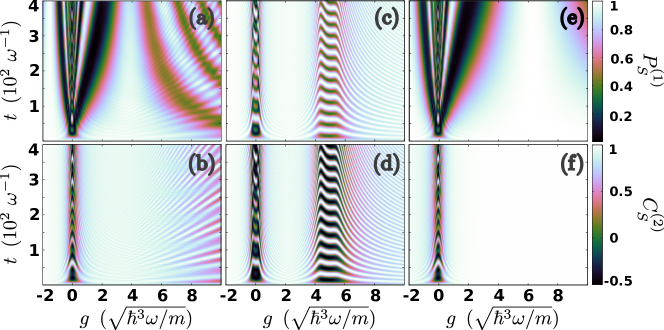
Figure 1: Time evolution of (a), (c), (e) the spin polarization magnitude $P_{S}^{(1)}$ and (b), (d), (f) the spin-spin correlator $C^{(2)}_{S}$ for varying $g$. The presented results refer to $N=3$ fermions by employing (a), (b) MCTDHF, (c), (d) TDHF and (e), (f) the generalized spin-chain approach.

III.1 Many-Body Correlated Spin-Flip Dynamics

Figures 1(a) and 1(b) present our MB results for the paradigmatic case of $N=3$ fermions obtained via MCTDHF, that enables us to capture all interparticle correlation effects Alon ; Axel ; MLX ; Jenny1 ; Jenny2 ; Fpolarons . The MCTDHF method is a variational, numerically exact, ab initio method for solving the time-dependent MB Schrödinger equation which includes all correlation effects. It is based on expanding the MB wavefunction in terms of a time-dependent variationally optimized basis. In this way it enables us to efficiently truncate the MB Hilbert space relevant for our system by using a computationally feasible basis size. The MCTDHF method exhibits increased numerical efficiency when compared to an expansion relying on a time-independent basis since the number of basis states can be significantly reduced. A detailed discussion on the capabilities and the MB wavefunction ansatz of the above-mentioned method is presented in Appendix A.

For weak repulsive or attractive interactions, $|g|<0.5$, a rapid demagnetization (see the decaying behaviour of $P_{S}^{(1)}$) is observed, accompanied by a loss of the spin alignment, $C^{(2)}_{S}$, at a time scale $\sim 20$. Partial revivals of both $P_{S}^{(1)}$ and $C^{(2)}_{S}$ appear over regular time intervals for later times. Our results for this interaction interval are compliant with the spin-dynamics analyzed in AMR1 ; AMR2 and we shall refer to this regime as the weak-$g$ demagnetization regime. Indeed within this regime each of the particles precesses with a different Larmor frequency leading to the loss of the polarization magnitude $P^{(1)}_{S}$ after a few precession cycles. For intermediate interactions of either sign, i.e. $0.5<|g|<4$, the decay and revival of $P_{S}^{(1)}$ also occurs but at a drastically increased time-scale (which increases further for larger $|g|$) when compared to the weak-$g$ demagnetization regime. In contrast, $C^{(2)}_{S}$ indicates that the spins are close to be maximally aligned (e.g. $C^{(2)}_{S}\geq 0.85$ for $2<g<4$ and $C^{(2)}_{S}\geq 0.95$ for $g\sim-2$ in Fig. 1(b)) throughout the evolution, signifying ferromagnetic spin-correlations. Therefore, ferromagnetism is unstable in this interaction interval as the polarization ($P^{(1)}_{S}$) of the ensemble features large fluctuations despite the ferromagnetic order captured by $C^{(2)}_{S}$ which is almost perfect. Hence, we refer to this regime as ferromagnetically ordered. In particular, it involves a different spin-order than ferromagnetism, as its order is inferred by the ferromagnetic spin-spin correlations rather than the polarization. For $g>4$ a suppression of the ferromagnetic spin-spin correlations occurs as the amplitude of the $C^{(2)}_{S}$ oscillations increases for stronger $g$, see Fig. 1(b). For instance, at $g\approx 10$, $C^{(2)}_{S}$ fluctuates between the values $0.5$ and unity. $P^{(1)}_{S}$ is also oscillatory taking values between unity and $1/3$, with a significantly smaller oscillation frequency than $C^{(2)}_{S}$ [see Fig. 1(a)]. In the following this interaction interval ($g>4$) is referred to as the strong-$g$ demagnetization regime.

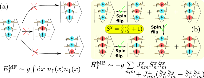
Figure 2: Spin-flip transitions of a spin-polarized few-fermion gas. (a) According to HF each $N$-body state corresponds to a single $N$-body (determinantal) configuration sketched here by the kets. For increasing interaction strength $g$, states with anti-oriented spins accumulate large interaction energies $E_{I}^{\rm HF}$ that forbid spin-flip transitions from the fully polarized state (see crossed arrows). (b) In the MB case the interaction part of the Hamiltonian $H_{I}^{\rm MB}$ for small spin-flip coupling and $g$ approaches a XXZ model AMR1 , which allows for spin-flip transitions between all states with maximal total spin $S^{2}$.

III.2 Spin-Flip Dynamics Within TDHF

To demonstrate the crucial role of correlations within the MB dynamics we compare the above MB findings with the TDHF approximation presented in Fig. 1(c) and 1(d). For weak $|g|$ ($|g|<0.5$) the demagnetization dynamics is qualitatively captured by the TDHF approximation. However, upon increasing $|g|$, (in particular for $0.5<|g|<4$) TDHF predicts no loss of $P^{(1)}_{S}$ in contrast to the MB case [compare Fig. 1(a) and 1(c)], while a similar spin-correlation dynamics is observed [compare Fig. 1(b) and 1(d)]. This behaviour of the TDHF can be interpreted in terms of the Stoner model Stoner ; Salasnich , see Fig. 2(a). Indeed, within HF the interaction energy of contact interacting spin-$1/2$ fermions is proportional to the density overlap between the two spin-components Stoner ; Salasnich . Therefore, for large enough $g$ the system initialized in a spin-polarized state characterized by zero interaction energy, cannot access states with a single (or more) spin-flips due to their large interaction energy. Thus, each of the spins has to preccess with the same frequency resulting in the constant polarization magnitude, $P^{(1)}_{S}$. For strong $g>4$, Rabi oscillations between the ferromagnetic initial state $|\Psi_{F}\rangle$ (characterized by $P^{(1)}_{S}=1$, $C^{(2)}_{S}=1$) and the paired HF ground states $|\Psi^{\rm HF}_{\alpha}\rangle\sim\int{\rm d}^{3}x~{}\phi_{0}(x_{1})\phi_{0}(x_{2})\phi_{1}(x_{3})\psi^{\dagger}_{\uparrow}(x_{1})\psi^{\dagger}_{\downarrow}(x_{2})\psi^{\dagger}_{\alpha}(x_{3})|0\rangle$ (referring to $P^{(1)}_{S}=1/3$, $C^{(2)}_{S}=-1/2$) take place. This indicates that the interparticle repulsion between the paired fermions exactly balances the energy benefit of their pairing in the same state and corresponds to the Stoner instability of the ground state. It is important to note here that these Rabi oscillations are absent in the MB case, see also Fig. 1(c) and 1(d) for $g\approx 5$.

Concluding, the ferromagnetically ordered regime exhibited in the MB case corresponds to a stable ferromagnetic one within the HF framework. This observation exposes the correlated nature of the ferromagnetically ordered regime. In both cases the interaction regime is limited to intermediate values of $g$ and in particular to $0.5<|g|<4$ [see Fig. 1(b), 1(d)]. However, for $g>4$ the mechanism that breaks the spin-order differs. In the HF case the ground state Stoner instability takes place which is forbidden for any finite repulsive interaction in the MB case Lieb ; Sowinski . Instead, it is known that the unpaired states of maximum $S$ [see Fig. 1(b)] and the MB antiferromagnetic ground states exhibit a crossing in the Tonks-Girardeau limit ZurnAntiferro ; Blume ; BrouzosFer ; Buignion ; Lewenstein ; Zinner . In our case due to the breaking of the SU(2) symmetry the above consist an avoided crossing Cui_ref1 ; Ref1_1 ; Ref1_2 which is approached for increasing $g>4$. As we shall argue in section IIID, the fluctuations of $C^{(2)}_{S}$ in the strong-$g$ demagnetization regime for the MB case can be attributed to this avoided crossing.

III.3 Effective Spin-Chain Model

To uncover the main mechanisms responsible for the emergence of the ferromagnetically ordered regime ($0.5<|g|<4$) we employ an extended version of the spin-chain model (see appendix C) presented in Ref. AMR1 . Our spin-chain model incorporates additional effective magnetic field terms (for details see appendix C) when compared to AMR1 , that are necessary for the treatment of generic spin-$1/2$ fermion systems with a single conserved spin-component (here $\hat{S}_{x}$). Within this model the $N$-body wavefuntion is decomposed as $|\Psi(t)\rangle=\sum_{\vec{n}}|\Psi_{\vec{n}}(t)\rangle$ with $|\Psi_{\vec{n}}(t)\rangle=\sum_{\vec{\alpha}}A_{\vec{n};\vec{\alpha}}(t)\hat{c}_{n_{1}\alpha_{1}}^{\dagger}\dots\hat{c}_{n_{N}\alpha_{N}}^{\dagger}|0\rangle$. The operator $\hat{c}_{n\alpha}^{\dagger}$ creates a fermion in the eigenstate $\ket{\chi_{n}^{\alpha}}=\int dx~{}\chi^{\alpha}_{n}(x)\hat{\psi}^{\dagger}_{\alpha}(x)\ket{0}$ of $\hat{H}_{0}+\hat{H}_{S}$, see Eq. (1) and (6). $\vec{n}=(n_{1},\dots,n_{N})$ and $\vec{\alpha}=(\alpha_{1},\dots,\alpha_{N})$ denote the spatial and spin configuration respectively. The crucial approximation in this model is that all the interaction terms, $\hat{H}^{\delta\vec{n}}_{I}$, that couple different spatial configurations $\vec{n}$ can be neglected. By setting $\hat{H}_{I}^{\rm eff}\equiv\hat{H}_{I}-\hat{H}^{\delta\vec{n}}_{I}$, the different spatial configurations $\vec{n}$ are decoupled. It can be shown that the time-evolution of each $|\Psi_{\vec{n}}(t)\rangle$ can be described by an XXZ spin-chain consisting of $N$-spins AMR1 . The employed approximation limits the expected range of validity of the spin-chain model to small interaction values, $g<\sqrt{\hbar\omega^{3}/m}=1$, where the interaction energy is smaller than the energy spacing between the single-particle eigenstates.

The polarization dynamics within the spin-chain model comply with the MB results within the weak-$g$ demagnetization ($|g|<0.5$) and the ferromagnetically ordered regime ($0.5<|g|<4$) [compare Fig. 1(e) and Fig. 1(a)]. Moreover, by comparing $C^{(2)}_{S}$ [see Fig. 1(b) and 1(f)] between the two methods we observe that the spin-correlation dynamics is almost identical in the weak-$g$ demagnetization regime, where the approximations that the spin-chain model employs are valid. On the contrary, in the ferromagnetically ordered regime the ferromagnetic spin-correlations are overestimated by the spin-chain method [hardly visible in Fig. 1(b) and 1(f)]. Finally, for increasing interactions ($g>4$) no strong-$g$ demagnetization regime appears within the spin-chain model, signifying the break down of its validity. This behaviour is clearly imprinted in $C^{(2)}_{S}$ for large $g$ [compare Fig. 1(f) and 1(b) for $g\approx 8$]. To interpret the spin-chain dynamics in the ferromagnetic and strong-$g$ demagnetization regime we note that the configuration $\vec{n}=(0,1,2)$ possesses approximately $99.72\%$ of the contribution to $|\Psi(0)\rangle$ and thus it almost completely dictates the dynamics of the system within the spin-chain approximation. The MB polarization $P^{(1)}_{S}$ dynamics within the ferromagnetically ordered regime is well-captured by the spin-chain model allowing us to conclude that this behaviour emerges due to the spin-dynamics of the different states (characterized by distinct $\vec{\alpha}$) within the dominant $\vec{n}=(0,1,2)$ spatial configuration. In contrast, the (small) depletion of $C_{S}^{(2)}$ in the same regime [see Fig. 1(b)] is absent in the spin-chain approximation, leading to the conclusion that it stems from the neglected couplings to different spatial configurations, contained in $\hat{H}_{I}^{\delta\vec{n}}$. The latter couplings, however, are not as strong as to prohibit the spin-chain model to capture the spin-order emerging within the MB evolution in this interaction regime. Regarding the absence of a strong-$g$ demagnetization regime we remark here that the coupling between the antiferromagnetic ground states belonging to the spatial configuration $\vec{n}=(0,0,1)$ and the initially populated states of the dominant $\vec{n}=(0,1,2)$ configuration is neglected by the spin-chain model.

At this point it becomes clear that the ferromagnetic order exhibited in 1D spin-1/2 Fermi gases greatly deviates from the standard HF description. Additionally, the emerging spin-order is different than the one perceived as ferromagnetic in the literature. Indeed, its defining characteristic is the stability of the spin-spin correlations rather than the polarization. The spin-chain model seems to capture well some of the characteristics of this emerging order. In the following by analyzing in parallel the MB and spin-chain dynamics we will shed light onto the underlying microscopic mechanisms of the ferromagnetically ordered regime.

III.4 Analysis Of The Microscopic Mechanisms

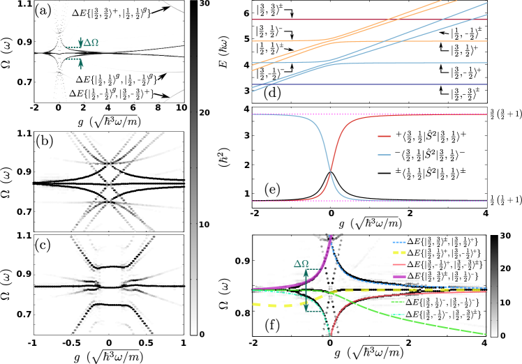
Figure 3: (a), (b) Spectrum of the polarization vector $\mathcal{F}\{P_{S}^{(1)}\}$ for $N=3$ fermions within MCTDHF. $|\frac{1}{2},\pm\frac{1}{2}\rangle^{g}$ refers to the antiferromagnetic ground states. (c) $\mathcal{F}\{P_{S}^{(1)}\}$ within TDHF. (d) Eigenspectrum for all states within the $\vec{n}=(0,1,2)$ configuration within the spin-chain model. (e) Expectation value of the $\hat{S}^{2}$ operator for selected eigenstates of the spin-chain model. The dotted lines indicate the value of $\langle\hat{S}^{2}\rangle$ for $S=\frac{1}{2}$ and $S=\frac{3}{2}$. (f) Comparison of (a) with the eigenenergy differences within the spin-chain model.

To identify the underlying mechanisms of the MB spin-dynamics we invoke the spectrum of the spin-polarization, namely $\mathcal{F}\{P_{S}^{(1)}\}(\Omega)=\big{|}\int{\rm d}t~{}e^{i\Omega t}P^{(1)}_{S}(t)\big{|}^{2}$, presented in Fig. 3(a) and 3(b) for $-2<g<10$ and $|g|<1$ respectively. Recall that each branch in the spectrum of $P_{S}^{(1)}$ corresponds to an energy difference between two eigenenergies of $\hat{H}$, [see Eq. (5)]. For $g=0$ three distinct Larmor frequencies occur that correspond to the three energy differences among the occupied single-particle eigenstates in the spatial configuration $\vec{n}=(0,1,2)$. For $g\neq 0$ a multitude of interaction-dependent frequency branches emerge from each Larmor frequency. The failure of TDHF to capture even on the qualitative level the spin dynamics even for low $g$ is evident in $\mathcal{F}\{P_{S}^{(1)}\}(\Omega)$. Indeed, the TDHF captures only one frequency per particle for $|g|<0.1$ [see Fig. 3(c)] in contrast to the multitude of interaction-dependent frequency branches emerging from each Larmor frequency in the correlated case [see Fig. 3(b)]. Thus we can conclude that the build up of correlations in the MB case even for very small $g$ completely invalidates the HF picture for the spin dynamics. Such correlations are of particular importance in the ferromagnetically ordered regime. In this case, three dominant branches appear in the vicinity of $\Omega\approx 0.85$ [see also Fig. 3(b) for $g\approx 1$] within the correlated case that lead to the beating dynamics of $P^{(1)}_{S}$, observed in Fig. 1(a), 1(b).

The origin of the above-mentioned frequencies can be exposed by comparing $\mathcal{F}\{P_{S}^{(1)}\}$, with the energy differences of the eigenstates of the spin-chain model. As anticipated by our discussion in section IIIC the eigenstates of the configuration $\vec{n}=(0,1,2)$ are expected to well capture the $P^{(1)}_{S}$ dynamics. The eigenspectrum of the spin-chain Hamiltonian $\hat{H}_{\vec{n}}=\hat{H}_{(0,1,2)}$ is presented in Fig. 3(d). The spin-chain eigenstates within the weak-$g$ demagnetization regime ($|g|<0.5$) are ordered in terms of increasing $S_{x}$ due to the Zeeman effect induced by the effective magnetic field along the $x$ axis that $\hat{H}_{S}$, Eq. (6), introduces. Within this weak-$g$ demagnetization regime an avoided crossing between the distinct eigenstates of the same $S_{x}=\pm\frac{1}{2}$ occurs which can be attributed to the breaking of the $\hat{S}^{2}$ symmetry by the inhomogeneity of the $\hat{H}_{S}$ term. The states of the spin-chain model can be labeled as $|S,S_{x}\rangle^{\ell}$ in the repulsive ($\ell=+$) and attractive ($\ell=-$) part of the ferromagnetically ordered regime ($0.5<|g|<4$). This is possible because $S$ is an approximate good quantum number within this interaction range. This property can be identified by examining the expectation value of $\langle\hat{S}^{2}\rangle\equiv{}^{\ell}\langle S,S_{x}|\hat{S}^{2}|S,S_{x}\rangle^{\ell}$. Figure 3(e) presents this expectation value for the states with $S_{x}=\frac{1}{2}$ and varying interaction strength. It becomes evident that for increasing $|g|$ the $\langle\hat{S}^{2}\rangle$ of one of these states [i.e. $|\frac{3}{2},\frac{1}{2}\rangle^{+}$ and $|\frac{3}{2},\frac{1}{2}\rangle^{-}$ in the case of $g>0$ and $g<0$ respectively] approaches the value $\langle\hat{S}^{2}\rangle=\frac{3}{2}\langle\frac{3}{2}+1\rangle$, indicating that $S\approx\frac{3}{2}$. Moreover, the states $\{|\frac{3}{2},\frac{1}{2}\rangle^{-},|\frac{3}{2},\frac{1}{2}\rangle^{\pm}\}$ and $\{|\frac{3}{2},\frac{1}{2}\rangle^{+},|\frac{3}{2},\frac{1}{2}\rangle^{\pm}\}$ in the case of $g>0$ and $g<0$ respectively tend to $\langle\hat{S}^{2}\rangle=\frac{1}{2}(\frac{1}{2}+1)$. We remark here that the states with $S_{x}=-\frac{1}{2}$ exhibit a similar behavior as the aforementioned $S_{x}=\frac{1}{2}$ case and the eigenstates $|\frac{3}{2},\pm\frac{3}{2}\rangle^{\pm}$ correspond to fully polarized states along the $x$ axis with $\langle\hat{S}^{2}\rangle=\frac{3}{2}\langle\frac{3}{2}+1\rangle$ for all $g$ (not shown here for brevity). By employing the spin-chain eigenspectrum, Fig. 3(d), we can identify all the energy branches appearing in Fig. 3(b) with the corresponding eigenenergy differences of the spin-chain model. Most importantly, Fig. 3(f) presents this identification within the ferromagnetically ordered regime ($0.5<|g|<4$). As it can be seen the energy differences between the spin-chain eigenstates with $S\approx\frac{3}{2}$, $\Delta E\{|\frac{3}{2},S_{x}\rangle^{\ell},|\frac{3}{2},S^{\prime}_{x}\rangle^{\ell^{\prime}}\}$, possess the main contribution to $\mathcal{F}\{P_{S}^{(1)}\}$ in the ferromagnetically ordered regime as they match well with the dominant energy branches appearing in the MB dynamics. Based on this identification we can draw several conclusions regarding the order exhibited within the ferromagnetically ordered regime. First, the ferromagnetic spin-correlations emanate from the predominant occupation of MB eigenstates with $S\approx 3/2$ each characterized by a different value of $S_{x}$. The frequency difference $\Delta\Omega$ between the highest ($\Delta E\{|\frac{3}{2},\frac{3}{2}\rangle^{\pm},|\frac{3}{2},\frac{1}{2}\rangle^{l}$) and lowest lying ($\Delta E\{|\frac{3}{2},-\frac{1}{2}\rangle^{l},|\frac{3}{2},-\frac{3}{2}\rangle^{\pm}$) of the above-mentioned dominant branches [see also Fig. 3(d)] results in the dephasing of the initial superposition. In terms of the spin-$\uparrow$ and spin-$\downarrow$ states this means that the system performs spin-flips between the different states with $S=\frac{3}{2}(\frac{3}{2}+1)$ and varying $S_{z}$ leading to the decay of $P^{(1)}_{S}$, see Fig. 2(b). The corresponding timescale is $\tau_{D}\approx\frac{\pi}{\Delta\Omega}$. $\Delta\Omega$ is attributed to the energy shift of the $|\frac{3}{2},\pm\frac{1}{2}\rangle^{\ell}$ states from being equidistantly spaced which is induced by an avoided crossing at $g=0$, as in Fig. 3(d). The increase of $|g|$ within the ferromagnetically ordered regime, leads to a decrease of $\Delta\Omega$ (or equivalently increase of $\tau_{D}$) giving rise to the observed $P_{S}^{(1)}$ dynamics [Fig. 1(a) and 1(e)].

Regarding the strong-$g$ demagnetization regime [see Fig. 3(a) for $g>4$] the frequency branches that correspond to the $|\frac{3}{2},\pm\frac{1}{2}\rangle^{+}$ states deviate from $\Omega\approx 0.85$ as they couple to the antiferromagnetic ground states of $S\approx\frac{1}{2}$ and $S_{x}=\pm\frac{1}{2}$ character. Due to the same mechanism additional branches also appear in $\mathcal{F}\{P^{(1)}_{S}\}$ [see the corresponding arrows in Fig. 3(a)] that contribute to the complex $P^{(1)}_{S}$ dynamics exhibited in this interaction regime [see Fig. 1(a)] and results in the oscillatory patterns of $C_{S}^{(2)}$ [see Fig. 1(b), and also our discussion in section IIIB].

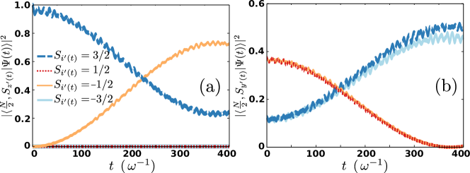
Figure 4: Time evolution of the populations of the $|\frac{3}{2},S_{i^{\prime}(t)}\rangle$ states of the $\vec{n}=(0,1,2)$ configuration for $N=3$, $g=2$ within MCTDHF. (a) $i^{\prime}(t)=z^{\prime}(t)$ and (b) $i^{\prime}(t)=y^{\prime}(t)$.

III.5 Characterization of Entanglement In The Ferromagnetically Ordered Regime

The separation of the energy scales $\Delta\Omega\sim 0.05$ [see Fig. 3(c)] and the average Larmor frequency, $\Omega_{L}=\frac{1}{3\hbar}\Delta E\{|\frac{3}{2},\frac{3}{2}\rangle,|\frac{3}{2},-\frac{3}{2}\rangle\}\sim 0.85$ observed in Fig. 3, enables us to further characterize the superpositions that emerge in the ferromagnetically ordered regime. To this end we introduce the precessing bases $|\frac{3}{2},S_{j^{\prime}(t)}\rangle=e^{i\frac{1}{2}\hat{S}_{x}\Omega_{L}t}|\frac{3}{2},S_{j}\rangle$ ($j\in\{x,y,z\}$) and project the MB wavefunction obtained within MCTDHF to these basis states. Note that if all the particles were collectively precessing with the frequency $\Omega_{L}$ then $|\langle\frac{3}{2},S_{z^{\prime}(t)}=\frac{3}{2}|\Psi(t)\rangle|$ would be constant in time. However, as we have already enstablished in section IIIB, this is not the case. Fig. 4(a) presents the results of this projection for a representative case ($g=2$) within the ferromagnetically ordered regime. We observe a low-frequency ($\sim\Delta\Omega$) population transfer from the state $|\frac{3}{2},S_{z^{\prime}(t)}=\frac{3}{2}\rangle$ to the state $|\frac{3}{2},S_{z^{\prime}(t)}=-\frac{1}{2}\rangle$. For $t>350$ the latter mechanism results in $\langle\hat{S}_{z^{\prime}(t)}\rangle\approx 0$, as $|\frac{3}{2},S_{z^{\prime}(t)}=-\frac{1}{2}\rangle$ possesses approximatively a three times larger population as compared to $|\frac{3}{2},S_{z^{\prime}(t)}=\frac{3}{2}\rangle$. The nature of this superposition can be understood by transforming to the orthogonal precessing axis, $y^{\prime}(t)$ [see Fig. 4(b)]. In this case the populations of $|\frac{3}{2},S_{y^{\prime}(t)}=\frac{3}{2}\rangle$ and $|\frac{3}{2},S_{y^{\prime}(t)}=-\frac{3}{2}\rangle$ are almost equal for $t>350$, signifying the tendency to dynamically approach a NOON state, characterized by $\langle\hat{S}_{y^{\prime}(t)}\rangle\approx 0$, i.e. $|\Psi(t_{0})\rangle\sim\frac{1}{\sqrt{2}}(|\frac{3}{2},S_{y^{\prime}(t)}=\frac{3}{2}\rangle+e^{i\phi}|\frac{3}{2},S_{y^{\prime}(t)}=-\frac{3}{2}\rangle)$ with a relative phase $\phi$. These results combined with the conserved quantity $\langle\hat{S}_{x}\rangle=0$ explain the decay of the total magnetization $P^{(1)}_{S}\to 0$ for $t>350$. Accordingly, the spin-dynamics within the ferromagnetically ordered regime describes the dynamical evolution of a fully-polarized state to a superposition one consisting of two antiparallel-oriented fully-polarized states.

IV SPIN DYNAMICS FOR $\mathbf{N=5}$ FERMIONS

We next demonstrate the robustness of our main findings for the case of larger particle numbers by examining a system consisting of $N=5$ fermions.

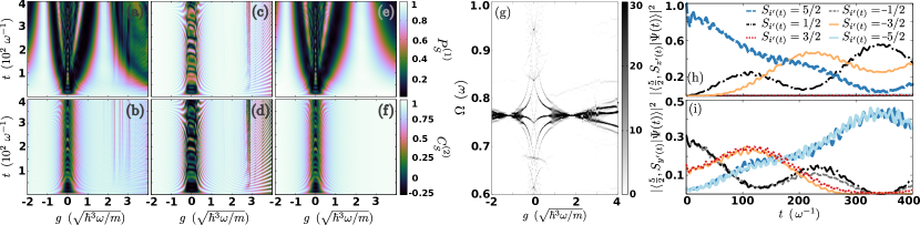
Figure 5: Time evolution of (a), (c), (e) the spin polarization magnitude $P_{S}^{(1)}$ and (b), (d), (f) the spin-spin correlator $C^{(2)}_{S}$ for varying $g$. The presented results refer to $N=5$ fermions by employing (a), (b) the MCTDHF, (c), (d) the TDHF and (e), (f) the generalized spin-chain approach. (g) Spectrum of the polarization vector $\mathcal{F}\{P_{S}^{(1)}\}$ for $N=5$ fermions within MCTDHF. Time evolution of the populations of the $|\frac{5}{2},S_{i^{\prime}(t)}\rangle$ states of the $\vec{n}=(0,1,2,3,4)$ configuration for $N=5$, $g=1$ within MCTDHF. (h) $i^{\prime}(t)=z^{\prime}(t)$ and (i) $i^{\prime}(t)=y^{\prime}(t)$.

Figures 5(a)-5(f) present $P^{(1)}_{S}$ and $C^{(2)}_{S}$ for $N=5$ fermions within the tree different approaches employed above, i.e. the MCTDHF, TDHF and spin-chain approach. A similar spin-dynamics as for the $N=3$ case is observed for both quantities, but in different interaction regimes, caused by the increase of $N$. The ferromagnetically ordered regime occurs in the range $0.5<|g|<2$, where both $P^{(1)}_{S}$ and $C^{(2)}_{S}$ possess a value proximal to unity within the TDHF approach [see Fig. 5(c) and 5(d)]. In the same range the MB treatment provided by MCTDHF reveals that $P^{(1)}_{S}$ is decaying [see Fig. 5(a)], a feature which is also well captured by the spin-chain method [see Fig. 5(e)]. The only additional structures that emerge in the MB spin-flip dynamics when compared to the $N=3$ case are very narrow interaction windows where $C^{(2)}_{S}$ gets significantly depleted from unity [see Fig. 5(b), $g\approx 2.5$]. These regions can be attributed to avoided crossings between the different spin-states of the dominant spatial configuration $\vec{n}=(0,1,2,3,4)$ with states characterized by spatial configurations with double occupations of single-particle spatial mode(s) [e.g. $\vec{n}^{\prime}=(0,1,2,2,3)$].

Inspecting $\mathcal{F}\{P^{(1)}_{S}\}$ for $N=5$ fermions, see Fig. 5(g), similar microscopic mechanisms to the $N=3$ case can be observed in both the weak-$g$ and the ferromagnetically ordered regime. Despite the fact that more states are involved, the main features essentially remain the same. The weak-$g$ demagnetization regime originates from the multitude of branches emerging from the five available non-interacting Larmor frequencies. However, only five (which can be identified as the energy differences between the $|\frac{5}{2},S^{x}\rangle^{\ell}$ states) possess a significant amplitude for $|g|>0.5$. The frequency difference, $\Delta\Omega$, between the highest and lowest lying of the above five branches [see Fig. 5(g)] gives rise to the decay of $P_{S}^{(1)}$ within the ferromagnetically ordered regime observed in Fig. 5(a).

Finally, we show that even the superpositions emerging in the dynamics are of the same character as for $N=3$ fermions. To reveal this we construct the precessing basis analogously to the case $N=3$, namely $|\frac{5}{2},S_{j}^{\prime}(t)\rangle=e^{i\frac{1}{2}\hat{S}_{x}\Omega_{L}t}|\frac{5}{2},S_{j}\rangle$, $\Omega_{L}=\frac{1}{5\hbar}\Delta E\{|\frac{5}{2},\frac{5}{2}\rangle,|\frac{5}{2},-\frac{5}{2}\rangle\}$ and expand the MB wavefunction in terms of the latter. Figures 5(h) and 5(i) present the results of this expansion for the axes $z^{\prime}(t)$ and $y^{\prime}(t)$ respectively and for $g=1$ within the ferromagnetically ordered regime. Figure 5(h) demonstrates that the collective precession of the spins characterized by $|\langle\frac{5}{2},S_{z^{\prime}(t)}=\frac{5}{2}|\Psi(t)\rangle|^{2}=1$ gets quickly dephased. At later times $t\approx 350$ the dephasing of the collective Larmor precession leads to the formation of a NOON-like state characterized by $|\langle\frac{5}{2},S_{y^{\prime}(t)}=\frac{5}{2}|\Psi(t)\rangle|^{2}=|\langle\frac{5}{2},S_{y^{\prime}(t)}=-\frac{5}{2}|\Psi(t)\rangle|^{2}\approx 1/2$ [see Fig. 5(i)], compliant with our $N=3$ results.

V GENERALIZATION TO OTHER DYNAMICAL SYSTEMS

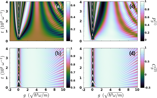
Figure 6: Time evolution of (a), (c) the spin polarization magnitude $P^{(1)}_{S}$ and (b), (d) the spin-spin correlator $C^{(2)}_{S}$ for varying $g$. The presented $N=3$ results are derived within MCTDHF (a), (b) with $|\Psi(0)\rangle=|\Psi_{S=3/2,Sz=1/2}\rangle$ as initial state (see text) and by employing the Hamiltonian $\hat{H}$ or (c), (d) with $|\Psi(0)\rangle=|\Psi_{0}\rangle$ and $\hat{\tilde{H}}+\hat{H}^{\prime}_{S}$.

Below we demonstrate that the above identified ferromagnetic properties are not restricted to the previously examined out-of-equilibrium scenario. Indeed, we will show that the 1D spin-$1/2$ Fermi gas exhibits a similar spin-dynamics for different initial states characterized by $S\approx\frac{N}{2}$ within the ferromagnetic-like regime, which, furthermore, does not depend on the exact form of the Rabi coupling potential. The special feature of the specific dynamical protocol investigated in the previous sections is that it can be readily implemented in state-of-the-art experiments (see also section VI).

It can be shown that any initial state which is dominated by the states of the $\vec{n}=(0,\dots,N-1)$ spatial configuration with $S=\frac{N}{2}$ possesses a similar spin-spin correlation dynamics to the ferromagnetic one, $|\Psi_{F}\rangle=\prod_{i=0}^{2}\int{\rm d}x~{}\phi_{i}(x)\hat{\psi}^{\dagger}_{\uparrow}(x)|0\rangle$. The reason is that the time-evolution of the expectation value of $\hat{S}^{2}$ reads

$$\langle\Psi(t)|\hat{S}^{2}|\Psi(t)\rangle=\sum_{S_{x}=-\frac{N}{2}}^{\frac{N}{2}}\bigg{|}\Big{\langle}\Psi(t)\Big{|}\frac{3}{2};S_{x}\Big{\rangle}\bigg{|}^{2}\bigg{\langle}\frac{3}{2};S_{x}\bigg{|}e^{\frac{it}{\hbar}\hat{H}}\hat{S}^{2}e^{-\frac{it}{\hbar}\hat{H}}\bigg{|}\frac{3}{2};S_{x}\bigg{\rangle}+\mathcal{O}\left(1-\sum_{S_{x}=-\frac{N}{2}}^{\frac{N}{2}}\bigg{|}\Big{\langle}\Psi(t)\Big{|}\frac{3}{2};S_{x}\Big{\rangle}\bigg{|}^{2}\right).$$ (7)

This equation stems from the fact that the quantum numbers $S=\frac{N}{2}$ and $S_{x}\in\{-\frac{N}{2},\dots,\frac{N}{2}\}$ uniquely identify a single $N$-body state of the $\vec{n}=(0,\dots,N-1)$ configuration. Additionally, the $\hat{S}_{x}$ operator commutes with both $\hat{S}^{2}$ and $\hat{H}$ canceling all cross terms that would appear in the first term of Eq. (7). Therefore, within the ferromagnetically ordered regime where $\langle\Psi(t)|\hat{S}^{2}|\Psi(t)\rangle\approx\frac{N}{2}\left(\frac{N}{2}+1\right)$, for $|\Psi(0)\rangle=|\Psi_{F}\rangle$, all of the contributing expectation values need to satisfy $\langle\frac{N}{2};S_{x}|e^{\frac{it}{\hbar}\hat{H}}\hat{S}^{2}e^{-\frac{it}{\hbar}\hat{H}}|\frac{N}{2};S_{x}\rangle\approx\frac{N}{2}\left(\frac{N}{2}+1\right)$, since the probabilities are positive definite, i.e. $|\langle\Psi(t)|\frac{3}{2};S_{x}\rangle|^{2}>0$. This implies that for all initial states which satisfy $\sum_{S_{x}=-\frac{N}{2}}^{\frac{N}{2}}|\langle\Psi(0)|\frac{3}{2};S_{x}\rangle|^{2}\approx 1$ the correlation dynamics within the ferromagnetically ordered regime is stable.

To provide concrete numerical evidence supporting the above-mentioned theoretical argument, we present in Fig. 6, the time-evolution of the polarization, $P^{(1)}_{S}$, and the spin-spin correlator, $C^{(2)}_{S}$, utilizing the Hamiltonian of Eq. (5), in the case of the initial state ZurnAntiferro

$$|\Psi_{S=3/2,Sz=1/2}\rangle=\int\frac{{\rm d}^{3}x}{\sqrt{3!}}\begin{vmatrix}\phi_{0}(x_{1})&&\phi_{0}(x_{2})&&\phi_{0}(x_{3})\\ \phi_{1}(x_{1})&&\phi_{1}(x_{2})&&\phi_{1}(x_{3})\\ \phi_{2}(x_{1})&&\phi_{2}(x_{2})&&\phi_{2}(x_{3})\end{vmatrix}\hat{\psi}^{\dagger}_{\uparrow}(x_{1})\hat{\psi}^{\dagger}_{\uparrow}(x_{2})\hat{\psi}_{\downarrow}^{\dagger}(x_{3})|0\rangle.$$ (8)

As it can be clearly seen the correlation dynamics [see Fig 6(b)] is almost identical to the one observed in section IIIA for the fully spin-polarized initial state, $|\Psi_{F}\rangle=\prod_{i=0}^{2}\int{\rm d}x~{}\phi_{i}(x)\hat{\psi}^{\dagger}_{\uparrow}(x)|0\rangle$ [see also Fig. 1(b)]. Most importantly, the ferromagnetically ordered regime appears in the $0.5<|g|<4$ interaction range, characterized by $C^{2}_{S}\approx 1$, while losses of spin-alignment (i.e. $C^{2}_{S}<1$) are found outside of this interaction regime. The polarization dynamics [see Fig 6(a)], however, shows different patterns from the dynamics obtained with $|\Psi_{F}\rangle$, since the initial polarization in the present case is $P^{(2)}_{S}=\frac{1}{3}$ rather than unity. Nevertheless, within the ferromagnetically ordered regime we observe large fluctuations of the polarization while the spin-spin correlator is almost constant, similarly to the dynamics that the system with $|\Psi(0)\langle=|\Psi_{F}\rangle$ follows [see Fig. 1 (a), (b)].

According to our previous discussion (see Section II) the Rabi-coupling between the spin-$\uparrow$ and the spin-$\downarrow$ states is assumed to be weak and the characteristic length of its modulation is larger than the length scale of the trap, $\sqrt{\frac{\hbar}{m\omega}}$. Due to these assumptions it is reasonable to approximate the Rabi-coupling potential by its Taylor series. We can, thus, demonstrate that our results generalize to all Rabi-coupling potentials with a non-vanishing second-order derivative by showing that a similar dynamics as in section IIIA can be obtained for the parabolic spin-coupling potential

$$\hat{H}^{\prime}_{S}=\frac{1}{2}m(\Delta\omega)^{2}\int{\rm d}x~{}x^{2}\sum_{\alpha,\beta}\hat{\psi}_{\alpha}^{\dagger}(x)\sigma^{x}_{\alpha\beta}\hat{\psi}_{\beta}(x).$$ (9)

For our simulations we employ $\Delta\omega=\sqrt{0.1}$, while the system is initialized in the fully polarized state, $|\Psi_{F}\rangle$, though as argued above a similar dynamics takes place when the system is initialized in the $|\Psi_{S=3/2,Sz=1/2}\rangle$ state (results not shown here for brevity). As it can be seen, the behaviour of the system in terms of the spin-polarization, $P^{(1)}_{S}$ [see Fig. 6(c)] and the spin-spin correlations, $C^{(2)}_{S}$ [see Fig. 6(d)] is almost identical to the case of $\hat{H}_{S}$, Eq. (6) [see also Fig. 1(a) and 1(b)], with deviations occurring only within the $g\approx 0$ region [compare Fig. 6(c) and 1(b)]. We also note that in the case of strong spin-dependent potentials, where the exact shape of the Rabi-coupling potential might play an important role, spin segregation phenomena are induced AMR1 ; AMR2 . These compete with the ferromagnetic order identified here, as the overlap of the spin-densities provides an upper bound for $\langle\hat{S}^{2}\rangle$ and therefore such investigations lie beyond the scope of this work.

VI EXPERIMENTAL REALIZATION

Our setup can be realized using ⁴⁰K atoms under the influence of a Raman coupling of the two energetically lowest hyperfine states, while the observables $P^{(1)}_{S}$ and $C^{(2)}_{S}$ are accessible by fluorescence imaging. Below we propose a possible experimental realization in order to probe our findings. The robustness of the suggested measurement scheme is demonstrated by comparing our MCTDHF results with simulated sets of single-shot images that contain additional noise emulating this way the noise sources inherent in a corresponding experiment Heidelberg ; BrouzosJochim ; ZurnAntiferro .

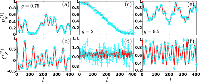
Figure 7: (a), (c), (e) Comparison of $P^{(1)}_{S}$ as calculated by MCTDHF (solid lines) and the average of $600$ single-shot measurements (data points with error bars) within each of the dynamical regimes. For the single-shot simulations the error $\Delta\phi=\pi/12$ has been incorporated. (b), (d), (f) Similar to (a), (c), (e) but for $C^{(2)}_{S}$. All quantities are given in harmonic units, error bars correspond to an uncertainty of one standard deviation.

The effective Rabi coupling scheme, see $\hat{H}_{S}$ Eq. (6), can be achieved by employing a two-photon resonant, $\delta=0$, Raman transition via two Gaussian focussed laser beams. To incorporate non-negligible interatomic interactions one needs to apply a bias magnetic field close to the point of an $s$-wave broad Fano-Feshbach resonance Chin . For ⁴⁰K atoms a broad $s$-wave Fano-Feshbach resonance between the hyperfine states $|\uparrow\rangle=|{}^{2}S_{1/2};F=\frac{9}{2},m_{F}=-\frac{9}{2}\rangle$ and $|\downarrow\rangle=|{}^{2}S_{1/2};F=\frac{9}{2},m_{F}=-\frac{7}{2}\rangle$, is located at the magnetic field strength $B_{\rm FF}=202.10$ G Greinersup .

Fluorescence imaging is commonly used to probe the state of the system in few-atom ($N<10$) experiments Heidelberg . Here a certain number of atoms is ejected from the trap and recaptured into a magneto-optical trap Pethicksup . Subsequently, the number of ejected particles can be inferred by measuring the intensity of the scattered light. We show that $P^{(1)}_{S}$ and $C^{(2)}_{S}$ can be experimentally detected using fluorescence imaging. $P^{(1)}_{S}$ and $C^{(2)}_{S}$ depend on the average and the variance of the magnitude of the spin polarization respectively. Because of the employed Raman scheme the Hamiltonian (6) is implemented in the interaction picture. This implies that in the Schrödinger picture and in the absence of the Raman fields the orientation of the spin-vector precesses around the $z$ spin-axis with frequency $\omega_{\uparrow\downarrow}=2\pi\times\left[44.8+0.156{\rm G}^{-1}~{}(B-B_{\rm FF})\right]$MHz (where $B$ refers to the bias magnetic field). $\omega_{\uparrow\downarrow}$ corresponds to the energy offset between the $|\uparrow\rangle$ and $|\downarrow\rangle$ states of ⁴⁰K for magnetic fields in the vicinity of $B_{\rm FF}$. As a consequence only the spin-polarization along the $z$ axis (i.e. population-imbalance in the occupation of the hyperfine states $|\uparrow\rangle$, $|\downarrow\rangle$) in spin-space can be directly probed. To measure the spin-state in such atomic systems Ramsay spectroscopy is employed to coherently rotate the rotating $x$ or $y$ axes in the interaction picture to the stationary $z$ axis, which is common for both pictures. A Ramsay spectroscopy sequence (described in the interaction picture) is utilized. Initially all of the atoms are prepared in the $N$-body state $|\Psi(0)\rangle$, namely all atoms reside in the $|\uparrow\rangle$ hyperfine state. At time $t=0$ the inhomogeneous Raman coupling of the hyperfine states is suddenly switched on and the fermions are exposed to it for time $t$. By the end of this process, the MB wavefunction has evolved from $|\Psi(0)\rangle$ to $|\Psi(t)\rangle$ (in the interaction picture) under the influence of $\hat{H}$. At time $t$, the Raman coupling is suddenly switched off and the system evolves for a dark time $t_{\rm dark}$. Within this time interval the reestablished symmetries of the Hamiltonian $\hat{H}_{0}+\hat{H}_{I}$ [see Eq. (3), (4)] prohibit any change to $\bm{S}$ and $S^{2}$. To measure the $S_{x}$ or $S_{y}$ components we need to rotate the desired spin component to the $z$ axis by applying a $-\sigma_{y}$ or $\sigma_{x}$, $\frac{\pi}{2}$-pulse respectively by means of spatially homogeneous two-photon-resonant optical Raman fields with the appropriate phase shift, $\phi$, from the inhomogeneous one (for $S_{z}$ no $\frac{\pi}{2}$-pulse is used and the sequence continues directly with the next step). This sequence stops the precession dynamics of the desired spin component in the Schrödinger picture as it is mapped to the stationary $z$ axis. In the following, all the spin-$\downarrow$ are removed from the trap by applying a high-intensity resonant laser pulse at time $t_{\rm ex}$ ZurnAntiferro . The surviving atoms are loaded into the magneto-optical trap (at $t=t_{\rm meas}$) and counted to provide a measurement for the spin polarization $S_{i}=\frac{2N_{\uparrow}-N}{2}$ along the selected axis $i\in\{x,y,z\}$ .

As a proof-of-principle of the above mentioned imaging procedure we simulate single experimental measurements, where we take into account a random error in the phase $\Delta\phi$. We employ a generalized version of the recent single-shot implementation offered by Multi-Layer Multi-Configuration Hartree method for atomic Mixtures (ML-MCTDHX) MLX (see kasparsup ; Lodesup ; filled_vortexsup ; Lianew and appendix B for details) and evaluate $P_{S}^{(1)}$ and $C^{(2)}_{S}$ from the simulated experimental data. Note that $\Delta\phi$ might be induced by variations in the optical path of the $-\sigma_{y}$ or $\sigma_{x}$, $\frac{\pi}{2}$-pulse Raman beams. To incorporate this source of error we simulate experimental measurements for each of the $x$, $y$ and $z$ components of the spin vector and incorporate a random rotation by $\delta\phi$ along the $z$ axis that follows a Gaussian distribution of width $\Delta\phi$.

Figures 7(a) and 7(b) offer a comparison of our MCTDHF data with the simulated experimental estimates based on $600$ single-shot realizations containing an error $\Delta\phi=\pi/12$. We observe that despite the latter error the single-shot results follow closely the MCTDHF data and reproduce both the spin polarization $P_{S}^{(1)}$, as well as, the correlation dynamics $C^{(2)}_{S}$. The uncertainty of the simulated single-shot results is of the order $\sim 0.05$. Agreement between the MCTDHF data and the single-shot estimates is observed also for the ferromagnetically ordered [see Fig. 7(c) and 7(d)] and the strong-$g$ demagnetization regime [see Fig. 7(e) and 7(f)]. Therefore, we conclude that the error in the phase $\phi$ is not prohibitive for accurate measurements of $P^{(1)}_{S}$ and $C^{(2)}_{S}$ as long as it is kept sufficiently smaller than $\frac{\pi}{2}$.

VII SUMMARY AND OUTLOOK

We have explored the spin-flip dynamics of few ultracold fermions subject to spatially inhomogeneous external driving of the spins. In particular, we showed that in this case the polarization of the confined Fermi gas cannot be stabilized for any interaction strength. A result that lies in contrast to the picture of ferromagnetism provided by the celebrated Stoner model. Most importantly, a stable correlation-induced ferromagnetic spin-order emerges in spite of the strongly fluctuating polarization for moderate interactions. We have characterized the emerging spin-order by comparing ab initio simulations with an effective spin-chain model in the few-body case. The influence of correlations and the emergence of entangled NOON-like states during the dynamical evolution of the system has been explicitly demonstrated. In the weak and strong interaction limit the behavior of the system is characterized by a significant depletion of the spin-spin correlator which can be related to the corresponding avoided crossings appearing in the eigenspectrum. Our setup is experimentally accessible in ⁴⁰K few-atom experiments by employing a Raman coupling scheme of the two energetically lowest hyperfine states. The observables $P_{S}^{(1)}$ and $C_{S}^{(1)}$ can be measured by employing Ramsay spectroscopy and fluorescence imaging.

It is known that the properties of itinerant magnetism vary depending on the confining potential Zintchenko . Studying the stability of ferromagnetism in the case of a double well potential or an optical lattice can yield further insights into the magnetic properties exhibited in one dimensional systems. Notice, also, that the spin-chain model presented here is easily extendable to higher dimensional settings. The investigation on whether a similar order occurs in higher dimensional settings also provides an intriguing perspective for future study. Another interesting prospect is to examine the demagnetization dynamics of few-fermions when exposed to Rashba and Dresselhaus spin-orbit coupling Rashba ; Dresselhaus . This might establish a link to relevant condensed matter systems where such demagnetization mechanisms are well-studied Dyakonov1 ; Elliot ; Yafet . Such dynamics have recently been examined in the case of thermal Fermi gases in the collisionless regime Radic ; Natu ; Stanescu .

Appendix A The Computational Method: ML-MCTDHX and the Spinor Variant of MCTDHF

Our approach to solve the MB Schrödinger equation $\left({i\hbar{\partial_{t}}-\hat{H}}\right)|\Psi(t)\rangle=0$ relies on the Multi-layer Multi-Configuration Time-Dependent Hartree method for atomic Mixtures MLX (ML-MCTDHX). In particular we employ a reduction of the ML-MCTDHX method for spin-$1/2$ fermions being referred in the following as the spinor-variant of Multi-Configuration Time-Dependent Hartree method for Fermions (MCTDHF). MCTDHF has been applied extensively for the treatment of fermions with or without spin-degrees of freedom, in a large class of condensed matter, atomic and molecular physics scenarios (see e.g. Zanghellinisup ; Katosup ; Caillatsup ; Nestsup ; Bonitzsup ; Haxtonsup ) and recently also applied in the field of ultracold atoms Axel ; MLX ; Jenny1 ; Jenny2 ; Fpolarons ; CaoMistakidis . The key idea of MCTDHF lies in the usage of a time-dependent (t-d) and variationally optimized MB basis set, which allows for the optimal truncation of the total Hilbert space. The ansatz for the MB wavefunction is taken as a linear combination of t-d Slater determinants $|\vec{n}(t)\rangle$, with t-d weight coefficients $A_{\vec{n}}(t)$

$$|\Psi(t)\rangle=\sum_{\vec{n}}A_{\vec{n}}(t)|\vec{n}(t)\rangle.$$ (10)

Each t-d Slater determinant is expanded in terms of $M$ t-d variationally optimized single-particle functions (SPFs) $\left|\phi_{l}(t)\right\rangle$, $l=1,2,\dots,M$ with occupation numbers $\vec{n}=(n_{1},\dots,n_{M})$. The SPFs are subsequently expanded in a primitive basis $\{\left|k,s\right\rangle\}$, being the tensor product of a discrete variable representation (DVR) basis for the spatial degrees of freedom $\{|k\rangle\}$ of dimension $M_{p}$ and the two-dimensional spin basis $\{|\uparrow\rangle,|\downarrow\rangle\}$

$$|\phi_{j}(t)\rangle=\sum_{k=1}^{M_{p}}\sum_{\alpha=\{\uparrow,\downarrow\}}C^{j}_{k\alpha}(t)\ket{k}\ket{\alpha}.$$ (11)

$C^{j}_{k\alpha}(t)$ refer to the corresponding t-d expansion coefficients. Note here that each t-d SPF is a general spinor wavefunction of the form $|\phi_{j}(t)\rangle=\int{\rm d}x~{}[\chi_{j}^{\uparrow}(x)\hat{\psi}^{\dagger}_{\uparrow}(x)+\chi_{j}^{\downarrow}(x)\hat{\psi}^{\dagger}_{\downarrow}(x)]|0\rangle$ and hence the employed method is termed as the spinor-variant of MCTDHF. The time-evolution of the $N$-body wavefunction under the effect of the Hamiltonian $\hat{H}$ reduces to the determination of the $A$-vector coefficients and the SPFs, which in turn follow the variationally obtained MCTDHF equations of motion Alon ; Axel ; MLX . In the limiting case of $M=N$, the method reduces to the t-d Hartree-Fock method, while for the case of $M=2M_{p}$, it is equivalent to a full configuration interaction approach (commonly referred to as “exact diagonalization” in the literature) within the basis $\{|k,s\rangle\}$.

For our implementation we have used a harmonic oscillator DVR, which results after a unitary transformation of the commonly employed basis of harmonic oscillator eigenfunctions, as a primitive basis for the spatial part of the SPFs. To study the dynamics, we propagate the wavefunction by utilizing the appropriate Hamiltonian within the MCTDHF equations of motion. To verify the accuracy of the numerical integration, we impose the following overlap criteria $\left|\langle\Psi|\Psi\rangle-1\right|<10^{-8}$ for the total wavefunction and $\left|\langle\varphi_{i}|\varphi_{j}\rangle-\delta_{ij}\right|<10^{-9}$ for the SPFs. To infer about convergence, we increase the number of SPFs and DVR basis states such that the observables of interest ($P_{S}^{(1)}$, $C_{s}^{(2)}$) do not change within a given relative accuracy which is in our case $10^{-4}$. More specifically, we have used $M_{p}=60$, $M=26$ and $M_{p}=80$, $M=20$ for the $N=3$ and the $N=5$ case respectively. Note that a full configuration interaction treatment of the above-mentioned systems in the employed primitive bases would require $280840$ number-states for $N=3$ and $820384032$ ones for $N=5$.

Appendix B Single-Shot Procedure in Spin-$1/2$ Fermi Gases

The single-shot simulation procedure relies on a sampling of the MB probability distribution, being available within the ML-MCTDHX framework. In a spinor Fermi gas the single-shot procedure is altered significantly when compared to the single component case kasparsup ; Lodesup ; filled_vortexsup . Here the role of entanglement between particles in different spin states plays an important role. For example consider the procedure that the spin-$\uparrow$ atoms are imaged before the spin-$\downarrow$ atoms. Then, the total number of spin-$\uparrow$ atoms $N_{\uparrow}^{\rm imag}$ that will be imaged is not a priori known due to the breaking of the $S_{z}$ symmetry. However, after imaging all of the spin-$\uparrow$ atoms the number of spin-$\downarrow$ atoms is exactly known $N_{\downarrow}^{\rm imag}=N-N_{\uparrow}^{\rm imag}$ since the total number of atoms $N$ is definite.

To capture the entanglement between the different spin states the MB wavefunction obtained by ML-MCTDHX should be expressed such that the entanglement between the spin states is evident. The spin-$1/2$ Fermi gas under consideration is a bipartite system Horodecki1sup ; Horodecki2sup since the spatial degree of freedom for each particle in the spin-$\uparrow$ or spin-$\downarrow$ state resides in the Fock space $\mathcal{F}^{\uparrow}$, $\mathcal{F}^{\downarrow}$ respectively. The latter results in a total Fock space $\mathcal{F}^{S=1/2}=\mathcal{F}^{\uparrow}\otimes\mathcal{F}^{\downarrow}$. Then, the MB wavefunction can be expressed in the Schmidt decomposition form (herewith we omit the temporal dependence for simplicity)

$$|\Psi\rangle=\sum_{k=1}^{K}\sqrt{\lambda_{k}}|\Psi_{k}^{\uparrow}\rangle|\Psi_{k}^{\downarrow}\rangle.$$ (12)

The coefficient $\lambda_{k}$ is referred to as the natural occupation of the species function $k$ Note that, $|\Psi_{k}^{\alpha}\rangle\in\mathcal{F}^{\alpha}$ and as such the number of $\alpha$-spin particles varies for different Schmidt modes, $k$. A state of the bipartite system [see Eq. (12)] cannot be expressed as a direct product of two states from the two subsystem Fock spaces $\mathcal{F}^{\alpha}$ if at least two coefficients $\lambda_{k}$ are nonzero. In the latter case the system is referred to as entangled Roncagliasup . The Schmidt decomposition of the MB wavefunction is obtained as follows. The reduced density matrix for one of the spin states, let it be $\alpha$, is evaluated i.e. $\rho^{\alpha}=\mathrm{Tr}_{\alpha^{\prime}}[|\Psi\rangle\langle\Psi|]$, where $\alpha^{\prime}$ refers to the spin state orthogonal to $\alpha$ and subsequently diagonalized resulting in its Schmidt representation $\rho^{\alpha}=\sum_{k=1}^{M}\lambda_{k}|\Psi^{\alpha}_{k}\rangle\langle\Psi^{\alpha}_{k}|$. Then, the corresponding species wavefunction of the spin state $\alpha^{\prime}$ can be calculated by $|\Psi_{k}^{\alpha^{\prime}}\rangle=\frac{1}{\sqrt{\lambda_{k}}}\langle\Psi_{k}^{\alpha}|\Psi\rangle$.

The single-shot process in spinor gases represents a generalization of the single-shot process for a mixture with a definite number of atoms in each species Lianew . This generalization is based on the treatment of the vacuum state $|0^{\alpha}\rangle$. Before each step of the single-shot process the existence of particles in the imaged spin state is checked. To perform the latter a random number in the interval $P_{\rm rand}\in[0,1]$ is compared with $\lambda_{\tilde{k}}$, where $\tilde{k}$ is the Schmidt mode for which $|\Psi^{\alpha}_{\tilde{k}}\rangle=|0^{\alpha}\rangle$ holds. If $P_{\rm rand}<\lambda_{\tilde{k}}$ the imaging of the spin state $\alpha$ ends and the MB wavefunction is projected to $|\tilde{\Psi}\rangle=|0^{\alpha}\rangle\otimes|\Psi^{\alpha^{\prime}}_{\tilde{k}}\rangle$. Then the simulation of the imaging of the $\alpha^{\prime}$ spin state is initiated. The MB wavefunction in this case is the species wavefunction $|\Psi^{\alpha^{\prime}}_{\tilde{k}}\rangle$ and as such the single-shot procedure reduces to the well-established single species case (see kasparsup ; Lodesup ; filled_vortexsup and also the discussion below). For $P_{\rm rand}>\lambda_{\tilde{k}}$ a particle in the spin state $\alpha$ is imaged. First, a random position is drawn according to the constraint $\rho_{\alpha}^{(1)}(x_{1}^{\prime})=\langle\Psi|\hat{\psi}^{\dagger}_{\alpha}(x_{1}^{\prime})\hat{\psi}_{\alpha}(x_{1}^{\prime})|\Psi\rangle>l_{1}$ where $l_{1}$ refers to a random number within the interval [$0$, max{$\rho^{(1)}_{\alpha}(x)\}$]. Then we project the $N$-body wavefunction to the ($N-1$)-body one by employing the operator $\frac{1}{\mathcal{N}}\hat{\psi}_{\alpha}(x_{1}^{\prime})$, where $\mathcal{N}=\sqrt{\langle\Psi|\hat{\psi}^{\dagger}_{\alpha}(x_{1}^{\prime})\hat{\psi}_{\alpha}(x_{1}^{\prime})|\Psi\rangle}$ is a normalization factor. The latter process directly affects the Schmidt coefficients $\lambda_{k}$’s (entanglement weights) and thus despite the fact that the spin-$\alpha^{\prime}$ atoms have not been imaged yet, both $\rho_{\uparrow}^{(1)}(x)=\langle\Psi|\hat{\psi}^{\dagger}_{\uparrow}(x)\hat{\psi}_{\uparrow}(x)|\Psi\rangle$ and $\rho_{\downarrow}^{(1)}(x)=\langle\Psi|\hat{\psi}^{\dagger}_{\downarrow}(x)\hat{\psi}_{\downarrow}(x)|\Psi\rangle$ change. This can be easily understood by employing again the Schmidt decomposition. Indeed after this first measurement the ($N-1$)-particle MB wavefunction reads

$$\ket{\tilde{\Psi}^{(-1)}}=\sum_{k}\sqrt{\tilde{\lambda}_{k}^{(-1)}}\ket{\tilde{\Psi}_{k}^{\alpha(-1)}}\ket{\Psi_{k}^{\alpha^{\prime}}},$$ (13)

where $\ket{\tilde{\Psi}_{k}^{\alpha(-1)}}=\frac{1}{N_{i}}\hat{\psi}_{\alpha}(x_{1}^{\prime})\ket{\Psi_{k}^{\alpha}}$ refer to the species wavefunction after the imaging and $N_{k}=\sqrt{\bra{\Psi_{k}^{\alpha}}\hat{\psi}_{\alpha}^{\dagger}(x_{1}^{\prime})\hat{\psi}_{\alpha}(x_{1}^{\prime})\ket{\Psi_{k}^{\alpha}}}$ denotes the corresponding normalization factor. Finally, the Schmidt coefficients read $\tilde{\lambda}^{(-1)}_{k}=\lambda_{k}N_{k}/\sum_{m}\lambda_{m}N_{m}^{2}$. The above-mentioned procedure is repeated $N^{\rm imag}_{\alpha}$ times until the condition $||\langle 0^{\alpha}|\Psi^{(-N^{\rm imag}_{\alpha})}\rangle||=1$ is reached or if a random number satisfying $P_{\rm rand}<\lambda_{\tilde{k}}^{(-N^{\rm imag}_{\alpha})}$ is selected. The resulting distribution of positions ($x^{\prime}_{1}$, …,$x^{\prime}_{N^{\rm imag}_{\alpha}}$) is convoluted with a point spread function leading to a single-shot $\mathcal{A}^{\alpha}(\tilde{x})$ for the spatial configuration of spin-$\alpha$ particles, where $\tilde{x}$ refers to the spatial coordinates within the image. It is worth mentioning at this point that, in the special case for which the probability of $N^{\rm imag}_{\alpha}=N$ is zero, it can be easily shown that upon annihilating the last spin-$\alpha$ particle (provided that $P_{\rm rand}>\lambda^{(-N_{\alpha}^{\rm imag}+1)}_{\tilde{k}}$ is chosen) the $(N-N_{\alpha}^{\rm imag})$-particle MB wavefunction becomes

$$\ket{\tilde{\Psi}^{(-N^{\rm imag}_{\alpha})}}=\ket{0^{\alpha}}\otimes\hskip 10.0pt\sum_{k\neq\tilde{k}}\frac{\sqrt{\tilde{\lambda}^{(-N^{\rm imag}_{\alpha}+1)}_{k}}\braket{x^{\prime}_{N_{\alpha}^{\rm imag}}}{\Phi_{k}^{\alpha}}}{\sum\limits_{m\neq\tilde{k}}\sqrt{\tilde{\lambda}^{(-N^{\rm imag}_{\alpha}+1)}_{k}|\braket{x^{\prime}_{N_{\alpha}^{\rm imag}}}{\Phi_{k}^{\alpha}}|^{2}}}\ket{\Psi_{k}^{\alpha^{\prime}}}.$$ (14)

After this last step the entanglement between the spin states has been destroyed and the single component wavefunction of the spin $\alpha^{\prime}$ atoms $\ket{\Psi^{(-N_{\alpha}^{\rm imag})}}$ corresponds to the second term on the right hand side of Eq. (14).

In this way, it becomes evident that after the imaging of spin $\alpha$ particles the resulting wavefunction $\ket{\Psi^{(-N_{\alpha}^{\rm imag})}}=\ket{\Psi^{\alpha^{\prime}}}$ [see Eq. (14)] is a non-entangled ($N-N_{\alpha}^{\rm imag}$)-particle MB wavefunction and its corresponding single-shot procedure is the same as in the single species case kasparsup . The latter is well-established (for details see kasparsup ; Lodesup ) and here it is only briefly outlined below. We first calculate $\rho^{(1)}_{\alpha^{\prime}}(x)$ from the MB wavefunction $\ket{\Psi^{(-N_{\alpha}^{\rm imag})}}=\ket{\Psi^{\alpha^{\prime}}}$. Then, a random position $x^{\prime\prime}_{1}$ is drawn obeying $\rho^{(1)}_{\alpha^{\prime}}(x^{\prime\prime}_{1})>l_{2}$ where $l_{2}$ is a random number in the interval [$0$, $\max[\rho^{(1)}_{\alpha^{\prime}}(x)]$]. Next, one particle located at position $x^{\prime\prime}_{1}$ is annihilated and $\rho^{(1)\prime}_{\alpha^{\prime}}(x)$ is calculated from $\ket{\Psi^{(-N_{\alpha}^{\rm imag}-1)}}=\left[\rho^{(1)}_{\alpha^{\prime}}(x^{\prime\prime}_{1})\right]^{-1/2}\hat{\psi}_{\alpha^{\prime}}(x^{\prime\prime}_{1})\ket{\Psi^{(-N_{\alpha}^{\rm imag})}}$. To proceed, a new random position $x^{\prime\prime}_{2}$ is drawn from $\rho^{(1)\prime}_{\alpha^{\prime}}(x;t_{im})$. Following this procedure for $N-N_{\alpha}^{\rm imag}$ steps we obtain the distribution of positions ($x^{\prime\prime}_{1}$, …,$x^{\prime\prime}_{N-N_{\alpha}^{\rm imag}}$) which is then convoluted with a point spread function resulting in a single-shot image $\mathcal{A}^{\alpha^{\prime}}(\tilde{x}^{\prime}|\mathcal{A}^{\alpha}(\tilde{x}))$.

Appendix C Spin-Chain Approach

The spin-chain Hamiltonian builds upon the spin dependent eigenstates, $|\chi_{n}^{\alpha}\rangle$, of the non-interacting Hamiltonian $\hat{H}_{0}+\hat{H}_{S}$, where $\alpha$, $n$ denote the spin and spatial modes. To simplify the notation below, we perform a rotation in spin-space by employing the unitary operator $\hat{U}=e^{i\frac{\pi}{4}\hat{S}_{y}}$ such that the $x$ axis (see main text) is mapped to the $z$ axis and thus the spin-modes correspond to $\alpha\in\{\uparrow,\downarrow\}$. The $n$-th spatial mode is considered as singly occupied if either $|\chi_{n}^{\uparrow}\rangle$ or $|\chi_{n}^{\downarrow}\rangle$ is occupied, doubly occupied if both are occupied and unoccupied if neither is occupied. Then the spatial configurations are defined by $\vec{n}=(n_{1},\dots,n_{N})$ where $n_{i}$ refers to the occupied spatial modes. There are $2^{N-2D}$ ($D$ denotes the number of double occupations) distinct states that correspond to the same spatial configuration, $\vec{n}$, corresponding to the different available spin-configurations $\vec{\alpha}=(\alpha_{1},\dots,\alpha_{N})$. Consequently, a basis state of the $N$-body system, $|\vec{n};\vec{\alpha}\rangle=\hat{c}^{\dagger}_{n_{1}\alpha_{1}}\dots\hat{c}^{\dagger}_{n_{N}\alpha_{N}}|0\rangle$, is completely defined by its spin and spatial configurations $\vec{\alpha}$ and $\vec{n}$ respectively.

To derive the effective Hamiltonian of the spin-chain model, $\hat{H}^{\rm eff}$, we neglect all terms that couple states of different spatial configurations. The non-interacting Hamiltonian $\hat{H}_{0}+\hat{H}_{S}$ is diagonal on the basis states $|\vec{n},\vec{\alpha}\rangle$ and thus its exact form is incorporated in the effective spin-chain Hamiltonian, $\hat{H}^{\rm eff}$. However, the same is not true for the interaction term $\hat{H}_{I}$. According to the above mentioned approximation, the general form of the effective interaction term, $\hat{H}_{I}^{\rm eff}$, contains all the terms in $\hat{H}_{I}$ that preserve the spatial configuration of the state they act on. There are only two terms in $\hat{H}_{I}$ that possess the latter property and are linearly independent, namely the $\hat{H}_{I}^{\rm shift}$ and $\hat{H}_{I}^{\rm exc}$ terms. $\hat{H}_{I}^{\rm shift}=g\sum_{m,n=0}^{m_{\rm max}}u_{mm}^{nn}\hat{c}^{\dagger}_{n\uparrow}\hat{c}^{\dagger}_{m\downarrow}\hat{c}_{m\downarrow}\hat{c}_{n\uparrow}$ accounts for the energy shift of the single-particle modes due to interaction, where $u^{nq}_{mp}=\int dx~{}[\chi^{\uparrow}_{n}(x)\chi^{\downarrow}_{m}(x)]^{*}\chi^{\downarrow}_{p}(x)\chi^{\uparrow}_{q}(x)$ denote the corresponding interaction integrals. $\hat{H}_{I}^{\rm exc}=g\sum_{m=0}^{m_{\rm max}}\sum_{n\neq m}u^{mn}_{nm}\hat{c}^{\dagger}_{m\uparrow}\hat{c}^{\dagger}_{n\downarrow}\hat{c}_{m\downarrow}\hat{c}_{n\uparrow}$ allows for the exchange of the single-particle modes after a collision event. Therefore, the effective Hamiltonian reads $\hat{H}^{\rm eff}=\hat{H}_{0}+\hat{H}_{S}+\hat{H}_{I}^{\rm eff}$, where $\hat{H}_{I}^{\rm eff}=\hat{H}_{I}^{\rm shift}+\hat{H}_{I}^{\rm exc}$.

To cast $\hat{H}^{\rm eff}$ in the spin-chain form we define the spin operators for each spatial mode $\hat{\sigma}^{0}_{n}=\hat{c}_{n\uparrow}^{\dagger}\hat{c}_{n\uparrow}+\hat{c}_{n\downarrow}^{\dagger}\hat{c}_{n\downarrow}$, $\hat{\sigma}^{z}_{n}=\hat{c}_{n\uparrow}^{\dagger}\hat{c}_{n\uparrow}-\hat{c}_{n\downarrow}^{\dagger}\hat{c}_{n\downarrow}$, $\hat{\sigma}^{+}_{n}=\hat{c}_{n\uparrow}^{\dagger}\hat{c}_{n\downarrow}$ and $\hat{\sigma}^{-}_{n}=\hat{c}_{n\downarrow}^{\dagger}\hat{c}_{n\uparrow}$. The effective MB Hamiltonian $\hat{H}^{\rm eff}$ conserves the spatial modes for each spatial configuration $\vec{n}=(n_{1},\dots,n_{N})$ as it commutes with the projection operators

$$\hat{P}_{\vec{n}}=\sum_{\alpha_{1}=\{\uparrow,\downarrow\}}\dots\sum_{\alpha_{N}=\{\uparrow,\downarrow\}}\hskip 2.0pt\hat{c}^{\dagger}_{n_{1}\alpha_{1}}\dots\hat{c}^{\dagger}_{n_{N}\alpha_{N}}\hskip 2.0pt|0\rangle\langle 0|\hat{c}_{n_{N}\alpha_{N}}\dots\hat{c}_{n_{1}\alpha_{1}}.$$ (15)

Employing this projection operator, we can derive the spin-chain Hamiltonian, $\hat{H}_{\vec{n}}=\hat{P}_{\vec{n}}\hat{H}^{\rm eff}\hat{P}_{\vec{n}}$, for each configuration $\vec{n}$ with no double occupations (i.e. $n_{i}\neq n_{j}$, $\forall~{}i,j$), corresponding to the $N$-spin XXZ spin-chain

$$\hat{H}_{\vec{n}}=\varepsilon_{\vec{n}}(g)+\sum_{i=1}^{N}h_{n_{i}}(g)\hat{\sigma}^{z}_{n_{i}}-g\sum_{i=1}^{N-1}\sum_{j=i+1}^{N}\bigg{[}\left(J^{\perp}_{n_{i}n_{j}}\hat{\sigma}^{+}_{n_{i}}\hat{\sigma}^{-}_{n_{j}}+J^{\perp*}_{n_{i}n_{j}}\hat{\sigma}^{-}_{n_{i}}\hat{\sigma}^{+}_{n_{j}}\right)+J^{z}_{n_{i}n_{j}}\hat{\sigma}^{z}_{n_{i}}\hat{\sigma}^{z}_{n_{j}}\bigg{]}.$$ (16)

The spin-spin interactions are given by the overlap integrals $J_{nm}^{\perp}=u^{mn}_{nm}$ and $J_{nm}^{z}=\frac{1}{4}(u^{nn}_{mm}+u_{nn}^{mm})$. The interaction-dependent energy shift $\varepsilon_{\vec{n}}(g)$ and the local magnetic field $h_{n_{i}}(g)$ read

$$\begin{split}\varepsilon_{\vec{n}}(g)&=\sum_{i=1}^{N}\frac{E_{n_{i}}^{\uparrow}+E_{n_{i}}^{\downarrow}}{2}+g\sum_{i=1}^{N-1}\sum_{j=i+1}^{N}J^{z}_{n_{i}n_{j}},\\ h_{n_{i}}(g)&=\frac{E_{n_{i}}^{\uparrow}-E_{n_{i}}^{\downarrow}}{2}+g\sum_{j=1,~{}j\neq i}^{N}\frac{u^{n_{i}n_{i}}_{n_{j}n_{j}}-u_{n_{i}n_{i}}^{n_{j}n_{j}}}{4}.\end{split}$$ (17)

The configurations with $D$ double occupations have to be treated separately because the creation operator of a double occupancy $\hat{c}^{\dagger}_{n\uparrow}\hat{c}^{\dagger}_{n\downarrow}$ possesses a non-trivial commutation relation with the $\hat{\sigma}^{0}_{n}$ one, $[\hat{\sigma}^{0}_{m},\hat{c}^{\dagger}_{n\uparrow}\hat{c}^{\dagger}_{n\downarrow}]=2\delta_{nm}\hat{c}^{\dagger}_{n\uparrow}\hat{c}^{\dagger}_{n\downarrow}$. In this case, it turns out that the projected Hamiltonian, $\hat{H}_{\vec{n}}$, is expressed in terms of a $(N-2D)$-spin XXZ Hamiltonian, $\hat{H}_{\vec{m}}^{(2D)}$, with $\vec{m}$ being a $(N-2D)$-particle configuration composed of the singly occupied states of $\vec{n}$. The $\hat{H}_{\vec{n}}$ and $\hat{H}_{\vec{m}}^{(2D)}$ are related via the creation operator of all the double occupations $\hat{\mathcal{M}}^{\dagger}_{\vec{k}}\equiv\prod_{j=0}^{D-1}\hat{c}^{\dagger}_{k_{j}\downarrow}\hat{c}^{\dagger}_{k_{j}\uparrow}$, where $\vec{k}$ is the vector of doubly occupied modes in $\vec{n}$, as $\hat{H}_{\vec{n}}=\hat{\mathcal{M}}^{\dagger}_{\vec{k}}\hat{H}_{\vec{m}}^{(2D)}\hat{\mathcal{M}}_{\vec{k}}$. $\hat{H}_{\vec{m}}^{(2D)}$ has exactly the same form as Eq. (16) but the energy shift, $\varepsilon_{\vec{m}}^{(2D)}(g)$, and local magnetic field, $h^{(2D)}_{m_{i}}(g)$, possess additional contributions when compared to the ones in Eq. (17). Namely,

$$\begin{split}\varepsilon_{\vec{m}}^{(2D)}(g)=&\varepsilon_{\vec{m}}(g)+\sum_{i=1}^{D}2\varepsilon^{0}_{k_{i}}+g\Bigg{[}\sum_{i=1}^{D}2J^{z}_{k_{i}k_{i}}+\sum_{i=1}^{D-1}\sum_{j=i+1}^{D}4J^{z}_{k_{i}k_{j}}+\sum_{i=1}^{D}\sum_{j=1}^{N-2D}J^{z}_{k_{i}m_{j}}\Bigg{]},\\ h^{(2D)}_{m_{i}}(g)=&h_{m_{i}}(g)+g\sum_{j=1}^{D}\frac{u^{m_{i}m_{i}}_{k_{j}k_{j}}-u_{m_{i}m_{i}}^{k_{j}k_{j}}}{2}.\end{split}$$ (18)

The weight of each spatial configuration to the MB wavefunction $|\Psi(t)\rangle$ is constant in time as the $w_{\vec{n}}=\langle\Psi(t)|\hat{P}_{\vec{n}}|\Psi(t)\rangle$ are conserved. Therefore, the time evolution of the MB wavefunction within the spin-chain approximation reads

$$|\Psi(t)\rangle=\sum_{\vec{n}}\sqrt{w_{\vec{n}}}~{}e^{-i\hat{H}_{\vec{n}}t}|\Psi_{\vec{n}}(0)\rangle,$$ (19)

where $|\Psi_{\vec{n}}(0)\rangle=\frac{1}{\sqrt{w_{\vec{n}}}}\hat{P}_{\vec{n}}|\Psi(0)\rangle$ is the normalized initial wavefunction for each XXZ spin-chain.

The generalization of the presented method compared to the one developed in Ref. AMR1 is the inclusion of the interaction-dependent local magnetic potential [see Eq. (16) and (18)], which vanish for a linear gradient as the one considered in Ref. AMR1 in the present case such a term is important for obtaining the correct behaviour of the polarization magnitude $P^{(1)}_{S}$ in the ferromagnetically ordered regime. Within our implementation we numerically diagonalize the one-body Hamiltonian, $\hat{H}_{0}+\hat{H}_{S}$, by employing the basis consisting of the $80$ energetically lowest eigenstates of the harmonic oscillator and truncate the summation over $\vec{n}$ of Eq. (19) by taking into account only the contributions of spatial mode configurations with $|w_{\vec{n}}|>10^{-12}$. This truncation results in $1520$ and $38304$ configurations for $N=3$ and $N=5$ fermions respectively.

- (1) D. Vollhardt, N. Blumer, and M. Kollar, Metallic Ferromagnetism - An Electronic Correlation Phenomenon, Lecture Notes in Physics Vol. 580, Springer (2001).
- (2) M. Brando, D. Belitz, F. M. Grosche, and T. R. Kirkpatrick, Rev. Mod. Phys. 88, 025006 (2016).
- (3) S. Sachdev, Nat. Phys. 4, 173 (2008).
- (4) E. Stoner, Philos. Mag. 15, 1018 (1933).
- (5) G.-B. Jo, Y.-R. Lee, J.-H. Choi, C. A. Christensen, T. H. Kim, J. H. Thywissen, D. E. Pritchard, and W. Ketterle, Science 325, 1521 (2009).
- (6) C. Sanner, E. J. Su, W. Huang, A. Keshet, J. Gillen, and W. Ketterle, Phys. Rev. Lett. 108, 240404 (2012).
- (7) D. Pekker, M. Babadi, R. Sensarma, N. Zinner, L. Pollet, M. W. Zwierlein, and E. Demler, Phys. Rev. Lett. 106, 050402 (2011).
- (8) A. Amico, F. Scazza, G. Valtolina, P. E. S. Tavares, W. Ketterle, M. Inguscio, G. Roati, and M. Zaccanti, Phys. Rev. Lett. 121, 253602 (2018).
- (9) C. Chin, R. Grimm, P. Julienne, and E. Tiesinga, Rev. Mod. Phys. 82, 1225 (2010).
- (10) C. Kohstall, M. Zaccanti, M. Jag, A. Trenkwalder, P. Massignan, G. M. Bruun, F. Schreck, and R. Grimm, Nature (London) 485, 615 (2012).
- (11) F. Scazza, G. Valtolina, P. Massignan, A. Recati, A. Amico, A. Burchianti, C. Fort, M. Inguscio, M. Zaccanti, and G. Roati, Phys. Rev. Lett. 118, 083602 (2017).
- (12) W. Li and X. Cui, Phys. Rev. A 96, 053609 (2017).
- (13) G. Valtolina, F. Scazza, A. Amico, A. Burchianti, A. Recati, T. Enss, M. Inguscio, M. Zaccanti, and G. Roati, Nat. Phys. 13, 709 (2017).
- (14) F. Serwane, G. Zürn, T. Lompe, T. B. Ottenstein, A. N. Wenz, and S. Jochim, Science 332, 336 (2011).
- (15) A. N. Wenz, G. Zürn, S. Murmann, I. Brouzos, T. Lompe, and S. Jochim, Science 342, 457 (2013).
- (16) S. Murmann, F. Deuretzbacher, G. Zürn, J. Bjerlin, S. M. Reimann, L. Santos, T. Lompe, and S. Jochim, Phys. Rev. Lett. 115, 215301 (2015).
- (17) S. E. Gharashi and D. Blume, Phys. Rev. Lett. 111, 045302 (2013).
- (18) I. Brouzos and P. Schmelcher, Phys. Rev. A 87, 023605 (2013).
- (19) P. O. Bugnion and G. J. Conduit, Phys. Rev. A 87, 060502(R) (2013).
- (20) T. Sowiński, T. Grass, O. Dutta, and M. Lewenstein, Phys. Rev. A 88, 033607 (2013).
- (21) E. J. Lindgren, J. Rotureau, C. Forssén, A. G. Volosniev and N. T. Zinner, New J. Phys. 16, 063003 (2014).
- (22) J. Levinsen, P. Massignan, G. M. Bruun, and M. M. Parish, Sci. Adv. 1, e1500197 (2015).
- (23) F. Deuretzbacher, D. Becker, J. Bjerlin, S. M. Reimann, and L. Santos, Phys. Rev. A 90, 013611 (2014).
- (24) A. G. Volosniev, D. V. Fedorov, A. S. Jensen, M. Valiente, and N. T. Zinner, Nat. Comm. 5, 5300 (2014).
- (25) L. Yang, L. Guan, and H. Pu, Phys. Rev. A 91, 043634 (2015).
- (26) X. Cui and T.-L. Ho, Phys. Rev. A 89, 023611 (2014).
- (27) X. Cui and T.-L. Ho, Phys. Rev. A 89, 013629 (2014).
- (28) A. P. Koller, M. L. Wall, J. Mundinger, and A. M. Rey, Phys. Rev. Lett. 117, 195302 (2016).
- (29) P. T. Grochowski, T. Karpiuk, M. Brewczyk, and K. Rzążewski, Phys. Rev. Lett. 119, 215303 (2017).
- (30) L. Salasnich and V. Penna, New J. Phys. 19, 043018 (2017).
- (31) V. Penna and L. Salasnich, J. Phys. B: At. Mol. Opt. Phys. 52, 035301 (2019).
- (32) V. Giovannetti, S. Lloyd, and L. Maccone, Nat. Photonics 5, 222-229 (2011).
- (33) J. A. Jones, S. D. Karlen, J. Fitzsimons, A. Ardavan, S. C. Benjamin, G. A. D. Briggs, and J. J. L. Morton, Science 324, 1166 (2009).
- (34) O. E. Alon, A. I. Streltsov, and L. S. Cederbaum, J. Chem. Phys. 127, 154103 (2007).
- (35) E. Fasshauer and A. U. J. Lode, Phys. Rev. A 93, 033635 (2016).
- (36) L. Cao, V. Bolsinger, S. I. Mistakidis, G. M. Koutentakis, S. Krönke, J. M. Schurer, and P. Schmelcher, J. Chem. Phys. 147, 044106 (2017).
- (37) J. Erdmann, S. I. Mistakidis, and P. Schmelcher, Phys. Rev. A 98, 053614 (2018).
- (38) J. Erdmann, S. I. Mistakidis, and P. Schmelcher, Phys. Rev. A 99, 013605 (2019).
- (39) S.I. Mistakidis, G.C. Katsimiga, G.M. Koutentakis, and P. Schmelcher, New J. Phys. 21 043032 (2019).
- (40) M. Olshanii, Phys. Rev. Lett. 81, 938 (1998).
- (41) P. Tommasini, E. J. V. de Passos, A. F. R. de Toledo Piza, M. S. Hussein, and E. Timmermans, Phys. Rev. A 67, 023606 (2003).
- (42) E. Nicklas, H. Strobel, T. Zibold, C. Gross, B. A. Malomed, P. G. Kevrekidis, and M. K. Oberthaler, Phys. Rev. Lett. 107, 193001 (2011).
- (43) D. M. Stamper-Kurn and M. Ueda, Rev. Mod. Phys. 85, 1191 (2013).
- (44) N. R. Bernier, E. G. Dalla Torre, and E. Demler, Phys. Rev. Lett. 113, 065303 (2014).
- (45) A. P. Koller, J. Mundinger, M. L. Wall, and A. M. Rey, Phys. Rev. A 92, 033608 (2015).
- (46) E. Lieb, D. Mattis, Phys. Rev. 125, 164 (1962).
- (47) T. Sowiński, Condens. Matter 3, 7 (2018).
- (48) A. G. Volosniev, D. Petrosyan, M. Valiente, D. V. Fedorov, A. S. Jensen, and N. T. Zinner, Phys. Rev. A 91, 023620 (2015).
- (49) Q. Guan and D. Blume, Phys. Rev. A 92, 023641 (2015).
- (50) C. A. Regal, M. Greiner, and D. S. Jin, Phys. Rev. Lett. 92, 040403 (2004).
- (51) C.J. Pethick and H. Smith, Bose-Einstein condensation in dilute gases, Cambridge University Press (Cambridge, 2002).
- (52) K. Sakmann and M. Kasevich, Nat. Phys. 12, 451 (2016).
- (53) A.U. Lode and C. Bruder, Phys. Rev. Lett. 118, 013603 (2017).
- (54) G. C. Katsimiga, S. I. Mistakidis, G. M. Koutentakis, P. G. Kevrekidis, and P. Schmelcher, New J. Phys. 19 123012 (2017).
- (55) S. I. Mistakidis, G. C. Katsimiga, P. G. Kevrekidis, and P. Schmelcher, New J. Phys. 20, 043052 (2018).
- (56) I. Zintchenko, L. Wang, and M. Troyer, Eur. Phys. J. B, 89, 180 (2016).
- (57) A. Bychkov and E. I. Rashba, J. Phys. C 17, 6039 (1984).
- (58) G. Dresselhaus, Phys. Rev. 100, 580 (1955).
- (59) M. I. Dyakonov and V. I. Perel, Zh. Eksp. Teor. Fiz. 60, 1954 (1971) [Sov. Phys. JETP 33, 1053 (1971)].
- (60) R. J. Elliot, Phys. Rev. 96, 266 (1954).
- (61) Y. Yafet, Phys. Lett. A 98, 287 (1983).
- (62) T. D. Stanescu, C. Zhang, and V. Galitski, Phys. Rev. Lett. 99, 110403 (2007).
- (63) S. S. Natu and S. Das Sarma, Phys. Rev. A 88, 033613 (2013).
- (64) J. Radić, S. S. Natu, and V. Galitski, Phys. Rev. Lett. 112, 095302 (2014).
- (65) J. Zanghellini, M. Kitzler, C. Fabian, T. Brabec, and A. Scrinzi, Laser Phys. 13, 1064 (2003).
- (66) T. Kato and H. Kono, Chem. Phys. Lett. 392, 533 (2004).
- (67) J. Caillat, J. Zanghellini, M. Kitzler, O. Koch, W. Kreuzer, and A. Scrinzi, Phys. Rev. A 71, 012712 (2005).
- (68) M. Nest, T. Klamroth, and P. Saalfrank, J. Chem. Phys. 122, 124102 (2005).
- (69) D. Hochstuhl, S. Bauch, and M. Bonitz, J. Phys.: Conf. Ser. 220, 012019 (2010).
- (70) D. J. Haxton, K. V. Lawler, and C. W. McCurdy, Phys. Rev. A 83, 063416 (2011).
- (71) L. Cao, S. I. Mistakidis, X. Deng, and P. Schmelcher, Chem. Phys. 482, 303 (2017).
- (72) R. Horodecki, P. Horodecki, M. Horodecki, and K. Horodecki, Rev. Mod. Phys. 81, 865 (2009).
- (73) P. Horodecki, R. Horodecki, and M. Horodecki, Act. Phys. Slov. 48, 3 (1998).
- (74) M. Roncaglia, A. Montorsi, and M. Genovese, Phys. Rev. A 90, 062303 (2014).