Equilibrium magnetization of a quasispherical cluster of single-domain particles

Abstract

Equilibrium magnetization curve of a rigid finite-size spherical cluster of single-domain particles is investigated both numerically and analytically. The spatial distribution of particles within the cluster is random. Dipole-dipole interactions between particles are taken into account. The particles are monodisperse. It is shown, using the stochastic Landau-Lifshitz-Gilbert equation, that the magnetization of such clusters is generally lower than predicted by the classical Langevin model. In a broad range of dipolar coupling parameters and particle volume fractions, the cluster magnetization in the weak field limit can be successfully described by the modified mean-field theory, which was originally proposed for the description of concentrated ferrofluids. In moderate and strong fields, the theory overestimates the cluster magnetization. However, predictions of the theory can be improved by adjusting the corresponding mean-field parameter. If magnetic anisotropy of particles is additionally taken into account and if the distribution of the particles’ easy axes is random and uniform, then the cluster equilibrium response is even weaker. The decrease of the magnetization with increasing anisotropy constant is more pronounced at large applied fields. The phenomenological generalization of the modified mean-field theory, that correctly describes this effect for small coupling parameters, is proposed.

I Introduction

Nano- and micro-sized assemblies of single-domain particles are of great interest in modern biotechnology and medicine. Prominent examples are composite magnetic microspheres (or “magnetic beads”) which consist of fine magnetic particles dispersed in or layered onto a spherical (usually polymer or silica) matrix Gijs (2004); Gervald et al. (2010). The diameter of embedded particles can range from several to several dozen nanometers, and the characteristic size of microspheres themselves most commonly ranges from tenths to several microns. One of the most popular applications of magnetic microspheres is the magnetic cell separation – a technique that allows one to magnetically label cells of a specific type and then isolate them from a heterogeneous cell mixture using a gradient field McCloskey et al. (2003); Leong et al. (2016). Also microspheres can be used as magnetically controlled carriers for targeted drug delivery Widder et al. (1978); Dutz et al. (2012) and as force and torque transducers in magnetic tweezers designed to probe mechanical properties of biomolecules Amblard et al. (1996); van Oene et al. (2015).

Another important class of objects are dense three-dimensional (3D) nanoclusters of single-domain particles which are sometimes referred to as “magnetic multicore nanoparticles” Yang et al. (2005); Dutz et al. (2009); Schaller et al. (2009a). Such clusters are typically covered with a non-magnetic protective coating and have a hydrodynamic diameter of 50-200 nm. Multicore nanoparticles can be thought as intermediate between single-domain nanoparticles and magnetic microspheres Dutz (2016). From the viewpoint of cell separation, nanoclusters have some advantages over micrometer-sized beads: for example, they are more stable against sedimentation and have a better binding capacity due to a higher surface-area-to-volume ratio Leong et al. (2016); Xu et al. (2011). Multicore nanoparticles are considered to be perspective for magnetic hyperthermia treatment Dutz et al. (2011); Blanco-Andujar et al. (2015) and magnetic imaging Lartigue et al. (2012); Eberbeck et al. (2013). Aside from their high biomedical potential, magnetic 3D nanoclusters are also interesting due to their presence in some types of ferrofluids Buzmakov and Pshenichnikov (1996); Magnet et al. (2012). It is known that suspended nanoclusters can significantly alter the fluid’s magnetic, mass-transfer and rheological properties Ivanov and Pshenichnikov (2010); Borin et al. (2011).

For simplicity, it is sometimes assumed that microspheres and nanoclusters contain non-interacting and magnetically isotropic single-domain particles Amblard et al. (1996); Ivanov and Pshenichnikov (2010); Borin et al. (2011); Guo et al. (2003). However, in recent years quasi-spherical rigid clusters of different sizes have been actively studied via numerical simulations Schaller et al. (2009a, b); Usov and Serebryakova (2016); Ilg (2017); Weddemann et al. (2010); Melenev et al. (2010); Usov et al. (2017). And it has been repeatedly demonstrated that interactions between embedded particles as well as their magnetic anisotropy can have a noticeable impact on the cluster static Schaller et al. (2009a, b); Usov and Serebryakova (2016); Ilg (2017) and dynamic Ilg (2017); Weddemann et al. (2010); Melenev et al. (2010); Usov et al. (2017) magnetic properties. Particularly, in Refs. Schaller et al. (2009a); Ilg (2017) the equilibrium magnetization curve of a quasi-spherical cluster of uniaxial particles was considered. Dipole-dipole interactions between particles were taken into account. It was demonstrated that for a monodisperse system with a uniform distribution of easy axes the magnetization is generally lower than predicted by the classical Langevin model and that both anisotropy and interactions contribute to the decrease of the cluster equilibrium response.

Though a number of simulation results are currently available, it can be useful to have an analytical model that links properties of particles inside a rigid 3D cluster with the system magnetization. For single-domain particles dispersed in a liquid matrix, many such models exist Huke and Lücke (2004). Among them the so-called “modified mean-field theory” (MMFT) remains one of the most widely used due to its simplicity and accuracy Pshenichnikov et al. (1996); Ivanov and Kuznetsova (2001); Ivanov et al. (2007). In Refs. Wang et al. (2002); Pshenichnikov and Mekhonoshin (2000) it was shown that MMFT also gives correct predictions for the initial susceptibility of magnetoisotropic particles randomly distributed in a solid matrix. Good agreement between simulations and MMFT was obtained for both the bulk system Wang et al. (2002) and the finite spherical cluster Pshenichnikov and Mekhonoshin (2000). The question of whether MMFT is applicable to clusters beyond the weak field limit, to the best of our knowledge, has not been addressed in the literature.

In this paper, the equilibrium magnetization curve of a rigid quasi-spherical cluster of uniaxial particles is studied via Langevin dynamics simulations. In contrast to recent works Schaller et al. (2009a); Ilg (2017), a special attention is paid to the effect of particle volume fraction on the cluster properties. The applicability of MMFT for the description of magnetic 3D clusters is tested. Possible ways to improve the agreement between the analytical model and simulations are discussed.

II Model and methods

II.1 Model formulation

Let us consider an ensemble of $N$ identical spherical single-domain particles randomly distributed within a spherical volume of radius $R$. Positions of particles inside this volume are fixed, particle overlapping is not allowed. Each particle has a diameter $d$ and a magnetic moment $\bm{\mu}$, which can rotate inside the particle, the corresponding unit vector is $\bm{e}=\bm{\mu}/\mu$. The magnitude of the magnetic moment is $\mu=M_{s}v$, where $M_{s}$ is the saturation magnetization of the particle material, $v=(\pi/6)d^{3}$ is the particle volume. Particles have uniaxial magnetic anisotropy, which is characterized by the anisotropy constant $K$ and the easy axis unit vector $\bm{n}$. Each particle has its own fixed vector $\bm{n}$. The orientation distribution of easy axes is random and uniform. Particles interact with each other via dipole-dipole interactions. The described system is further referred to as the “cluster”. The cluster is immobilized inside a non-magnetic medium and subjected to a uniform magnetic field $\bm{H}$ (the corresponding unit vector is $\bm{h}=\bm{H}/H$). The total magnetic energy of the cluster is

$$U=U_{Z}+U_{ani}+U_{dd},$$ (1)

$$U_{Z}=-\mu_{0}\mu H\sum_{i=1}^{N}\bm{e}_{i}\cdot\bm{h},$$ (2)

$$U_{ani}=-Kv\sum_{i=1}^{N}\left(\bm{e}_{i}\cdot\bm{n}_{i}\right)^{2},$$ (3)

$$U_{dd}=-\frac{\mu_{0}\mu^{2}}{4\pi d^{3}}\sum_{\begin{subarray}{c}i=1\end{subarray}}^{N}\sum_{\begin{subarray}{c}j=i+1\end{subarray}}^{N}\left[\frac{3(\bm{e}_{i}\cdot\bm{r}^{*}_{ij})(\bm{e}_{j}\cdot\bm{r}^{*}_{ij})}{r^{*5}_{ij}}-\frac{\bm{e}_{i}\cdot\bm{e}_{j}}{r^{*3}_{ij}}\right],$$ (4)

where $U_{Z}$ is the Zeeman energy, $U_{ani}$ is the magnetic anisotropy energy, $U_{dd}$ is the dipole-dipole interaction energy, the summation in Eqs. (2–4) is over particles in the cluster, $\mu_{0}$ is the magnetic constant, $\bm{r}^{*}_{ij}=\bm{r}_{ij}/d$, $\bm{r}_{ij}$ is the vector between centers of particles $i$ and $j$.

At non-zero temperature $T$, the normalized magnetic moment of the cluster

$$\bm{m}=\frac{1}{N}\sum_{i=1}^{N}\bm{e}_{i}$$ (5)

is a random vector with fluctuating magnitude and direction. The equilibrium magnetization of the cluster can be determined as

$$M=\frac{1}{V}\left\|\left\langle\sum_{i=1}^{N}\bm{\mu}_{i}\right\rangle\right\|=M_{\infty}\Big{\|}\langle\bm{m}\rangle\Big{\|}=M_{\infty}\langle m_{h}\rangle,$$ (6)

where $V=(4\pi/3)R^{3}$ is the cluster volume, $M_{\infty}=\mu N/V$ is the saturation magnetization of the cluster, $m_{h}=\bm{m}\cdot\bm{h}$ is the projection of the cluster moment on the field direction, angle brackets denote a mean value. Equilibrium magnetization of the cluster is determined by several dimensionless parameters. First of all, this is the so-called Langevin parameter

$$\xi=\frac{\mu_{0}\mu H}{k_{B}T},$$ (7)

which is the characteristic ratio between Zeeman and thermal energies, $k_{B}$ is the Boltzmann constant. The dependence of $\langle m_{h}\rangle$ on $\xi$ can be considered as the cluster magnetization curve. Finding this dependency is the main focus of this work. Other key parameters are the anisotropy parameter

$$\sigma=\frac{Kv}{k_{B}T},$$ (8)

the dipolar coupling parameter

$$\lambda=\frac{\mu_{0}\mu^{2}}{4\pi d^{3}k_{B}T},$$ (9)

and the particle volume fraction

$$\varphi=\frac{vN}{V}.$$ (10)

Let us make some estimates based on material parameters for magnetic solids given in Ref. Rosensweig (2002). First of all, it should be noted that dipolar coupling and anisotropy parameters are not independent variables for particles of a given material, $\sigma/\lambda=(24/\mu_{0})K/M^{2}_{s}$ (here we neglect the difference between the particle diameter and the diameter of its magnetic core). For cobalt ferrite ($M_{s}=425~{}\text{kA~{}m}^{-1}$, $K=180$–$200~{}\text{kJ~{}m}^{-3}$), $\sigma/\lambda\simeq 20$; for magnetite ($M_{s}=446~{}\text{kA~{}m}^{-1}$, $K=23$–$41~{}\text{kJ~{}m}^{-3}$), $\sigma/\lambda=2$–$4$. Since iron oxide nanoparticles are more common in biomedical applications Ilg (2017), here we confine ourselves to the cases when $\sigma$ and $\lambda$ are comparable. At $T=300$ K, magnetite nanoparticles with $d=10$ nm have $\lambda\simeq 1.3$, $\xi=1$ corresponds to $H\simeq 14~{}\text{kA~{}m}^{-1}$. The same nanoparticles with $d=13$ nm have $\lambda\simeq 2.9$, $\xi=1$ corresponds to $H\simeq 6.4~{}\text{kA~{}m}^{-1}$. In this work, the following ranges of control parameters are considered: $\xi\leq 10$, $\sigma\leq 10$, $\lambda\leq 3$, $\varphi\leq 0.3$ and $N=10^{2}$–$10^{3}$.

II.2 Limiting case of non-interacting particles

Equilibrium magnetic properties of non-interacting uniaxial particles in a solid matrix were previously discussed in Refs. Bean and Livingston (1959); Raikher (1983); Chantrell et al. (1985); Williams et al. (1993); Mamiya and Nakatani (1998); Cregg and Bessais (1999). Let us briefly recall some results of these works. If interactions between particles can be neglected, i.e. in the limiting cases $\varphi\ll 1$ or $\lambda\ll 1$, the equilibrium magnetization can be derived within the one-particle approximation. The ratio between magnetic and thermal energies for an isolated particle is usually written as

$$\frac{u}{k_{B}T}=-\xi\cos\omega+\sigma\sin^{2}\vartheta,$$ (11)

where $\omega$ is the angle between the particle moment and the field, $\vartheta$ is the angle between the moment and the easy axis. The system magnetization is determined by the average value of $\cos\omega=\bm{e}\cdot\bm{h}$, which can be found as

$$\langle\cos\omega\rangle=\frac{1}{Z}\frac{\partial Z}{\partial\xi},$$ (12)

where $Z$ is the partition function of the particle. If particles have negligible magnetic anisotropy ($\sigma\ll 1$), the partition function is

$$Z=\frac{1}{2}\int_{0}^{\pi}\exp(\xi\cos\omega)\sin\omega d\omega=\frac{\sinh\xi}{\xi},$$ (13)

which, in combination with Eq. (12), gives the well-known Langevin magnetization:

$$\langle m_{h}\rangle=\langle\cos\omega\rangle={\cal L}(\xi),$$ (14)

where ${\cal L}(\xi)\equiv\coth\xi-1/\xi$ is the Langevin function. For uniaxial particles, the partition function and its first derivative can be written in the following single-integral forms Cregg and Bessais (1999):

$$Z= ~{}{\cal J}_{0}(\xi,\sigma,\psi)$$

$$\equiv \int_{0}^{\pi/2}\exp(-\sigma\sin^{2}\vartheta)\cosh(\xi\cos\vartheta\cos\psi)$$

$$\times I_{0}(\xi\sin\vartheta\sin\psi)\sin\vartheta d\vartheta,$$ (15)

$$\frac{\partial Z}{\partial\xi}= ~{}{\cal J}_{1}(\xi,\sigma,\psi)$$

$$\equiv \int_{0}^{\pi/2}\exp(-\sigma\sin^{2}\vartheta)\Big{[}\cosh(\xi\cos\vartheta\cos\psi)$$

$$\times I_{1}(\xi\sin\vartheta\sin\psi)\sin\vartheta\sin\psi+\sinh(\xi\cos\vartheta\cos\psi)$$

$$\times I_{0}(\xi\sin\vartheta\sin\psi)\cos\vartheta\cos\psi\Big{]}\sin\vartheta d\theta,$$ (16)

where $\psi$ is the angle between the field and the easy axis ($\cos\psi=\bm{n}\cdot\bm{h}$), $I_{0}$ and $I_{1}$ are the modified Bessel functions of the first kind of order zero and one, correspondingly. Thus, for an arbitrary particle with a given easy axis orientation $\psi$, the following expression is valid:

$$\langle\cos\omega\rangle=\frac{{\cal J}_{1}(\xi,\sigma,\psi)}{{\cal J}_{0}(\xi,\sigma,\psi)}.$$ (17)

If particles in the system have different orientations of easy axes, then one have to average Eq. (17) over all presented values of $\psi$ to obtain the net magnetization. It was demonstrated in Ref. Raikher (1983) that the distribution of easy axes (the system “orientation texture”) effects the magnetization curve significantly. For the special case of a random uniform distribution, the magnetization is Williams et al. (1993); Cregg and Bessais (1999)

$$\langle m_{h}\rangle={\cal L}_{ani}(\xi,\sigma)\equiv\int_{0}^{\pi/2}\frac{{\cal J}_{1}(\xi,\sigma,\psi)}{{\cal J}_{0}(\xi,\sigma,\psi)}\sin\psi d\psi.$$ (18)

The integral Eq. (18) is denoted here as ${\cal L}_{ani}(\xi,\sigma)$. This function can be considered as a generalization of the standard Langevin function for the case of solid dispersions with random orientation texture. In the limit of negligible anisotropy, two functions coincide, i.e. ${\cal L}_{ani}(\xi,0)={\cal L}(\xi)$. For finite non-zero values of $\xi$ and $\sigma$, ${\cal L}_{ani}(\xi,\sigma)<{\cal L}(\xi)$ Raikher (1983). However, the zero-field slope of the magnetization curve (the initial magnetic susceptibility $\chi$) does not depend on $\sigma$  Bean and Livingston (1959); Chantrell et al. (1985):

$$\chi=\frac{M}{H}\bigg{|}_{H\rightarrow 0}=\frac{\mu_{0}\mu^{2}\varphi}{vk_{B}T}\Bigg{(}\frac{{\cal L}_{ani}(\xi,\sigma)}{\xi}\bigg{|}_{\xi\rightarrow 0}\Bigg{)}\\ =\frac{\mu_{0}\mu^{2}\varphi}{vk_{B}T}\Bigg{(}\frac{{\cal L}(\xi)}{\xi}\bigg{|}_{\xi\rightarrow 0}\Bigg{)}=3\chi_{L}\Bigg{(}\frac{{\cal L}(\xi)}{\xi}\bigg{|}_{\xi\rightarrow 0}\Bigg{)}=\chi_{L}$$ (19)

where $\chi_{L}=\mu_{0}\mu^{2}\varphi/3vk_{B}T=8\lambda\varphi$ is the so-called Langevin susceptibility. For infinite anisotropy $\sigma=\infty$ and finite values of $\xi$, magnetic moments of particles can be considered as Ising-like spins with only two available states $\vartheta=0$ and $\vartheta~{}=~{}\pi$ Mamiya and Nakatani (1998). The magnetization in this asymptotic limit is given by Cregg and Bessais (1999)

$${\cal L}_{ani}(\xi,\infty)=\int_{0}^{\pi/2}\cos\psi\tanh(\xi\cos\psi)\sin\psi d\psi.$$ (20)

II.3 Dipole-dipole interactions and modified mean-field theory

When one considers a body homogeneously filled with particles interacting via long-range dipole-dipole interactions, one of the main things that should be taken into account is the demagnetizing field. If a magnetizable body is placed in a uniform magnetic field $\bm{H}$, then the field inside the body $\bm{H}_{int}$ does not coincide with $\bm{H}$ in the general case. The difference between $\bm{H}$ and $\bm{H}_{int}$ is known as the demagnetizing field, it is created by the surface divergence of the body’s own magnetization $\bm{M}$ Joseph and Schlömann (1965). For an arbitrary shaped body, demagnetizing fields can have a complex spatial distribution. But for the special case of an ellipsoid, the demagnetizing field is uniform. If $\bm{H}$ lies along one of the principal axes of a magnetizable ellipsoid, then $\bm{H}_{int}$ and $\bm{M}$ also lie along this direction. Magnitudes of these vectors are connected as

$$H_{int}=H-\kappa M,$$ (21)

where $0\leq\kappa\leq 1$ is the demagnetizing factor of the ellipsoid along the chosen axis. The factor $\kappa$ depends only on the shape of the ellipsoid and not on its size. For an infinitely elongated (needle-like) ellipsoid parallel to the field, $\kappa=0$, and for a sphere it is $\kappa=1/3$.

Now let us consider a needle-like body with $H~{}=~{}H_{int}$ ($\kappa~{}=~{}0$), filled with interacting magnetoisotropic particles ($\sigma=0$). Even in this case, the equilibrium magnetic response can not be described by the Langevin model. A possible way to expand the model is the well-known Weiss mean-field theory. According to it, an effective magnetic field acting locally on an arbitrary particle consists of the applied field $H$ and an additional term which describes the impact of the particle surroundings. This term is proportional to the system magnetization $M$, the proportionality factor is normally equal to the Lorentz value $1/3$ Kittel (2004). The system magnetization is then given by

$$M=M_{L}(H+M/3),$$ (22)

where $M_{L}(H)\equiv M_{\infty}{\cal L}(\mu_{0}\mu H/k_{B}T)$. However, Eq. (22) is known to overestimate the effect of dipole-dipole interactions on concentrated assemblies of single-domain particles. Particularly, the Weiss theory predicts a spontaneous transition into an orientationally ordered “ferromagnetic” state at $\chi_{L}=3$ Tsebers (1982); Zhang and Widom (1995), but such transition has not been observed experimentally. Some more advanced theories and numerical simulations indicate the possibility of the transition both for liquid Wei and Patey (1992) and solid Klapp and Patey (2001) matrices, but corresponding critical values of $\chi_{L}$ are significantly larger than predicted by the Weiss theory. In Ref. Pshenichnikov et al. (1996) the following heuristic modification of the mean-field theory was proposed for dispersions of single-domain particles in a liquid matrix (i.e., for ferrofluids):

$$M=M_{L}\left(H+M_{L}(H)/3\right).$$ (23)

In this expression, the impact of the system on an arbitrary particle is described not by the system actual magnetization $M$, but by the magnetization the system would have in the absence of interactions, i.e. by $M_{L}(H)$. The statistical-mechanical approach developed in Ref. Ivanov and Kuznetsova (2001) subsequently justified the validity of the heuristic formula Eq. (23). Moreover, the authors of Ref. Ivanov and Kuznetsova (2001) suggested its refined version that reads

$$M=M_{L}\left(H+\frac{M_{L}(H)}{3}+\frac{M_{L}(H)}{144}\frac{dM_{L}(H)}{dH}\right).$$ (24)

Eqs. (23) and (24) are now known as the first- and second-order modified mean-field theories, correspondingly (MMFT1 and MMFT2). At small and moderate values of $\lambda$ and $\varphi$, they are both in good agreement with experimental and numerical results on ferrofluid magnetization, though MMFT2 has a wider range of applicability  Ivanov et al. (2007). However, MMFTs assume a homogeneous distribution of particles in the system and hence fail to describe an enhanced magnetic response at strong coupling $\lambda\geq 3$, which is due to the formation of chain-like aggregates Ivanov et al. (2004). The applicability of MMFTs for solid magnetic dispersions, where the formation of aggregates is forbidden, was numerically investigated in Refs. Pshenichnikov and Mekhonoshin (2000); Wang et al. (2002). Only the initial magnetic susceptibility of the solid system was considered. According to Ref. Wang et al. (2002), MMFT1 describes $\chi$ well for $\lambda\leq 3$ and $\varphi\leq 0.25$, while MMFT2 slightly overestimates the susceptibility. The applicability of MMFT for solid systems at non-zero fields is to be tested. Using previously defined dimensionless parameters, Eqs. (23) and (24) can be rewritten in the form

$$\langle m_{h}\rangle={\cal L}\Big{(}\xi+{\cal C}_{mf}(\xi){\cal L}(\xi)\Big{)},$$ (25)

where ${\cal C}_{mf}$ is the mean-field parameter, which can depend on the applied field in the general case. For MMFT1:

$${\cal C}_{mf}=\chi_{L},$$ (26)

for MMFT2:

$${\cal C}_{mf}(\xi)=\chi_{L}\left(1+\frac{\chi_{L}}{16}\frac{d{\cal L}(\xi)}{d\xi}\right).$$ (27)

For a body with $\kappa\neq 0$, $H$ in magnetization expressions must be replaced by $H_{int}$. For a sphere, the magnetization curve can be then obtained in the following parametric form:

$$\langle m_{h}\rangle={\cal L}\Big{(}\xi_{int}+{\cal C}_{mf}(\xi_{int}){\cal L}(\xi_{int})\Big{)},$$ (28)

$$\xi=\xi_{int}+\chi_{L}\langle m_{h}\rangle,$$ (29)

where $\xi_{int}=\mu_{0}\mu H_{int}/k_{B}T$ is the parameter ($0~{}\leq~{}\xi_{int}~{}<~{}\infty$), Eq. (29) corresponds to Eq. (21) with $\kappa=1/3$.

To describe the cluster of interacting uniaxial particles, we propose here the following phenomenological generalization of Eq. (28), where both Langevin functions are replaced by ${\cal L}_{ani}$:

$$\langle m_{h}\rangle={\cal L}_{ani}\Big{(}\xi_{int}+{\cal C}_{mf}(\xi_{int}){\cal L}_{ani}(\xi_{int},\sigma),\sigma\Big{)},$$ (30)

The replacement of the first Langevin function ensures the correct behavior in the limit of non-interacting particles ($\xi_{int}=\xi$, ${\cal C}_{mf}=0$). As for the second replacement, we here speculate that the impact of a randomly textured solid dispersion on an arbitrary particle can be described by the mean-field term proportional to ${\cal L}_{ani}$, just like the impact of a system of magnetoisotropic particles is described by ${\cal L}$ in MMFT. A suitable choice of the function ${\cal C}_{mf}={\cal C}_{mf}(\xi)$ in Eq. (30) is discussed in Sec. III.3.

II.4 Langevin dynamics simulation

To check the accuracy of the described models, the Langevin dynamics simulation is used. The Langevin equation that describes the magnetodynamics of a single-domain particle is the stochastic Landau-Lifshitz-Gilbert equation Ilg (2017); García-Palacios and Lázaro (1998). For the $i$th particle of the simulated cluster it reads

$$\frac{d\bm{\mu}_{i}}{dt}=-\gamma\left[\bm{\mu}_{i}\times\bm{H}^{tot}_{i}\right]-\frac{\gamma\alpha}{\mu}\left[\bm{\mu}_{i}\times\left[\bm{\mu}_{i}\times\bm{H}^{tot}_{i}\right]\right],$$ (31)

where $\gamma=\gamma_{0}/(1+\alpha^{2})$, $\gamma_{0}$ is the gyromagnetic ratio (in meters per ampere per second), $\alpha$ is the dimensionless damping constant, $\bm{H}^{tot}_{i}=\bm{H}^{det}_{i}+\bm{H}^{fl}_{i}$, $\bm{H}^{det}_{i}=-\left(\partial U/\partial\bm{\mu}_{i}\right)/\mu_{0}$ is the total deterministic field acting on the particle, $\bm{H}^{fl}_{i}$ is the fluctuating thermal field. $\bm{H}^{fl}_{i}(t)$ is a Gaussian stochastic process with the following statistical properties:

$$\left\langle H^{fl}_{i,k}(t)\right\rangle=0,\>\left\langle H^{fl}_{i,k}(t_{1})H^{fl}_{j,l}(t_{2})\right\rangle=2D\delta_{ij}\delta_{kl}\delta(t_{1}-t_{2}),$$ (32)

where $k$ and $l$ are Cartesian indices, $D=\alpha k_{B}T/\mu_{0}\mu\gamma(1+\alpha^{2})$. Eq. (31) can be rewritten in the dimensionless form:

$$\frac{d\bm{e}_{i}}{dt^{*}}=-\frac{1}{2\alpha}\left[\bm{e}_{i}\times\bm{\xi}^{tot}_{i}\right]-\frac{1}{2}\left[\bm{e}_{i}\times\left[\bm{e}_{i}\times\bm{\xi}^{tot}_{i}\right]\right],$$ (33)

where the $t^{*}=t/\tau_{D}$ is the dimensionless time, $\tau_{D}=\mu_{0}\mu/2\alpha\gamma k_{B}T$ is the characteristic time scale of the rotary diffusion of the magnetic moment, $\bm{\xi}^{tot}_{i}=\mu_{0}\mu\bm{H}^{tot}_{i}/k_{B}T=\bm{\xi}^{det}_{i}+\bm{\xi}^{fl}_{i}$,

$$\bm{\xi}^{det}_{i}=\xi\bm{h}+2\sigma(\bm{e}_{i}\cdot\bm{n}_{i})\bm{n}_{i}+\lambda\sum_{j\neq i}^{N}\left[\frac{3\bm{r}^{*}_{ij}(\bm{e}_{j}\cdot\bm{r}^{*}_{ij})}{r^{*5}_{ij}}-\frac{\bm{e}_{j}}{r^{*3}_{ij}}\right],$$ (34)

$$\left\langle\xi^{fl}_{i,k}(t^{*})\right\rangle=0,\>\left\langle\xi^{fl}_{i,k}(t^{*}_{1})\xi^{fl}_{j,l}(t^{*}_{2})\right\rangle=\frac{4\alpha^{2}}{1+\alpha^{2}}\delta_{ij}\delta_{kl}\delta(t^{*}_{1}-t^{*}_{2}).$$ (35)

The input parameters of the simulation are $N$, $\varphi$, $\lambda$, $\xi$ and $\sigma$. The cluster at given $N$ and $\varphi$ is generated as follows. The $i$th particle is randomly placed inside a cube with a side length of $2R$ ($1\leq i\leq N$, $R=(d/2)\sqrt[3]{N/\varphi}$). If after this the particle is outside of the sphere of radius $R$ or if it overlaps with previously placed particles (i.e., with particles $j<i$), the position is rejected and the new position is generated. This is repeated until a suitable position is found. Then $\bm{n}_{i}$ and the initial state of $\bm{e}_{i}$ are chosen at random. Then the state of the particle $i+1$ is generated according to the same rules. Examples of clusters with $N=200$ and different volume fractions are shown in Fig. 1.

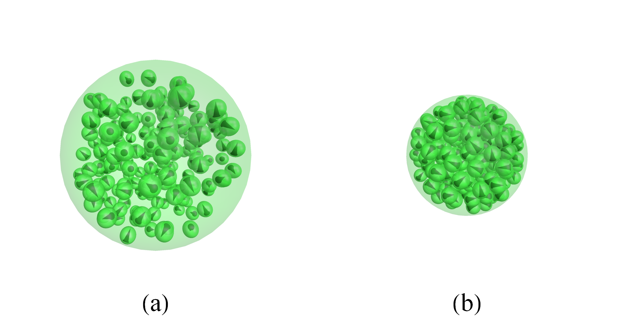
Figure 1: Examples of rigid clusters used in simulations, $\lambda=\sigma=\xi=0$, $N=200$. (a) $\varphi=0.1$, $R\approx 6.3d$, (b) $\varphi=0.3$, $R\approx 4.4d$.

After the cluster is generated, the Heun scheme García-Palacios and Lázaro (1998) is used for the numerical integration of Eq. (33) the damping constant is $\alpha=0.2$, the integration time step is $\Delta t^{*}=0.002$, unless otherwise specified. Dipole-dipole interaction fields between particles in the cluster are calculated without truncation, no periodic boundary conditions (PBCs) are applied. The main result of the simulation is the average normalized magnetization of the cluster $\langle m_{h}\rangle$. In the case $\sigma=0$, the sampling of $m_{h}$ values typically starts after the time $t^{*}=100$, but for $\sigma>0$ a much longer equilibration period might be required. This issue is discussed in Sec. III.3. For each particular set of input parameters, the magnetization value is additionally averaged over several independent realizations of the cluster. However, the results for different realizations are proved to be close, so their number is not large. Most of the magnetization curves presented below are averaged over ten realizations of the cluster.

In addition to clusters, this paper also briefly discusses the equilibrium magnetization of a bulk solid dispersion of magnetic nanoparticles (see Sec. III.1). The input simulation parameters in this case are the same as for the cluster. The simulation cell is a cube with a side length of $L=d\sqrt[3]{\pi N/6\varphi}$. PBCs are applied in all three directions. The dipolar fields in the system are calculated using the standard Ewald summation with “metallic” boundary conditions. This technique ensures a proper handling of long-range effects of dipole-dipole interactions. In its “metallic” version the internal field in the simulation box coincides exactly with the applied field. A detailed description of the technique is available in Refs. Wang et al. (2002); Wang and Holm (2001).

III Results and discussion

III.1 Magnetically isotropic particles in a bulk solid matrix

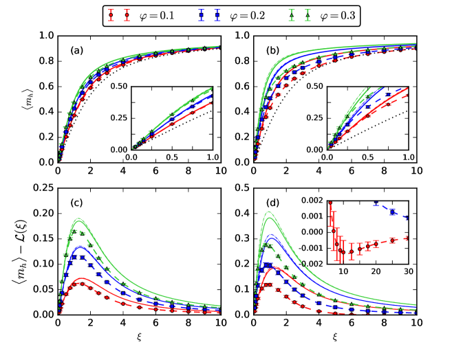
Figure 2: Equilibrium magnetization curves of bulk solid systems with $H=H_{int}$ and $\sigma=0$. $\lambda=1$ (a) and $3$ (b). Symbols are the simulation results for $N=1000$, different combinations of symbols and colors correspond to different particle volume fractions $\varphi$ (see legend). Solid curves are MMFT1 results for the same values of $\varphi$ [Eqs. (25) and (26)], dot-dashed lines are MMFT2 results [Eqs. (25) and (27)], dashed curves are from the analytical model given by Eqs. (25) and (39), dotted lines are from the Langevin model [Eq. (14)]. Insets in (a) and (b) zoom on the weak field region. Figures (c) and (d) show differences between the magnetization values shown in (a), (b) and the Langevin function; (c) corresponds to (a) (i.e., to $\lambda=1$) and (d) corresponds to (b) (i.e., to $\lambda=3$). The inset in (d) shows values of $\langle m_{h}\rangle-{\cal L}(\xi)$ in the strong field region.

Before moving on to the main object of our interest, i.e. the finite-size magnetic cluster, it may be useful to consider the equilibrium magnetization of a bulk solid matrix filled with magnetic nanoparticles and to test the applicability of MMFTs for such system. In numerical simulations we model bulk in a standard way by applying PBCs to a cubic simulation cell. First of all, the usage of PBCs minimizes possible size effects that may arise in the simulation of the cluster. Besides, we use the “metallic” version of the Ewald summation technique to calculate dipole-dipole interactions. This method assumes that the large system formed by the simulation cell and its PBC-images is surrounded by a medium with infinite magnetic permeability Wang et al. (2002). In this case, $\xi=\xi_{int}$ and the system magnetic behavior is the same as that of an elongated cylindrical sample. So, the demagnetizing fields, which are inevitable for the quasi-spherical cluster in a non-magnetic medium, are now absent. In this section, we only consider the case $\sigma=0$.

Static magnetization curves of bulk systems with different values of $\varphi$ and $\lambda$ are given in Fig. 2. To emphasize the effect of interparticle interactions on the equilibrium magnetic properties, we also give in Figs. 2(c) and 2(d) the differences between the system actual magnetization and the Langevin function. Symbols denote values obtained after averaging over ten independent realizations of the simulated system, error bars here and below denote corresponding 95% confidence intervals. It is seen that MMFT1 [Eqs. (25) and (26)] and MMFT2 [Eqs. (25) and (27)] give good agreement with the simulation data in the weak field range ($\xi<1$). In Fig. 3 the system initial susceptibility $\chi$ is plotted vs. the Langevin susceptibility $\chi_{L}$.

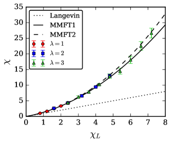
Figure 3: Initial magnetic susceptibility $\chi$ of magnetoisotropic particles embedded in a bulk solid matrix vs. the Langevin susceptibility $\chi_{L}$. Symbols are the simulation results for $N=1000$, different symbols correspond to different values of the dipolar coupling constant $\lambda$ (see legend). Dotted line corresponds to the Langevin model ($\chi=\chi_{L}$), solid line is from MMFT1 [Eq. (36)], dashed line is from MMFT2 [Eq. (37)].

According to MMFT1, the susceptibility is Ivanov and Kuznetsova (2001)

$$\chi=\chi_{L}(1+\chi_{L}/3),$$ (36)

and according to MMFT2, it is

$$\chi=\chi_{L}(1+\chi_{L}/3+\chi_{L}^{2}/144).$$ (37)

The susceptibility of the simulated system is estimated simply as $\chi=3\chi_{L}\langle m_{h}(\xi=0.05)\rangle/0.05$. For $\lambda\leq 3$ and $\varphi\leq 0.25$, MMFT1 describes calculated susceptibilities well, which agrees with the results of Ref. Wang et al. (2002). At $\lambda=3$ and $\varphi>0.25$ (which corresponds to $\chi_{L}>6$ for $\lambda=3$), the susceptibility is seemingly better described by MMFT2. In Ref. Wang et al. (2002) the behavior of solid systems at $\varphi>0.25$ was not investigated. More conspicuous deviations between MMFT1 and the simulation results are observed in Fig. 2 at moderate and strong fields. The theory clearly overestimates the simulation results at $\xi\geq 1$ for all inspected values of interaction parameters. The deviation is larger for higher $\lambda$. As seen in Figs. 2(c) and 2(d), the magnetization of a bulk solid system at moderate and large $\xi$ is closer to the Langevin curve than MMFT1 predicts. Despite this fact, the deviation between the simulation results and the Langevin model is still significant. The maximum difference between $\langle m_{h}\rangle$ and ${\cal L}(\xi)$ is observed at $\xi\sim 1$. For $\lambda=3$ and $\varphi=0.3$, it reaches $\approx 0.28$. In other words, the difference between the non-reduced magnetization $M$ and $M_{L}$ is $\approx 28\%$ of the system saturation magnetization $M_{\infty}$. As $\xi$ increases, the calculated magnetization approaches the Langevin curve much faster than it should according to MMFT1. For one of the investigated parameter sets ($\lambda=3$, $\varphi=0.1$), the calculated values of $\langle m_{h}\rangle$ are even smaller than ${\cal L}(\xi)$ at $\xi\gtrsim 7$ (though the maximum value of the difference $M_{L}-M$ is less than one percent of $M_{\infty}$ as seen in the inset of Fig. 2(d)). As for MMFT2, it overestimates simulation data at large fields even stronger than MMFT1. Such overestimation was not observed in ferrofluid simulations – in the strong coupling case ($\lambda>2$) and at $\xi\geq 1$ the ferrofluid magnetization is either slightly lower than predictions of MMFTs (at high concentrations) or greatly exceeds it (at low concentrations) Wang et al. (2002). A possible explanation is as follows. According to MMFTs, the effective field $H_{eff}$ acting on an arbitrary particle $i$ is always larger than the applied field $H$ and the difference $H_{eff}-H$ becomes larger with increasing $H$. Within this theory, dipole-dipole interactions between the $i$th particle and its surroundings, on average, always help the particle to align with the applied field. Based on our simulation results, this is true for solid dispersions of magnetic particles in the weak field limit. But at large fields the situation can become complicated due to the anisotropic nature of dipole-dipole interactions. Let us choose a Cartesian coordinate system so that its center coincides with the center of the $i$th particle and the $Z$ axis coincides with the applied field direction $\bm{h}$. If $\xi$ is large enough, magnetic moments of all particles in the system are predominantly directed along the $Z$ axis. If the particle $j$ with $\bm{e}_{j}||\bm{h}$ is placed somewhere on the $Z$ axis, then the dipolar field created by this particle at the location of the $i$th particle is co-directed with $\bm{h}$. However, if the $j$th particle is placed in the $XY$ plane, then its dipolar field at the $i$th particle location is directed opposite to $\bm{h}$. In ferrofluids, the anisotropy of dipole-dipole interactions results in the field-induced anisotropy of the pair distribution functionElfimova et al. (2012). In a liquid matrix, the probability to find the $j$th particle on the $Z$ axis in the close contact with the particle $i$ becomes higher with increasing $\xi$. Two co-directed particles with $\bm{r}_{ij}||\bm{h}$ tend to attract each other and form an energetically favorable “head-to-tail” configuration. This effect is noticeable even at relatively low dipolar coupling $\lambda\simeq 1$. At large $\lambda$, it transforms in the well-known formation of chain-like aggregates. On the contrary, the probability to find the $j$th particle in the plane $XY$ in the close contact with the particle $i$ decreases with increasing $\xi$. Two co-directed particles with $\bm{r}_{ij}\perp\bm{h}$ tend to repel each other. So, as the field increases, magnetic particles in a liquid matrix tend to redistribute themselves so that the local surroundings of the $i$th particle is more likely to contain particles that favor the orientation of $\bm{e}_{i}$ along $\bm{h}$. But in our case, the isotropic spatial distribution of particles is frozen. So, at large applied fields the $i$th particle is surrounded both by particles that help it to align with the field and by particles that interfere with such behavior. It seems probable that, as the average result of such competition, the effective field $H_{eff}$ acting on the $i$th particle in a solid matrix with increasing $H$ becomes smaller than the corresponding effective field in a liquid matrix. As the inset in Fig. 2(d) suggests, in some cases $H_{eff}$ can even become slightly smaller than $H$. In Eq. (25) the effect of the particle surroundings is controlled by the mean-field parameter ${\cal C}_{mf}$. In order to correctly describe the observed behavior of a solid dispersion, this parameter should become significantly lower than the standard MMFT1 value $\chi_{L}$ at large fields.

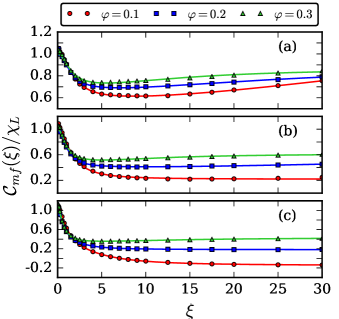
Figure 4: Applied field dependencies of the mean-field parameter for bulk solid systems of magnetoisotropic particles. $\lambda=1$ (a), 2 (b) and 3 (c). Symbols are simulation results for $N=1000$, different symbols correspond to different volume fractions (see legend). Solid lines are from the approximation Eq. (39).

Figure 4 shows the values of ${\cal C}_{mf}$ extracted from the simulation data using the expression

$${\cal C}_{mf}(\xi)=\frac{{\cal L}^{-1}\big{(}\langle m_{h}\rangle\big{)}-\xi}{{\cal L}(\xi)},$$ (38)

where ${\cal L}^{-1}(x)$ is the inverse Langevin function (its values where obtained numerically). The mean-field parameter in the figure is dived by $\chi_{L}$. It is seen that at $\xi\ll 1$ ${\cal C}_{mf}/\chi_{L}\gtrsim 1$, but it becomes lower at large fields, just as expected. At $\xi\lesssim 2$, values of ${\cal C}_{mf}/\chi_{L}$ decrease relatively fast, at a given $\lambda$ they are almost the same for different volume fractions. For $\xi>2$, the quantity ${\cal C}_{mf}/\chi_{L}$ seemingly begins to reach a plateau. The values of ${\cal C}_{mf}/\chi_{L}$ at large fields for different combinations of $\lambda$ and $\varphi$ do not coincide. Particularly, they are very different for $\lambda=1$ and $\varphi=0.3$ and for $\lambda=3$ and $\varphi=0.1$, despite the fact that the Langevin susceptibility is the same in both cases ($\chi_{L}=2.4$). For $\lambda=3$ and $\varphi=0.1$, the mean-field parameter at large $\xi$ becomes negative, which is why $\langle m_{h}\rangle$ at these parameters becomes smaller than ${\cal L}(\xi)$. At large $\xi$, values of ${\cal C}_{mf}/\chi_{L}$ increase with increasing $\varphi$ if $\lambda$ is fixed. The increase in $\lambda$ at a fixed volume fraction has the opposite effect – in this case ${\cal C}_{mf}/\chi_{L}$ decreases. To be able to check whether or not the mean-field parameters obtained for bulk systems are applicable for the description of clusters at large fields, we approximated the dependencies presented in Fig. 4 with the expression

$${\cal C}_{mf}(\xi)=\chi_{L}\frac{1+a_{2}\xi^{2}+a_{4}\xi^{4}}{1+b_{2}\xi^{2}+b_{4}\xi^{4}}.$$ (39)

Eq. (39) contains only even powers of $\xi$, so that Eq. (25) remains an odd function of the magnetic field. Coefficients $a_{2}$, $a_{4}$, $b_{2}$ and $b_{4}$ were separately determined for each investigated combination of $\lambda$ and $\varphi$ using non-linear least squares fitting. The calculated values are given in Table 1. The approximations are valid at least up to $\xi=30$.

Table 1: Fitting parameters of Eq. (39) for different dipolar coupling constants and particle volume fractions.

$\lambda$	$\varphi$	$a_{2}$	$a_{4}$	$b_{2}$	$b_{4}$
1	0.1	0.165553	0.000119	0.286021	0.000083
	0.2	0.294838	0.000583	0.444823	0.000662
	0.3	0.289164	0.001879	0.417613	0.002166
2	0.1	0.312283	0.015637	0.629365	0.071964
	0.2	0.340067	0.000143	0.854058	0.000202
	0.3	0.429252	0.004477	0.901514	0.007247
3	0.1	0.217007	-0.004704	0.864708	0.031570
	0.2	1.632664	0.128207	3.249253	0.708223
	0.3	0.555831	0.004696	1.689059	0.010885

III.2 Cluster of magnetically isotropic particles

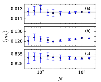
Figure 5: Normalized equilibrium magnetization of the cluster vs. the number of particles it contains. $\lambda=3$, $\varphi=0.3$ and $\sigma=0$. $\xi=0.1$ (a), 1 (b), 10 (c). Symbols are simulation results. Horizontal lines correspond to predictions of the analytical model given by Eqs. (28) and (39).

One of our main concerns regarding simulations of the cluster were possible finite-size effects. In Ref. Wang et al. (2003) it was shown that properties of finite spherical containers with ferrofluid depend heavily on the system size in the case of strong dipolar coupling. Equilibrium magnetization of systems with $N\sim 10^{2}$–$10^{3}$ proved to be much smaller than corresponding thermodynamic limit values. Magnetization values of rigid clusters with $\sigma=0$ are shown in Fig. 5 as a function of the particle number $N$ at different values of $\xi$. These data are calculated for $\lambda=3$ and $\varphi=0.3$, i.e. for the largest values of interaction parameters considered in this work. Luckily, the results do not indicate strong size dependencies for rigid quasi-spherical clusters. This gives hope that approximations Eq. (39) derived for a bulk system will work for small clusters as well.

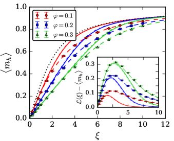
Figure 6: Equilibrium magnetization curves of clusters with $\sigma=0$ and $\lambda=3$. Symbols are simulation results for $N=1000$, different combinations of symbols and colors correspond to different volume fractions (see legend). Solid cures are prediction of MMFT1 [Eqs. (26) and (28)] for the same volume fractions, dot-dashed curves are predictions of MMFT2 [Eqs. (27) and (28)]. Dashed lines are from the analytical model given by Eqs. (28) and (39). Dotted line is the Langevin function [Eq. (14)]. The inset shows corresponding differences between the Langevin function and magnetization values.

Static magnetization curves for clusters with $\sigma=0$ and $\lambda=3$ are given in Fig. 6. Due to the presence of demagnetizing fields, the effect of interactions is the opposite of what was observed in the previous section. Magnetization of the cluster is now always smaller than the Langevin model predicts and the cluster equilibrium response is weaker the higher the volume fraction $\varphi$. Just like in the bulk case, MMFT1 (which is now given by Eqs. (26) and (28)) provides an accurate description of the magnetization curve initial slope, but overestimates the simulation results at strong fields ($\xi\gtrsim 2$). MMFT2 [Eqs. (27) and (28)] again gives larger magnetization values than MMFT1, but it should be noted that the difference between two theories is much less pronounced than in the bulk case. The combination of Eq. (28) and approximation Eq. (39) with fitting parameters taken from Table 1 accurately describes the cluster magnetization at all investigated values of $\varphi$ and $\xi$. The foregoing is also true for smaller coupling parameters, but the difference between the cluster magnetization and the Langevin function in this case is much less distinguishable. For example, at $\lambda=1$ and $\varphi=0.3$, the maximum value of ${\cal L}(\xi)-\langle m_{h}\rangle$ is $\approx 0.09$. For $\lambda=3$ and $\varphi=0.3$, the difference ${\cal L}(\xi)-\langle m_{h}\rangle$ can become larger than $0.3$ (which is seen in the inset of Fig. 6).

III.3 Cluster of uniaxial particles

Figure 7: Instantaneous values of the cluster normalized magnetization vs. simulation time. Simulation results for $N=400$, $\lambda=1$, $\varphi=0.1$ and $\xi=1$. From top to bottom: $\sigma=0$, 10, 15 and 20.

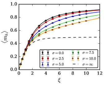
Figure 8: Equilibrium magnetization curves of clusters of non-interacting ($\lambda=0$) uniaxial particles. Symbols are simulation results for $N=400$, different combinations of symbols and colors correspond to different anisotropy parameters $\sigma$ (see legend). Lines are predictions of Eq. (18) for the same values of $\sigma$.

One can expect that the time necessary for the cluster to reach the equilibrium magnetization value from the initial random state will increase with increasing anisotropy parameter $\sigma$. The reason is that magnetic moments of particles will have to overcome the anisotropy energy barrier. In zero magnetic field and in the absence of interactions, the characteristic time scale that determines how long it will take for the magnetic moment to overcome the barrier (i.e., to spontaneously change its orientation from $\bm{n}$ to energetically equivalent $-\bm{n}$) is called the Néel relaxation time ($\tau_{N}$). This time increases exponentially with increasing $\sigma$. With a good accuracy $\tau_{N}$ is given by the approximation Coffey et al. (1994)

$$\tau_{N}=\tau_{D}\frac{e^{\sigma}-1}{2\sigma}\left[\frac{1}{1+1/\sigma}\sqrt{\frac{\sigma}{\pi}}+2^{-\sigma-1}\right]^{-1}.$$ (40)

In the limit of negligible anisotropy ($\sigma\ll 1$), the Néel time $\tau_{N}$ reduces to the relaxation time $\tau_{D}$. Eq. (40) gives $\tau_{N}\simeq 14\tau_{D}$ for $\sigma=5$, $\tau_{N}\simeq 6.8\times 10^{2}\tau_{D}$ for $\sigma=10$, $\tau_{N}\simeq 5.3\times 10^{4}\tau_{D}$ for $\sigma=15$ and $\tau_{N}\simeq 5.0\times 10^{6}\tau_{D}$ for $\sigma=20$. Figure 7 demonstrates a very similar non-linear slow down. This figure shows the dynamics of the cluster magnetization for different values of $\sigma$ at a fixed field $\xi=1$. In the beginning $m_{h}$ is close to zero, but then it starts to increase and gradually reaches a non-zero equilibrium value. It is seen that as $\sigma$ varies from 0 to 20, the characteristic equilibration period increases by several orders of magnitude. For larger fields ($\xi>1$), the period decreases, but the direct simulation of clusters with $\sigma>10$ still remains challenging from a computational viewpoint. Due to the restrictions of available computational resources, only cluster with $N=400$ and $\sigma\leq 10$ are considered below. The integration time step is slightly increased to $\Delta t^{*}=0.003$. Further increase of the time step can potentially lead to erroneous simulation results Ilg (2017). We use equilibration period $t^{*}=500$ for $2.5\leq\sigma\leq 7.5$ and $t^{*}=4000$ for $\sigma=10$.

Magnetization curves of a cluster of non-interacting uniaxial particles ($\lambda=0$) were first calculated as a test. The results are given in Fig. 8. Calculations are in full agreement with Eq. (18). The linear response at weak fields is always the same as for the Langevin model, but for $\xi>1$ the growth of $\langle m_{h}\rangle$ is slower the higher the anisotropy parameter $\sigma$.

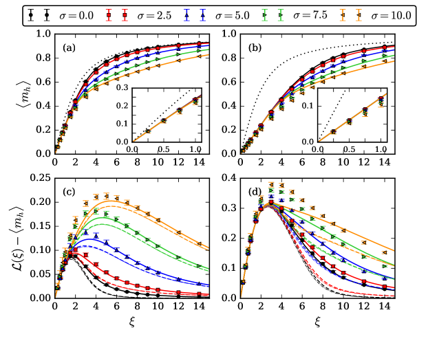
Figure 9: Equilibrium magnetization curves of clusters with $\varphi=0.3$. $\lambda=1$ (a) and $3$ (b). Symbols are the simulation results for $N=400$, different combinations of symbols and colors correspond to different anisotropy parameters $\sigma$ (see legend). Solid curves are predictions of the analytical model given by Eqs. (30) and (39) for the same values of $\sigma$. Dotted lines are from the Langevin model Eq. (14). Insets in (a) and (b) zoom on the weak field region. Figures (c) and (d) show differences between the Langevin function and the magnetization values shown in (a) and (b); (c) corresponds to (a) (i.e., to $\lambda=1$) and (d) corresponds to (b) (i.e., to $\lambda=3$). Dashed lines in (c) and (d) correspond to the analytical model given by Eqs. (26) and (30), dot-dashed lines correspond to the analytical model given by Eqs. (30) and (41).

Magnetization curves for clusters with $\sigma\leq 10$, $\varphi=0.3$ and different values of $\lambda$ are given in Fig. 9. The most noticeable effect of increasing anisotropy, just as in the case of non-interacting particles, is the saturation slowdown at large fields. Our phenomenological modification of MMFT given by Eq. (30) correctly reproduces this feature. As a mean-field parameter in Eq. (30), we use approximation Eq. (39) with fitting parameters previously obtained for bulk magnetoisotropic systems (see Table 1). For $\lambda=1$ (Figs. 9(a) and 9(c)), the combination of Eqs. (30) and (39) shows great quantitative agreement with simulation data. The largest deviations are observed at intermediate fields $2\lesssim\xi\lesssim 6$, where the analytical model overestimates the magnetization of simulated clusters. For $\sigma=10$, the largest deviation is $\approx 0.03$. Deviations become more pronounced at $\lambda=3$ (Figs. 9(b) and 9(d)). At $\sigma=10$, the largest deviation is now $\approx 0.07$. Besides, at $\lambda=3$ and $\xi\gtrsim 10$, calculated magnetizations become larger than predictions of the analytical model. Figs. 9(c) and 9(d) additionally demonstrate the predictions of “anisotropic generalizations” of MMFT1 and MMFT2. For MMFT1, this is simply a combination of Eqs. (26) and (30). For MMFT2, the mean-field parameter Eq. (27) was modified using the same intuitive approach, which was used to obtain Eq. (30) – the function ${\cal L}(\xi)$ was replaced with ${\cal L}_{ani}(\xi,\sigma)$:

$${\cal C}_{mf}(\xi,\sigma)=\chi_{L}\left(1+\frac{\chi_{L}}{16}\frac{\partial{\cal L}_{ani}(\xi,\sigma)}{\partial\xi}\right).$$ (41)

It is seen that “generalized” MMFTs overestimate calculated magnetizations at all field values starting from $\xi\simeq 2$. Just like in Sec. III.2, the predictions of MMFT2 only slightly exceed the predictions of MMFT1.

IV Conclusions

In this work, equilibrium magnetization curves of a random quasi-spherical cluster of single-domain nanoparticles are studied numerically and analytically. Langevin dynamics simulations show that, due to dipole-dipole interactions between particles, magnetization of the cluster is generally lower than predicted by the classical Langevin model. This is in full agreement with recent findings of Refs. Schaller et al. (2009a); Ilg (2017). It is shown that, in the case of negligible magnetic anisotropy and weak applied fields, magnetization curves can be successfully described by the so-called modified mean-field theory, initially proposed for the description of concentrated ferrofluids. However, as the field increases, the theory starts to overestimate the cluster magnetization. The discrepancy can be minimized by adjusting the mean-field parameter of MMFT, so that it decreases with increasing applied field. The explicit form of the dependency between the mean-field parameter ${\cal C}_{mf}$ and the Langevin parameter $\xi$ (which determines the impact of the applied field on the system) is turned out to be different for different values of the dipolar coupling parameter $\lambda$ and the particle volume fraction $\varphi$. For some specific combinations of $\lambda$ and $\varphi$, dependencies ${\cal C}_{mf}={\cal C}_{mf}(\xi)$ are obtained in the form of approximation formulas. Clearly, finding a universal dependency ${\cal C}_{mf}={\cal C}_{mf}(\xi,\lambda,\varphi)$ would be useful from a practical point of view, but this requires a rigorous statistical mechanical treatment of the problem, which is beyond the scope of this work.

It is also shown that if particles have non-negligible anisotropy (characterized by the anisotropy parameter $\sigma$) and the distribution of their easy axes is random and uniform, then, at given values of $\xi$, $\lambda$ and $\varphi$, the magnetization of the cluster decreases with increasing $\sigma$. The decrease is much stronger at large fields. For weak dipolar coupling ($\lambda\simeq 1$), this effect can be accurately taken into account simply by replacing all Langevin functions ${\cal L}(\xi)$ in the magnetization expression given by MMFT [Eq. (28)] with its generalization ${\cal L}_{ani}(\xi,\sigma)$ [Eq. (18)]. Function ${\cal L}_{ani}(\xi,\sigma)$ is the exact solution for magnetization of non-interacting uniaxial particles with random orientation texture. At larger coupling parameters ($\lambda>1$), such simple approach demonstrates noticeable quantitative deviations from the simulation results.

In this work, only monodisperse systems are considered. But it is known that magnetization of rigid clusters can also be influenced by the polydispersity of particles Schaller et al. (2009a). The combined effect of magnetic anisotropy, interparticle interactions and polydispersity on static magnetization curves of finite-size quasi-spherical clusters will be considered in future papers.

V Acknowledgments

The work was supported by Russian Science Foundation (project No. 17-72-10033). The author is grateful to Prof. A. F. Pshenichnikov for valuable discussions.

References

- Gijs (2004) M. A. M. Gijs, “Magnetic bead handling on-chip: new opportunities for analytical applications,” Microfluid. Nanofluid. 1, 22–40 (2004).
- Gervald et al. (2010) A. Yu. Gervald, I. A. Gritskova, and N. I. Prokopov, “Synthesis of magnetic polymeric microspheres,” Russ. Chem. Rev. 79, 219 (2010).
- McCloskey et al. (2003) Kara E. McCloskey, Jeffrey J. Chalmers, and Maciej Zborowski, “Magnetic cell separation: characterization of magnetophoretic mobility,” Anal. Chem. 75, 6868–6874 (2003).
- Leong et al. (2016) Sim Siong Leong, Swee Pin Yeap, and JitKang Lim, “Working principle and application of magnetic separation for biomedical diagnostic at high-and low-field gradients,” Interface focus 6, 20160048 (2016).
- Widder et al. (1978) Kenneth J. Widder, Andrew E. Senyei, and Dante G. Scarpelli, “Magnetic microspheres: a model system for site specific drug delivery in vivo,” Proc. Soc. Exp. Biol. Med. 158, 141–146 (1978).
- Dutz et al. (2012) Silvio Dutz, M. E. Hayden, Allison Schaap, Boris Stoeber, and Urs O. Häfeli, “A microfluidic spiral for size-dependent fractionation of magnetic microspheres,” J. Magn. Magn. Mater. 324, 3791–3798 (2012).
- Amblard et al. (1996) François Amblard, Bernard Yurke, Andrew Pargellis, and Stanislas Leibler, “A magnetic manipulator for studying local rheology and micromechanical properties of biological systems,” Rev. Sci. Instrum. 67, 818–827 (1996).
- van Oene et al. (2015) Maarten M. van Oene, Laura E. Dickinson, Francesco Pedaci, Mariana Köber, David Dulin, Jan Lipfert, and Nynke H. Dekker, “Biological magnetometry: torque on superparamagnetic beads in magnetic fields,” Phys. Rev. Lett. 114, 218301 (2015).
- Yang et al. (2005) Chunqiang Yang, Gang Wang, Ziyang Lu, Jing Sun, Jiaqi Zhuang, and Wensheng Yang, “Effect of ultrasonic treatment on dispersibility of Fe3O4 nanoparticles and synthesis of multi-core Fe3O4/SiO2 core/shell nanoparticles,” J. Mater. Chem. 15, 4252–4257 (2005).
- Dutz et al. (2009) Silvio Dutz, Joachim H. Clement, Dietmar Eberbeck, Thorsten Gelbrich, Rudolf Hergt, Robert Müller, Jana Wotschadlo, and Matthias Zeisberger, “Ferrofluids of magnetic multicore nanoparticles for biomedical applications,” J. Magn. Magn. Mater. 321, 1501–1504 (2009).
- Schaller et al. (2009a) Vincent Schaller, Göran Wahnström, Anke Sanz-Velasco, Peter Enoksson, and Christer Johansson, “Monte carlo simulation of magnetic multi-core nanoparticles,” J. Magn. Magn. Mater. 321, 1400–1403 (2009a).
- Dutz (2016) Silvio Dutz, “Are magnetic multicore nanoparticles promising candidates for biomedical applications?” IEEE Trans. Magn. 52, 1–3 (2016).
- Xu et al. (2011) Hengyi Xu, Zoraida P. Aguilar, Lily Yang, Min Kuang, Hongwei Duan, Yonghua Xiong, Hua Wei, and Andrew Wang, “Antibody conjugated magnetic iron oxide nanoparticles for cancer cell separation in fresh whole blood,” Biomaterials 32, 9758–9765 (2011).
- Dutz et al. (2011) Silvio Dutz, Melanie Kettering, Ingrid Hilger, Robert Müller, and Matthias Zeisberger, “Magnetic multicore nanoparticles for hyperthermia – influence of particle immobilization in tumour tissue on magnetic properties,” Nanotechnology 22, 265102 (2011).
- Blanco-Andujar et al. (2015) C. Blanco-Andujar, D. Ortega, P. Southern, Q. A. Pankhurst, and N. T. K. Thanh, “High performance multi-core iron oxide nanoparticles for magnetic hyperthermia: microwave synthesis, and the role of core-to-core interactions,” Nanoscale 7, 1768–1775 (2015).
- Lartigue et al. (2012) Lénaic Lartigue, Pierre Hugounenq, Damien Alloyeau, Sarah P Clarke, Michael Lévy, Jean-Claude Bacri, Rana Bazzi, Dermot F. Brougham, Claire Wilhelm, and Florence Gazeau, “Cooperative organization in iron oxide multi-core nanoparticles potentiates their efficiency as heating mediators and MRI contrast agents,” ACS nano 6, 10935–10949 (2012).
- Eberbeck et al. (2013) Dietmar Eberbeck, Cindi L. Dennis, Natalie F. Huls, Kathryn L. Krycka, Cordula Gruttner, and Fritz Westphal, “Multicore magnetic nanoparticles for magnetic particle imaging,” IEEE Transactions on Magnetics 49, 269–274 (2013).
- Buzmakov and Pshenichnikov (1996) V. M. Buzmakov and A. F. Pshenichnikov, “On the structure of microaggregates in magnetite colloids,” J. Colloid Interface Sci. 182, 63–70 (1996).
- Magnet et al. (2012) Cécilia Magnet, Pavel Kuzhir, Georges Bossis, Alain Meunier, Liudmila Suloeva, and Andrey Zubarev, “Haloing in bimodal magnetic colloids: The role of field-induced phase separation,” Phys. Rev. E 86, 011404 (2012).
- Ivanov and Pshenichnikov (2010) A. S. Ivanov and A. F. Pshenichnikov, “Magnetophoresis and diffusion of colloidal particles in a thin layer of magnetic fluids,” J. Magn. Magn. Mater. 322, 2575–2580 (2010).
- Borin et al. (2011) Dmitry Borin, Andrey Zubarev, Dmitry Chirikov, Robert Müller, and Stefan Odenbach, “Ferrofluid with clustered iron nanoparticles: Slow relaxation of rheological properties under joint action of shear flow and magnetic field,” J. Magn. Magn. Mater. 323, 1273–1277 (2011).
- Guo et al. (2003) Zheng Guo, Shu Bai, and Yan Sun, “Preparation and characterization of immobilized lipase on magnetic hydrophobic microspheres,” Enzyme Microb. Technol. 32, 776–782 (2003).
- Schaller et al. (2009b) Vincent Schaller, Göran Wahnström, Anke Sanz-Velasco, Stefan Gustafsson, Eva Olsson, Peter Enoksson, and Christer Johansson, “Effective magnetic moment of magnetic multicore nanoparticles,” Phys. Rev. B 80, 092406 (2009b).
- Usov and Serebryakova (2016) N. A. Usov and O. N. Serebryakova, “Universal behavior of dense clusters of magnetic nanoparticles,” AIP Adv. 6, 075315 (2016).
- Ilg (2017) Patrick Ilg, “Equilibrium magnetization and magnetization relaxation of multicore magnetic nanoparticles,” Phys. Rev. B 95, 214427 (2017).
- Weddemann et al. (2010) Alexander Weddemann, Alexander Auge, D. Kappe, Frank Wittbracht, and Andreas Hütten, “Dynamic simulations of the dipolar driven demagnetization process of magnetic multi-core nanoparticles,” J. Magn. Magn. Mater. 322, 643–646 (2010).
- Melenev et al. (2010) P. V. Melenev, R. Perzynski, Yu. L. Raikher, and V. V. Rusakov, “Monte carlo model for the dynamic magnetization of microspheres,” Physics Procedia 9, 54–57 (2010).
- Usov et al. (2017) N. A. Usov, O. N. Serebryakova, and V. P. Tarasov, “Interaction effects in assembly of magnetic nanoparticles,” Nanoscale Res. Lett. 12, 489 (2017).
- Huke and Lücke (2004) B Huke and M Lücke, “Magnetic properties of colloidal suspensions of interacting magnetic particles,” Rep. Prog. Phys. 67, 1731 (2004).
- Pshenichnikov et al. (1996) A. F. Pshenichnikov, V. V. Mekhonoshin, and A. V. Lebedev, “Magneto-granulometric analysis of concentrated ferrocolloids,” J. Magn. Magn. Mater. 161, 94–102 (1996).
- Ivanov and Kuznetsova (2001) Alexey O. Ivanov and Olga B. Kuznetsova, “Magnetic properties of dense ferrofluids: an influence of interparticle correlations,” Phys. Rev. E 64, 041405 (2001).
- Ivanov et al. (2007) Alexey O. Ivanov, Sofia S. Kantorovich, Evgeniy N. Reznikov, Christian Holm, Alexander F. Pshenichnikov, Alexander V. Lebedev, Alexandros Chremos, and Philip J. Camp, “Magnetic properties of polydisperse ferrofluids: A critical comparison between experiment, theory, and computer simulation,” Phys. Rev. E 75, 061405 (2007).
- Wang et al. (2002) Zuowei Wang, Christian Holm, and Hanns Walter Müller, “Molecular dynamics study on the equilibrium magnetization properties and structure of ferrofluids,” Phys. Rev. E 66, 021405 (2002).
- Pshenichnikov and Mekhonoshin (2000) A. F. Pshenichnikov and V. V. Mekhonoshin, “Equilibrium magnetization and microstructure of the system of superparamagnetic interacting particles: numerical simulation,” J. Magn. Magn. Mater. 213, 357–369 (2000).
- Rosensweig (2002) R. E. Rosensweig, “Heating magnetic fluid with alternating magnetic field,” J. Magn. Magn. Mater. 252, 370–374 (2002).
- Bean and Livingston (1959) C. P. Bean and J. D. Livingston, “Superparamagnetism,” J. Appl. Phys. 30, S120–S129 (1959).
- Raikher (1983) Yu. L. Raikher, “The magnetization curve of a textured ferrofluid,” J. Magn. Magn. Mater. 39, 11–13 (1983).
- Chantrell et al. (1985) R. W. Chantrell, N. Y. Ayoub, and J. Popplewell, “The low field susceptibility of a textured superparamagnetic system,” J. Magn. Magn. Mater. 53, 199–207 (1985).
- Williams et al. (1993) H. D. Williams, K. O’Grady, M. El Hilo, and R. W. Chantrell, “Superparamagnetism in fine particle dispersions,” J. Magn. Magn. Mater. 122, 129–133 (1993).
- Mamiya and Nakatani (1998) H. Mamiya and I. Nakatani, “Magnetization curve for iron-nitride fine particle system with random anisotropy,” IEEE Trans. Magn. 34, 1126–1128 (1998).
- Cregg and Bessais (1999) P. J. Cregg and Lotfi Bessais, “Series expansions for the magnetisation of a solid superparamagnetic system of non-interacting particles with anisotropy,” J. Magn. Magn. Mater. 202, 554–564 (1999).
- Joseph and Schlömann (1965) R. I. Joseph and E. Schlömann, “Demagnetizing field in nonellipsoidal bodies,” J. Appl. Phys. 36, 1579–1593 (1965).
- Kittel (2004) C. Kittel, Introduction to solid state physics (Wiley, 2004).
- Tsebers (1982) A. O. Tsebers, “Thermodynamic stability of magnetofluids,” Magnetohydrodynamics 18, 137–142 (1982).
- Zhang and Widom (1995) H. Zhang and M. Widom, “Spontaneous magnetic order in random dipolar solids,” Phys. Rev. B 51, 8951 (1995).
- Wei and Patey (1992) Dongqing Wei and G. N. Patey, “Orientational order in simple dipolar liquids: computer simulation of a ferroelectric nematic phase,” Phys. Rev. Lett. 68, 2043 (1992).
- Klapp and Patey (2001) S. H. L. Klapp and G. N. Patey, “Ferroelectric order in positionally frozen dipolar systems,” J. Chem. Phys. 115, 4718–4731 (2001).
- Ivanov et al. (2004) Alexey O. Ivanov, Zuowei Wang, and Christian Holm, “Applying the chain formation model to magnetic properties of aggregated ferrofluids,” Phys. Rev. E 69, 031206 (2004).
- García-Palacios and Lázaro (1998) José Luis García-Palacios and Francisco J. Lázaro, “Langevin-dynamics study of the dynamical properties of small magnetic particles,” Phys. Rev. B 58, 14937 (1998).
- Wang and Holm (2001) Zuowei Wang and Christian Holm, “Estimate of the cutoff errors in the ewald summation for dipolar systems,” J. Chem. Phys. 115, 6351–6359 (2001).
- Elfimova et al. (2012) Ekaterina A. Elfimova, Alexey O. Ivanov, and Philip J. Camp, “Theory and simulation of anisotropic pair correlations in ferrofluids in magnetic fields,” J. Chem. Phys. 136, 194502 (2012).
- Wang et al. (2003) Zuowei Wang, Christian Holm, and Hanns Walter Müller, “Boundary condition effects in the simulation study of equilibrium properties of magnetic dipolar fluids,” J. Chem. Phys. 119, 379–387 (2003).
- Coffey et al. (1994) W. T. Coffey, P. J. Cregg, D. S. F. Crothers, J. T. Waldron, and A. W. Wickstead, “Simple approximate formulae for the magnetic relaxation time of single domain ferromagnetic particles with uniaxial anisotropy,” J. Magn. Magn. Mater. 131, L301–L303 (1994).