Symmetry enhanced first-order phase transition in a two-dimensional quantum magnet

Abstract

Theoretical studies of quantum phase transitions have suggested critical points with higher symmetries than those of the underlying Hamiltonian. Here we demonstrate a surprising emergent symmetry of the coexistence state at a strongly discontinuous phase transition between two ordered ground states. We present a quantum Monte Carlo study of a two-dimensional $S=1/2$ quantum magnet hosting the antiferromagnetic (AFM) and plaquette-singlet solid (PSS) states recently detected in SrCu₂(BO₃)₂. We observe that the O(3) symmetric AFM order and the Z₂ symmetric PSS order form an O(4) vector at the transition. The control parameter $g$ (a coupling ratio) rotates the vector between the AFM and PSS sectors and there are no energy barriers between the two at the transition point $g_{c}$. This phenomenon may be observable in SrCu₂(BO₃)₂.

Introduction.—Theoretical studies of exotic quantum states of matter and the phase transitions between them can provide new perspectives on many-body physics and stimulate experimental investigations. A prominent example is the quantum phase transition between antiferromagnetic (AFM) and spontaneously dimerized valence-bond solid (VBS) ground states in two-dimensional (2D) spin $S=1/2$ magnets Sachdev_NPH_2008 ; Kaul_ARC_2012 . Here the theory of deconfined quantum critical points (DQCPs) suggests that the Landau-Ginzburg-Wilson (LGW) paradigm for phase transitions is inapplicable, as a consequence of quasi-particle fractionalization Senthil_Sci_2004 ; Senthil_PRB_2004 . Over the past decade, likely DQCPs have been identified in lattice models, using “designer Hamiltonians” constructed for their amenability to large-scale quantum Monte Carlo (QMC) simulations of the AFM–VBS transition Sandvik_PRL_2007 ; Melko_PRL_2008 ; Jiang_JST_2008 ; Kuklov_PRL_2008 ; Lou_PRB_2009 ; Sandvik_PRL_2010 ; Chen_PRL_2013 ; Harada_PRB_2013 ; Pujari_PRL_2013 ; Block_PRL_2013 ; Nahum_PRX_2015 ; Shao_Sci_2016 . Recently, a potential experimental realization of this type of DQCP was reported in the quasi-2D Shastry-Sutherland (SS) compound SrCu₂(BO₃)₂ under pressure Zayed_NP_2017 . Though the SS model Shastry_Phy_1981 is difficult to study numerically, due to its geometrical frustration (which causes sign problems in QMC simulations), a specific type of VBS—a two-fold degenerate plaquette-singlet solid (PSS) located between AFM and bond-singlet phases—was demonstrated convincingly by tensor-network calculations Corboz_PRB_2013 . Zayed et al. Zayed_NP_2017 showed that a PSS also exists in SrCu₂(BO₃)₂ and suggested that the AFM–PSS transition may be a DQCP. The phase transition was not studied in the experiment, however, and it is not immediately clear if the two-fold degenerate PSS can support spinon deconfinement in the same way as a four-fold degenerate VBS. QMC studies of rectangular lattices with two-fold degenerate VBS states point to a first-order transition Block_PRL_2013 , as was also found in the SS model Corboz_PRB_2013 .

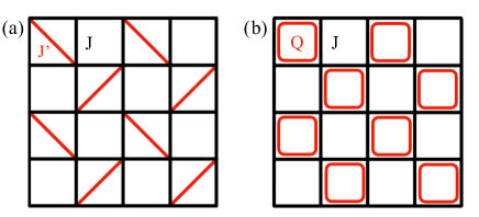
Here we study a sign-free model that mimics the SS compound, in the sense that it shares the same kinds of AFM and PSS ground states. The Hamiltonian, illustrated in Fig. 1 along with the SS model, is a new member in the “$J$-$Q$” family Sandvik_PRL_2007 , with Heisenberg exchange $J$ supplemented by four-spin interactions $Q$ that weaken and eventually destroy the AFM order. Our QMC simulations demonstrate a first-order AFM–PSS transition with emergent O(4) symmetry.

Figure 1: In the SS model (a), Heisenberg exchange $J$ between nearest neighbor $S=1/2$ spins compete with next-nearest neighbor couplings indicated by diagonal lines. In the CBJQ model (b) the $J^{\prime}$ interactions are replaced by the $Q$ terms in Eq. (1).

Non-LGW critical points with emergent symmetries have been extensively investigated recently Nahum_PRL_2015 ; Karch_PRX_2016 ; Metlitski_PRB_2016 ; Mross_PRL_2016 ; Kachru_PRL_2017 ; Wang_PRX_2017 ; Qin_PRX_2017 ; Sato_PRL_2017 ; Metlitski_2017 ; Gazit_2018 ; Stre_2018 . In the case discussed here, the order parameters exhibit clear discontinuities but conventional phase coexistence is not observed. Using order-parameter distributions, we show that the AFM order is rotated by the control parameter into PSS order. Phase coexistence at the transition takes the form of an O(4) symmetric vector arising out of the O(3) AFM and $Z_{2}$ PSS order parameters, with no energy barrier separating the two phases. In further support of this scenario, we demonstrate a characteristic logarithmic form of the PSS ordering temperature versus the tuning parameter, as expected for a 2D O($N\geq 3$) quantum system deformed by a $Z_{2}$ interaction Irkhin_PRB_1998 ; Cuccoli_PRB_2003 .

Ground states.—Our Hamiltonian can be defined using singlet projection operators $P_{ij}=(1/4-{\bf S}_{i}\cdot{\bf S}_{j})$;

$$H=-J\sum_{\langle ij\rangle}P_{ij}-Q\hskip-5.69054pt\sum_{ijkl\in\Box^{\prime}}\hskip-2.84526pt(P_{ij}P_{kl}+P_{ik}P_{jl}),$$ (1)

where all indicated site pairs are nearest neighbors on a periodic square lattice with $L^{2}$ sites and $\Box^{\prime}$ denotes the $2\times 2$ $Q$-plaquettes in Fig. 1(b). We define $g=J/Q$. For $g\to\infty$, this checker-board $J$-$Q$ (CBJQ) model reduces to the usual AFM ordered (at temperature $T=0$) Heisenberg model, and for $g\to 0$ we will demonstrate a two-fold degenerate PSS. The model does not have any phase corresponding to the $J^{\prime}$-bond singlet state of the SS model for large $J^{\prime}/J$. However, for elucidating the nature of the AFM–PSS transition, we can invoke symmetries and universality to propose that the two models, as well as SrCu₂(BO₃)₂, contain the same physics.

We use two different QMC methods to study the CBJQ model: ground-state projection in the basis of valence bonds Sandvik_PRB_2010 and the stochastic series expansion (SSE) method Sandvik_AIP_2010 . Both techniques deliver exact results to within statistical errors. The projector method is very useful for studying spin-rotationally averaged quantities, while the SSE method is more efficient for finite-size scaling when the finite-$L$ ground states do not have to be fully reached but $T\to 0$ as $L\to\infty$.

Figure 2: Dimer order distribution $P(D_{x},D_{y})$ in the ground state of the CBJQ model at $g=0.20$ (in the PSS phase) and at $g=0.24$ (in the AFM phase), from valence-bond QMC on $L=96$ lattices.

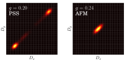
To demonstrate the PSS ground state for large $g$, we first study a conventional dimer order parameter

$$D_{\mu}=\frac{1}{L^{2}}\sum_{\mathbf{r}}(-1)^{r_{\mu}}{\bf S}(\mathbf{r})\cdot{\bf S}(\mathbf{r}+\hat{\mu}),\quad\mu=x,y,$$ (2)

where the sum is over the lattice sites at $\mathbf{r}=(r_{x},r_{y})$. In a VBS, $\langle D_{x}\rangle\not=0,\langle D_{y}\rangle=0$ for $x$-oriented bond order and the same with $x\leftrightarrow y$ for $y$-orientation. Since a singlet plaquette can be regarded as a resonance between horizontal and vertical bond pairs, a two-fold degenerate PSS should have $|\langle D_{x}\rangle|=|\langle D_{y}\rangle|\not=0$ due to modulated singlet density on the plaquette rows and columns in Fig. 1. On a finite lattice the symmetry is not broken, and the system fluctuates between the two states. We use the projector method to generate the probability distribution $P(D_{x},D_{y})$. While strictly not a quantum mechanical observable, this distribution nevertheless properly reflects the fluctuations and symmetries of the system. Results on either side of the AFM–PSS transition (the location of which will be determined below) are shown in Fig. 2. We see the two-fold symmetry of a PSS, instead of the four-fold symmetry of the columnar VBS Lou_PRB_2009 ; Sandvik_PRB_2012 .

If the $Q$ terms are included on all plaquettes we arrive back to the original $J$-$Q$ model, whose AFM–VBS transition appears to be continuous Shao_Sci_2016 . In accord with the DQCP theory, an emergent U(1) symmetry of its microscopically $Z_{4}$ invariant VBS order parameter has been confirmed Sandvik_PRL_2007 ; Jiang_JST_2008 ; Sandvik_PRB_2012 . The proposed field theory description with spinons coupled to an U(1) gauge field Senthil_Sci_2004 ; Senthil_PRB_2004 therefore seems viable. Unusual finite-size scaling behaviors not contained within the theory (but not contradicted by it) have also been observed Sandvik_PRL_2010 ; Nahum_PRX_2015 ; Shao_Sci_2016 (and interpreted by some as a weak first-order transition Kuklov_PRL_2008 ; Jiang_JST_2008 ; Chen_PRL_2013 ). An interesting proposal is that the O(3) symmetry of the AFM and the emergent U(1) symmetry of the VBS may combine into an SO(5) symmetry exactly at the critical point Senthil_PRB_2006 ; Nahum_PRL_2015 . In a spin-planar $J$-$Q$ model, it has instead been demonstrated that the U(1) AFM order parameter and the emergent U(1) VBS symmetry combine into a emergent O(4) symmetry Qin_PRX_2017 . In yet another example, it was proposed that a system with O(3) AFM order and Z₂ Kekule VBS state exhibits a DQCP with emergent SO(4) symmetry Sato_PRL_2017 . The O(3) and $Z_{2}$ symmetries apply also to the CBJQ model, and we therefore pay attention to a potential O(4) or SO(4) symmetry so4note .

Finite-size scaling.—To analyze the AFM–PSS transition, we perform SSE calculations at $T=2/L$. This way of taking the limit $T\to 0,L\to\infty$ is appropriate for a quantum phase transition with dynamic exponent $z=1$, as well as a for a first-order transition. We use order parameters defined solely with the $S^{z}$ spin components,

$$m_{z}=\frac{1}{L^{2}}\sum_{\mathbf{r}}\phi(\mathbf{r})S^{z}(\mathbf{r}),\leavevmode\nobreak\ \leavevmode\nobreak\ m_{p}=\frac{2}{L^{2}}\sum_{\mathbf{q}}\theta(\mathbf{q})\Pi^{z}(\mathbf{q}),$$ (3)

where the subscripts $z$ (spin component) and $p$ (plaquette) mark the AFM and PSS order parameters, respectively. In $m_{z}$, $\mathbf{r}$ runs over all $L^{2}$ lattice sites and $\phi(\mathbf{r})=\pm 1$ is the staggered AFM sign. In $m_{p}$, we have defined an operator

$$\Pi^{z}(\mathbf{q})=S^{z}(\mathbf{q})S^{z}(\mathbf{q}+\hat{x})S^{z}(\mathbf{q}+\hat{y})S^{z}(\mathbf{q}+\hat{x}+\hat{y}),$$ (4)

for detecting plaquette modulation, and the index $\mathbf{q}$ runs over the lower-left corners of the $Q$ plaquettes in Fig. 1. The signs $\theta(\mathbf{q})=\pm 1$ correspond to even or odd plaquette rows.

We will primarily analyze the Binder cumulants,

$$U_{z}=\frac{5}{2}\left(1-\frac{\langle m_{z}^{4}\rangle}{3\langle m_{z}^{2}\rangle^{2}}\right),\leavevmode\nobreak\ \leavevmode\nobreak\ \leavevmode\nobreak\ U_{p}=\frac{3}{2}\left(1-\frac{\langle m_{p}^{4}\rangle}{3\langle m_{p}^{2}\rangle^{2}}\right),$$ (5)

shown in Fig. 3(a), where the coefficients are chosen such that $U_{z}\to 1,U_{p}\to 0$ in the AFM phase while $U_{z}\to 0,U_{p}\to 1$ in the PSS. If there is a single transition, we can use the crossing point $g=g^{*}(L)$ at which $U_{z}(g,L)=U_{p}(g,L)$ to define a finite-size critical point $g^{*}(L)$. We also study the more commonly used crossing points of curves for two different system sizes, $bL$ and $L$ (where we use $b=1/2$), locating the $g$ value where $U_{z}(g,bL)=U_{z}(g,L)$ or $U_{p}(g,bL)=U_{p}(g,L)$. The three definitions should flow to the same $g_{c}$ when $L\to\infty$.

From the slopes of the cumulants we can extract the correlation-length exponents $\nu_{z}$ and $\nu_{p}$ Luck_PRB_1985 ; Shao_Sci_2016 :

$$\frac{1}{\nu_{zp}}=\frac{1}{\ln(b)}\ln\left[\frac{dU_{zp}(g,L)/dg}{dU_{zp}(g,bL)/dg}\right]_{g=g_{c}(L)},$$ (6)

where $g_{c}(L)$ is the relevant $(bL,L)$ cross point. The derivatives can be evaluated directly in the QMC simulations, and we interpolate to obtain the cross points and slopes from data on a dense $g$-grid in the neighborhood of $g_{c}$.

The analysis is presented and explained in Fig. 3. We find a single transition with $g_{c}=0.2175\pm 0.0001$ based on all three cross point estimators in Fig. 3(b). Most notably, in Fig. 3(c) the order parameters at their respective Binder crossing points do not vanish as $L\to\infty$. This coexistence of AFM and PSS order is a decisive indicator of a first-order transition. Another first-order indicator is seen in the exponents $1/\nu_{z}$ and $1/\nu_{p}$: At a classical first-order transition, $1/\nu\to d$ in $d$ dimensions, and in 2+1 dimensions we might expect $1/\nu_{zp}\to 3$. The larger values seen in Fig. 3(d) indicate a particular type of first-order transition, as explained below.

Figure 3: Finite-size scaling of CBJQ results from SSE simulations at $T=2/L$. (a) Spin (open symbols) and plaquette (solid symbols) Binder cumulants versus $g$ for $L=24$ (black), $48$ (blue) and $96$ (red). Interpolations within these data sets (and results for other system sizes) underlie the analysis presented in the other panels. In (b) the crossing $g$-values of $U_{z}$ and $U_{p}$ are shown vs $1/L$ along with the $(L/2,L)$ same-quantity crossing points from $U_{z}$ and $U_{p}$. The data extrapolate as $L\to\infty$ to $g_{c}=0.2175\pm 0.0001$. The curves are fits including a single power-law correction $\propto L^{-\omega}$. In (c) the squared order parameters at the Binder $(L/2,L)$ cross points are graphed versus $1/L$ along with polynomial fits. The estimator of the correlation-length exponent, Eq. (6), is shown in (d) for both order parameters, along with line fits. Small system sizes were excluded from the fits until acceptable agreement with the functional forms were obtained.

Emergent O(4) symmetry.—Due to energy barrier separating coexisting phases at a conventional first-order transition, the squared order parameter follows a double-peaked distribution, which causes a divergent negative peak in the Binder cumulant Vollmayr_ZPB_1993 ; Iino_ArX_2017 . Such peaks are present at the first-order transition in a $J$-$Q$ model with a staggered $Z_{4}$ VBS Sen_PRB_2010 , but are absent in Fig. 3(a). This lack of negative cumulant peaks leads us to consider alternative scenarios for coexisting order parameters, without energy barriers. A well known case is a system with long-range order driven through a point at which the Hamiltonian has a higher symmetry. As an example, we have studied an XXZ-deformed 3D classical Heisenberg O(3) model in its ordered phase. As shown in detail in Supplemental Material (SM) sm , it behaves very similar to the CBJQ model if we make an analogy between the $xy$ magnetization and the AFM order parameter on the one hand and the Ising magnetization and the PSS order parameter on the other hand.

The CBJQ model does not have any obvious enhanced symmetry, but the above results suggest that the O(3) AFM and the $Z_{2}$ PSS combine to form an emergent O(4) symmetry at $g_{c}$ so4note . In the transition region the system can then be described by an effective deformed quantum O(4) model, where the control parameter $g=J/Q$ tunes the order parameter from the ordered $O(3)$ phase through the O(4) point into the $Z_{2}$ phase.

As an explicit test of emergent O(4) symmetry, we use the valence-bond projector QMC method and now define the PSS order parameter with the rotationally invariant operator

$$\Pi(\mathbf{q})={\bf S}(\mathbf{q})\cdot{\bf S}(\mathbf{q}+\hat{x})+{\bf S}(\mathbf{q}+\hat{y})\cdot{\bf S}(\mathbf{q}+\hat{y}+\hat{x})$$

$$\leavevmode\nobreak\ \leavevmode\nobreak\ \leavevmode\nobreak\ +{\bf S}(\mathbf{q})\cdot{\bf S}(\mathbf{q}+\hat{y})+{\bf S}(\mathbf{q}+\hat{x})\cdot{\bf S}(\mathbf{q}+\hat{x}+\hat{y}),$$ (7)

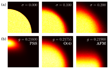
in place of $\Pi^{z}(\mathbf{q})$ in Eq. (3). For the AFM, we still use the $z$-component of the order parameter Eq. (3). In a state with both AFM and PSS order, the commutator $[m_{z},m_{p}]\propto L^{-2}$, and we can safely use the c-numbers corresponding to $m_{z}$ and $m_{p}$ from a given transition graph Sandvik_PRB_2010 to accumulate the joint probability distribution $P(m_{z},m_{p})$. For the putative O(4) symmetry to be manifest, we further normalize $m_{z}$ and $m_{p}$ by factors involving $\langle m_{z}^{2}\rangle$ and $\langle m_{p}^{2}\rangle$ sm .

For a point on an O(4) sphere of radius $R$, the projection onto two components results in a uniform distribution within a circle of radius $R$. However, in a finite quantum system we also expect fluctuations of $R$ and therefore compare our CBJQ results with a distribution obtained from an O(4) sphere with mean radius $R=1$ and standard deviation $\sigma$. Examples are shown Fig. 4. At the transition, the CBJQ distribution is rotation symmetric with radial profile similar to O(4) sampling with $\sigma\approx 0.15$. Inside the phases the distributions are shifted as expected—deep in the PSS we should eventually, for $L\to\infty$, obtain a point on the $y$-axis, and in the AFM state a line on the $x$-axis. Quantitative tests of the symmetry are presented in SM sm . As expected for an emergent symmetry, we find clear O(4) violations for small system sizes ($L=8,16$), but no detectable deviations at $g_{c}$ for the largest systems studied (up to $L=96$).

Having concluded that there is emergent O(4) symmetry, we can also understand why $1/\nu_{z,p}>3$ in Fig. 3(b): The dynamic exponent of the Anderson-Goldstone rotor states associated with O($N\geq 3$) order is $z=2$, and therefore one may expect the exponents to eventually tend to $d+z=4$ when $L\to\infty$ at $T=0$. The deviations may be due to $T>0$ effects when $T$ is scaled as $L^{-1}$ (instead of $L^{-2}$). As we show in SM sm , quantitative measures of the emergent O(4) symmetry in our $T=0$ calculations exhibit $L^{-4}$ scaling of the size of the $g$-window in which the symmetry is emergent.

Figure 4: (a) One quadrant of the sampled Muller_ACM_1959 distribution of two components of an O(4) vector with Gaussian length fluctuations with mean $R=1$ and standard deviation $\sigma$. (b) Projector QMC distribution $P(m_{z},m_{p})$ for the $L=96$ CBJQ model at three coupling ratios $g$. The $x$ axis represents the $z$ component of the AFM order parameter $m_{z}$, while the $y$-axis is the PSS order parameter $m_{p}$ sm .

Another interesting consequence of O(4) symmetry should be a specific logarithmic (log) form of the critical PSS temperature $T_{c}$ versus the distance $\delta=g_{c}-g$ from the $T=0$ transition point, $T_{\rm c}\propto\log^{-1}(C/\delta)$, as in an O($N\geq 3$) model with an Ising deformation Irkhin_PRB_1998 ; Cuccoli_PRB_2003 . This form is very different from that expected close to an Ising quantum-critical point, where $T_{\rm c}\propto\delta^{\nu_{\text{3D}}}$, where $\nu_{\text{3D}}$ is the 3D Ising correlation-length exponent. Neither form should apply at a conventional first-order transition extending from $(g_{c},T=0)$ to some $T>0$. If the O(4) breaking perturbation is very weak, one should still expect the log form to hold down to some low temperature.

Figure 5: Inverse PSS critical temperature versus the shifted coupling ratio $\delta=g_{c}-g$. The red line is a fit to the expected log form, and the black curve is of the conventional Ising form as a contrast. The inset shows examples of the extrapolation of $T_{c}$ using the expected critical scaling form with a subleading correction, $T_{c}=aL^{-b}(1+cL^{-d})$, with fitting parameters $a,b,c,d$ and $L$ up to $160$.

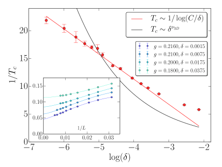
We have computed $T_{c}(g)$ for the PSS by the cumulant-crossing method using SSE data for $L\leq 160$. We can reliably extrapolate $T_{c}$ to the thermodynamic limit for $g\leq 0.216$ ($\delta\gtrsim 0.0015$), as shown in Fig. 5. The behavior for $\delta\lesssim 0.02$ is very well described by the log form, lending strong indirect support to the emergent O(4) symmetry through an important physical observable in the thermodynamic limit.

Discussion.—We cannot exclude that the O(4) symmetry is present only up to some length scale above the largest system, $L=96$, studied here. Such symmetry violations at a long scale may be expected at certain weak first-order transitions, either when the system is close to a fine-tuned point with order parameter of the higher symmetry (though no convincing emmergent symmetries were observed in connection with this scenario Kuklov04 ), or in proximity of a quantum-critical point at which the higher symmetry is emergent Nahum_PRL_2015 ; Wang_PRX_2017 ; Metlitski_2017 . In the latter case, perturbations break the symmetry above some length scale $\xi^{\prime}$ larger than the correlation length $\xi$ Wang_PRX_2017 .

In the CBJQ model studied here, the observed discontinuities are rather strong; from Fig. 3(c), the magnitude of the O(4) vector in AFM units is $m_{s}=\langle 4m_{z}^{2}\rangle^{1/2}\approx 0.12$, almost $25\%$ of the maximum staggered magnetization $1/2$. The first-order nature of the transition is apparent even on small lattices, e.g., as seen in the flow of $1/\nu_{z}$ toward an anomalously large value in Fig. 3(d). Thus, in the scenario of Ref. Wang_PRX_2017 , we should have $\xi\ll L\ll\xi^{\prime}\sim\xi^{1+a}$, where the exponent $a$ must be rather large in order to give the clear separation of length scales needed to account for the observed behavior. Such behavior has not been previously anticipated; rather, emergent symmetry on large length scales has been cited as support for continuous non-LGW transitions Nahum_PRL_2015 ; Sato_PRL_2017

In an alternative scenario of an asymptotic O(4) symmetry, the dominant symmetry-breaking field is tuned to zero at the AFM-PSS transition and higher-order O(4) violating perturbations would vanish upon renormalization, perhaps by an extension of the DQCP framework, or by some more general mechanism. While emergent O($N$) multicritical points arising from O($N-1$) and $Z_{2}$ order parameters have been extensively discussed within the LGW framework Hebert_PRB_2001 ; Pelissetto_2007 ; Hasenbusch_2011 ; Eichorn_2013 , the influence of the higher symmetry on associated first-order lines have not been addressed until recently in the weakly first-order DQCP context Wang_PRX_2017 . In order to exclude that the CBJQ model is accidentally fine-tuned to vanishing or extremely small perturbations of the O(4) symmetry, we have also studied a model extended by additional interactions; see SM sm .

We designed the CBJQ model with SrCu₂(BO₃)₂ in mind. The expected Ising-type $T>0$ PSS transition would be a good target for detecting the still incompletely characterized PSS phase and the putative O(4) symmetry. In 2D we have demonstrated a characteristic log form of $T_{c}$ (Fig. 5), and this form will hold down to some low temperature in the presence of sufficiently weak inter-layer couplings; presumably the 3D $T=0$ transition is a conventional first-order one.

The O(4) AFM–PSS transition is reminicent of the SO(5) theory of high-$T_{c}$ superconductivity demler04 , where O(3) AFM and O(2) superconducting order parameters form the higher symmetry; a scenario not confirmed, neither experimentally nor in models. After the completion of the present work, an SO(5) analogue of the AFM–PSS was demonstrated in a spin-$1$ $J$-$Q$ model Kaul18 , and an O(4) transition very similar to ours was discussed in the context of a classical 3D loop model Serna18 .

We present additional results supporting the existence of an emergent O(4) symmetry in the CBJQ model at its AFM–PSS transition. In Sec. 1, as a benchmark for finite-size scaling, we discusss results for the phase transition between an $xy$-ordered state and a $z$-ordered state in a deformed classical O(3) model (the XXZ model) below its critical temperature. In Sec. 2 we carry out a quantitative analysis of the order parameter histograms exemplified in Fig. 4 of the main paper. In Sec. 3 we deform the CBJQ model by introducing alternating plaquette terms of strength $Q_{A}$ and $Q_{B}$, such that the case $Q_{A}=Q,Q_{B}=0$ corresponds to the original CBJQ model discussed in the main text. We find emergent O(4) symmetry also with $Q_{B}=Q_{A}/2$, showing that the O(4) symmetry of the original CBJQ model is not accidental due to some implicit fine-tuning.

I.1 1. Classical XXZ model

In the 3D classical O($N$) model at $T<T_{c}$, a deformation of one of the $N$ interaction terms by a factor $\Delta$ leads to an ordered phase breaking O($N-1$) symmetry for $\Delta<1$ and $Z_{2}$ (Ising) symmetry for $\Delta>1$. We have argued that the CBJQ model corresponds to this situation with $N=4$, with the $O(3)$ and $Z_{2}$ phases corresponding to the AFM and PSS, respectively. However, in the CBJQ model the O(4) symmetry is not explicitly present at the Hamiltonian level but is emergent on long length scales.

We will here study the deformed 3D classical O(3) model and demonstrate finite-size scaling behaviors analogous to those that we found for the CBJQ model. We could also have studied an O(4) model, but the same physics is manifest already with $N=3$, which is the minimum number of components for which one of the deformed phases breaks a continuous symmetry and the other one breaks the discrete $Z_{2}$ symmetry. The Hamiltonian of the XXZ model is:

$$H=-\sum_{\langle ij\rangle}\sigma^{x}_{i}\sigma^{x}_{j}+\sigma^{y}_{i}\sigma^{y}_{j}+\Delta\sigma^{z}_{i}\sigma^{z}_{j},$$ (S1)

where $\langle ij\rangle$ corresponds to nearest-neighbor interactions between the unit vectors $\mathbf{\sigma}_{i}$ on a simple cubic lattice. We could also consider the 2D $S=1/2$ AFM Heisenberg model at $T=0$ with a similar deformation, which was done in Ref. Cuccoli_PRB_2003, but with a different focus.

The 2D $S=1/2$ XXZ model with nearest-neighbor interactions on the square lattice has long-range order at $T=0$ for all values of $\Delta$, and the order parameter symmetry changes with $\Delta$ in the same way as in the 3D classical model below $T_{c}$. When passing through the special point $\Delta=1$, the elementary excitations change, as the Goldstone modes present in the O(2) phase and the O(3) point are gapped out continuously for $\Delta>1$. In this sense, we can consider the change in symmetry as a phase transition with both first-order and continuous characteristics; a discontinuous flip of the direction of the order parameter but a continuously varying gap. Note that $T>0$ in the quantum XXZ model corresponds to a finite size $L_{3}\propto 1/T$ of one of the dimensions of the classical 3D model (here written as the third dimension). Here we will only conside the 3D model with equal size $L$ in all dimensions and, thus, obtain results corresponding to $T=0$ in the quantum case when $L\to\infty$.

We have carried out Monte Carlo simulations of the classical 3D XXZ model at two different temperatures in the ordered phase, $T^{-1}=0.7$ and $0.75$, the former being close to $T^{-1}_{c}(\Delta_{c}=1)\approx 0.6930$. We use the efficient Wolff cluster agorithm wolff_alg and analyze the $xy$ and $z$ magnetizations individually. The Binder cumulants and slopes are defined in ways analogous to Eqs. (5) and (6).

As shown in Fig. S1, behaviors very similar to those in the CBJQ model (Fig. 3) are observed at At $T=0.7$ if we make an analogy between the $xy$ magnetization and the AFM order parameter on the one hand and the Ising $z$ magnetization and the PSS order parameter on the other hand. There are no negative cumulant peaks in Fig. S1(a) in the neighborhood of the transition point $\Delta=1$. In Fig. S1(b) we show that the transition point is accurately reproduced with the same curve-crossing method as we used for the CBJQ model. Looking at the coexistence values of the order parameters in Fig. S1(c), which obey $\langle m^{2}_{x}\rangle+\langle m^{2}_{y}\rangle=2\langle m^{2}_{z}\rangle$, the length $|m|$ of the vector ${\bf m}$ is about 25% of the maximum value $1$. This is similar to the relative length of the O(4) vector extracted from Fig. 3(c) for the CBJQ model, where we can define $|m|=\sqrt{4\langle m_{z}^{2}\rangle}$, with maximum value $|m|=1/2$.

In Fig. S1(d) we see that $1/\nu_{xy}$ extrapolates close to the standard first-order value $3$, while $1/\nu_{z}$ is somewhat lower. One may question the standard first-order value in this case because of the lack of free-energy barriers, but a simple mean-field argument gives that the relevant scaling variable is $(\Delta-1)L^{3}$ also for the long-range ordered XXZ model. In Fig. S1(d) we have only used a simple line fit to extrapolate both the exponents, and an asymptotically form with higher-order corrections and larger system sizes would likely explain why the values are less than $3$. Similar to the CBJQ model, Fig. 3(d), there is a rather sharp cross-over from one slope at small system sizes to a higher slope for the larger sizes. The cross-over region should correspond to $L\approx\xi$, $\xi$ being the correlation length of the infinite system in the neighborhood of the transition. Because of the cross-over behavior, it is difficult to carry out reliable extrapolations with the rather small number of system sizes available.

In most respects, we see that the O(3) order–order transition looks in finite-size scaling like a first-order transition, with the glaring exception of the lack of negative Binder peak. Indeed, with phase coexistence in the form of a higher symmetry, the arguments behind the negative peak Vollmayr_ZPB_1993 ; Iino_ArX_2017 do not apply, since, thanks to the higher rotational symmetry, the two phases are not separated by a free-energy barrier at the transition point $\Delta=1$. These results for the classical model provide support for a similar mechanism at play at the AFM–PSS transition of the CBJQ model, even though no exact higher symmetry is present in its Hamiltonian.

In Fig. S2 we show results at a slightly lower temperature, $T^{-1}=0.75$. The results are qualitatively very similar to those at $T^{-1}=0.7$, but the features are sharper due to the stronger order. The extrapolation of both exponents $1/\nu_{xy}$ and $1/\nu_{z}$ to $3$ is also clearer in this case, with an overall weaker size dependence (though still the linear extrapolation somewhat underestimates the values of both the exponents) and no clear cross-over. The lack of cross-over here suggests that the correlation length in the infinite system remains small at this temperature.

Figure S1: Results for the classical 3D Heisenberg with anisotropy $\Delta$ at $T^{-1}=0.7$, graphed as in Fig. 3 in the main paper; the $xy$ and $z$ Binder cumulants vs $\Delta$ in (a), the crossing points extrapolated in $1/L$ to the phase transition point in (b), the coexistence values of the squared order parameters versus $1/L$ in (c), and the correlation-length exponents extrated from the slopes of the cumulants in (d). The system sizes in (a) are $L=8$ (black),$16$ (blue) and $32$ (red), with open and solid symbols used for $U_{xy}$ and $U_{z}$, respectively.

Figure S2: The same quantities as in Fig. S1 for the 3D XXZ model at a lower temperature, $T^{-1}=0.75$.

I.2 2. Quantitative check of emergent O(4) symmetry

Here we discuss further details of our tests of emergent O(4) symmetry in the CBJQ model based on order-parameter distributions (histograms) $P(m_{z},m_{p})$ such as those shown in Fig. 4. In addition, we also consider the distribution of $P(m_{s},m_{p})$, where $m_{s}$ is the magnitude of the full $O(3)$ AFM order parameter,

$$m^{2}_{s}=m_{x}^{2}+m_{y}^{2}+m_{z}^{2}.$$ (S2)

Like $m_{p}$ defined in Eqs. (3) and (7), the c-number corresponding to $m_{s}^{2}$ is obtained in the valence-bond projector QMC method after each Monte Carlo updating sweep directly from the transition graph as a single unique number (in contrast to just the component $m_{z}$, which is obtained by sampling one of the many spin configurations that contribute to the transition graph) Sandvik_PRB_2010 ; Liang1988 ; Beach2006 . Note that it is not possible to obtain independent equal-time values for all three components of the AFM order parameter from the transition graphs or the associated $z$ basis spin configurations.

In the simulations, we generate and store a list of points $(m_{z},m^{2}_{s},m_{p})_{i}$, $i=1,\ldots,M$. In order to obtain smooth probability distributions and small error bars on the associated integrated quantities that we use to test for the emergent symmetry, we need a very large number of points ($M$ of the order of millions). To capture the point of maximal symmetry and study the scaling properties away from this point, we also need many values of $g$. We have carried out the valence-bond QMC simulations with a very long projection time $\tau$ in the imaginary-time evolution operator ${\rm e}^{-\tau H}$ and find that $\tau=8L$ is sufficient for $T\to 0$ convergence of the distributions for the system sizes consiedered here; up to $L=96$.

Symmetry tests with two components.—The definitions of the two order parameters by Eqs. (3) and (7) are not unique. Therefore, even if there is an emergent symmetry between the order parameters, $m_{z}$ and $m_{p}$ are not directly comparable as to their overall magnitudes. To investigate a possible emergent O(2) symmetry of the distribution $P(m_{z},m_{p})$, as a proxy for the full O(4) symmetry of all four components, we need to remove the ambiguity by properly normalizing the sampled numbers. To this end, post-simulation, we compute the corresponding variances $\langle m_{z}^{2}\rangle$ and $\langle m_{p}^{2}\rangle$. We can then define the radius $R$ of the distribution as

$$\langle R^{2}\rangle=\langle m_{z}^{2}\rangle+a^{2}\langle m_{p}^{2}\rangle,\leavevmode\nobreak\ \leavevmode\nobreak\ \leavevmode\nobreak\ \leavevmode\nobreak\ R\equiv\langle R^{2}\rangle^{1/2},$$ (S3)

while also requiring that

$$\langle m_{z}^{2}\rangle=a^{2}\langle m_{p}^{2}\rangle.$$ (S4)

Thus, the parameter $a$ that puts the two sampled order parameters on an equal scale is defined by

$$a^{2}=\frac{\langle m_{z}^{2}\rangle}{\langle m_{p}^{2}\rangle}.$$ (S5)

We can now define normalized point pairs as

$$(\tilde{m}_{z},\tilde{m}_{p})=R^{-1}(m_{z},am_{p}),$$ (S6)

and test for emergent O(2) symmetry in the distribution $P(\tilde{m}_{z},\tilde{m}_{p})$ at the AFM–PSS transition.

To quantify the degree of O(2) symmetry of a distribution $P(\tilde{m}_{z},\tilde{m}_{p})$ we use the integrals

$$I_{q} = \int\text{d}\tilde{m}_{z}\text{d}\tilde{m}_{p}P(\tilde{m}_{z},\tilde{m}_{p})\cos\bigl{(}q\phi(\tilde{m}_{z},\tilde{m}_{p})\bigr{)}$$ (S7)

$$= \frac{1}{M}\sum_{i=1}^{M}\cos(q\phi(|\tilde{m}_{z}|,|\tilde{m}_{p}|)_{i}),$$

where on the second line $i$ is the index corresponding to the $M$ QMC sampled points $({m}_{z},{m}_{p})_{i}$, from which angles $\phi(|\tilde{m}_{z}|,|\tilde{m}_{p}|)_{i}\in[0,\pi/2]$ are extracted (with the absolute values taken to transform to the positive quadrant). We will here consider the integrals with $q=2,4,6,8$, all of which should vanish if the distribution is O(2) symmetric. For larger $q$, the results become increasingly noisy, but since there is no reason to expect distributions with $I_{2}=I_{4}=I_{6}=I_{8}=0$ and $I_{q>8}\not=0$, what we do here is sufficient for demonstrating O(4) symmetry.

There is a remaining ambiguity in the normalization, as to the point at which the scale factor $a$ should be evaluated. In Fig. 4(b) of the main paper, $a$ was evaluated at $g=0.21755$ (the data in the middle panel) and used at the other $g$ values as well. If the distribution is O(2) symmetric at $g_{c}$, as it appears to be, we argue that the best way to proceed is to fix $a$ at this point, instead of using a $g$-dependent value $a^{2}(g)$ computed from a distribution that is not O(2) symmetric when $g\not=g_{c}$. This choise is motivated by the fact that the O(4) symmetry should only apply to a single point, the transition point, and there is no reason why the normalization condition Eq. (S4) should be applied elsewhere. If the varying $a^{2}(g)$ is used for all values of $g$, then the distribution away from $g_{c}$ will artificially be drawn out in one directon, thus making the signals (the values of $I_{q}$) less sensitive to the control parameter. The fact that the mean vector projection in the different directions should not be the same when the vector flips from the AFM sector to the PSS direction would then be missed. Note that fixing $a^{2}(L)$ at $g_{c}$ also in no way can artificially introduce a false symmetry in the quantities we study.

Figure S3: The dependence on the coupling $g$ and system size $L$ of the order-parameter normalization ratio $a^{2}$ defined in Eq. (S5).

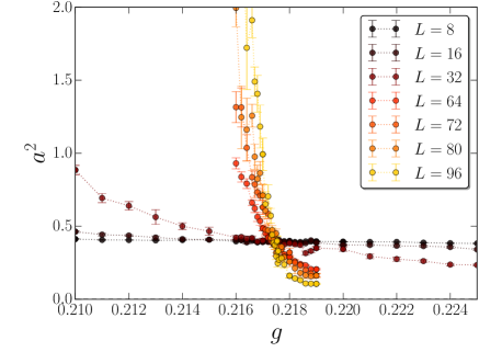
Given the above arguments, we use the following two-step procedure to analyze the distribution: At the first stage, we compute the scale factor $a^{2}(g)$ in Eq. (S5) for each of the $g$ values considered. Results for various system sizes up to $L=96$ are shown in Fig. S3. We can observe that the curves for different system sizes cross each other around the transition point $g\approx 0.2175$. Based on closer inspection and extrapolations of the crossing points, in the calculations of $I_{q}$ for for all $g$ and $L$ we fix $a(L)$ in Eq. (S4) at their values obtained at $g=0.21755$, which is full consistent with the transition point $g_{c}=0.2175\pm 0.0001$ extracted in the main paper.

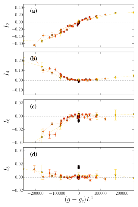
The results are shown in Fig. S4. Here we can see that the $I_{q}$ curves for odd $q$ go through zero at $g_{c}$, while for even $q$ they exhibit minimums at $g_{c}$. For the larger system sizes, $I_{4}$ and $I_{8}$ have minimum values equal to $0$ to within statistical errors. Thus, we conclude that there is an emergent O(4) symmetry at the transition point. Deviations from O(4) behvior are seen in $q_{4}$ and $I_{8}$ for the smallest system sizes, which is expected if the symmetry is emergent upon increasing $L$. For the largest system sizes, up to $L=96$, no deviations from O(4) symmetry can be detected at $g_{c}$ in any of the $I_{q}$ integrals.

Figure S4: Tests of emergent O(4) symmetry, using the integrals $I_{2}$ (a), $I_{4}$ (b), $I_{6}$ (c), and $I_{8}$ (d). The value of the re-scaling parameter $a(L)$ in Eq. (S5) is held fixed at the value obtained in Fig. S3(c) at the point $g=0.21755$. The symbol colors correspond to the system sizes as in Fig. S3.

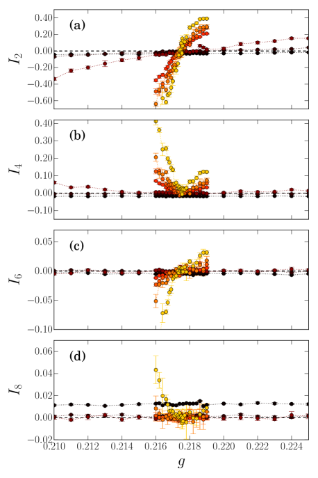
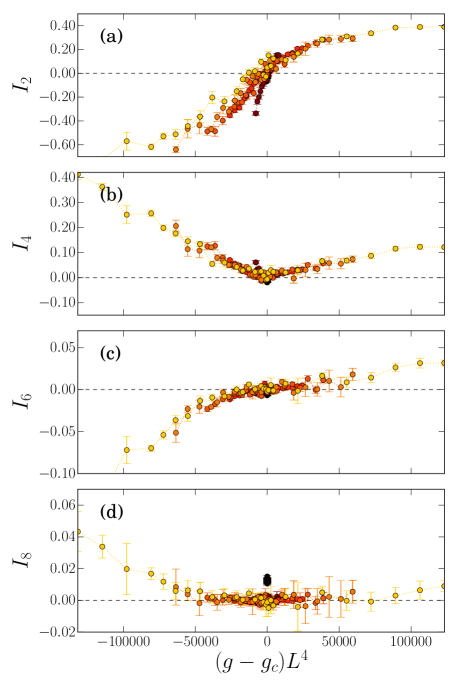
We next carry out a data-collapse procedure with the data in Fig. S4. At a classical first-order phase transition, the exponent $\nu$ relevant for finite-size scaling slightly away from the phase transition takes the trivial value $\nu=1/d$ Vollmayr_ZPB_1993 ; Iino_ArX_2017 . In analogy with the case of quantum-critical points, one would expect that $d$ at a quantum first-order phase transition should be replaced by $d+z$, $z$ being the dynamic exponent that relates time and length scales. In the case at hand, one would expect $z=2$, which corresponds to the scaling of the finite-size excitation gap, $\epsilon\propto L^{-2}$, in a 2D O(N) system. The time scale $\epsilon^{-1}$ corresponding to this energy is exactly that of the angular fluctuations of the order parameter, as in Anderson’s analogy between the finite-size excitations of an AFM and quantum rotor states (as studied explicitly in QMC calculations in Ref. Phil17 ). Thus, we expect $1/\nu=z+2=4$ to be the relevant scaling exponent describing the rotation of the O(4) vector as the transition point is traversed, and we attempt to describe the data by the finite-size scaling form

$$I_{q}(g,L)=f_{q}[(g-g_{c})L^{4}].$$ (S8)

In Fig. S5 we re-graph the data from Fig. S4 versus $(g-g_{c})L^{4}$. We indeed observe very good collapse of the data, except for the smallest systems. These results lend additional support to an emergent O(4) symmetry.

It should be noted here that we did not see clearly that $1/\nu_{xy}$ and $1/\nu_{z}$ extrapolate to $4$ in Fig. 3(d). There could be two reasons for this. First, as we mentiond also in Sec. 1 above, we have neglected corrections to the assumed leading linear scaling forms in Fig. 3(d). Second, since the excitation gap at the transition should scale as $1/L^{2}$, there may be some effects of using $1/T\propto L$, instead of $1/T\propto L^{2}$, in the SSE simulations. This would not affect any of the other extrapolated quantities in Fig. 3, as it is still true that $T\to 0$ when $L\to\infty$ and the O(4) coexistence state should have an exponentially large correlation length $\xi(T)$ as $T\to 0$. i.e., $\xi(T)\gg L$ when $T\propto 1/L$. The projector QMC simulations used here to generate the order-parameter simulations are also fully consistent with coexisting long-range orders and the value of the transition point extracted based on SSE simulations. As we have seen above, the quantitative scaling analysis of the symmetry properties gives further support to the emergent O(4) symmetry in the complete absence of any finite-$T$ effects.

Figure S5: Tests of data collapse of $I_{q}(g,L)$ based on Eq. (S8). The data points are the same as in Fig. S4, but the coupling has been rescaled by a factor $L^{4}$ relative to the critical point, for which we here use $g_{c}=0.21755$, which is within the statistical errors of the value determined in the main paper.

Along with a finite order parameter at the transition, the O(4) symmetry projected down to two components also implies a flat radial distribution between $0$ and the radius $R$ of the sphere. As we pointed out in the main text and demonstrated in Fig. 4, the not completely flat behavior close to the rim observed in the CBJQ histogram can be explained by finite-size fluctuations of the radius, which should vanish only in the limit $L\to\infty$. Furthermore, since the O(3) symmetry between the three components of the AFM order parameter is explicitly enforced by the Hamiltonian and is also not violated in any way in the simulations, the demonstration of O(2) symmetry in the distribution $P(m_{z},m_{p})$ immediately also implies O(4) symmetry at the AFM-PSS coexistence point.

Thus, we have shown here that for the largest system size available, $L=96$, the CBJQ model has a point at which its combined AFM and PSS order parameters exhibit O(4) symmetry to a high degree, with any potential violation too small to be detectable within the rather small error bars of our results. For the smallest system sizes we do see some deviations from perfect symmetry, which is expected when the symmetry is not present in the hamiltonian but emerges as the system size increases.

Figure S6: Test of emergent O(4) symmetry of the CBJQ involving all four order parameter components. The $x$ axis represents the magnitude of the total AFM order parameter $m_{s}$, defined in Eq. (S2), and the vertical axis the PSS order parameter $m_{p}$. Only the quadrant with all positive values is shown. Panels (a) are for the case of a perfect O(4) sphere with radius $R=1$ and variance $\sigma^{2}$, sampled using the algorithm in Ref. Muller_ACM_1959 . Panels (b) show valence-bond projector QMC results for the CBJQ model at three values of $g$; inside the PSS phase, close to the transition point with emergent O(4) symmetry, and inside the AFM phase.

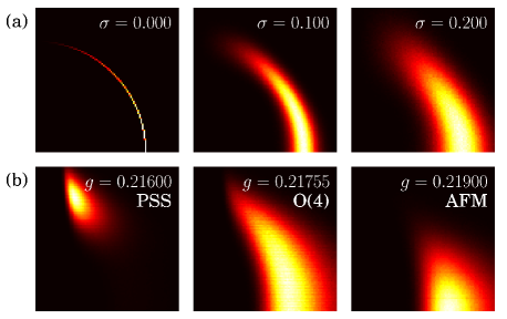
Tests with four components.—We complement the above analysis of two out of the four components of the putative O(4) vector with a test where all four components are used, projected down to two dimensions by using the magnitude of the full O(3) AFM order parameter in Eq. (S2) and the PSS order parameter, i.e., the distribution $P(m_{s},m_{p})$. We carry out a process similar to the one discussed above to put the overall lengths of the AFM and PSS components on equal footing.

For an ideal O(4) sphere with fixed $R$ projected down to two dimensions in this manner, the distribution $P(m_{s},m_{p})$ has the shape of arc of infinitesimal thickness and radius $R$, with the density varying proportionally to $m_{s}^{2}$ along the arc, due to the different contents (number of components of the 4-dimensional vector) of the two dimensions. Fig. S6(a) shows the distribution for three different values of the standard deviation $\sigma$ of the fluctuating radius about the mean value $R=1$. In the case of the CBJQ model, as shown in Fig. S6(b), there is indeed very little weight close to the y-axis as expected. As we go from the PSS state to the AFM state the weight shifts clockwise from large $y$ ($m_{p}$) values down toward the $x$-axis (large $m_{s}$). At the transition point we see a distribution very similar to the O(4) sphere with $\sigma\approx 0.20$

It should be noted that $m_{s}^{2}$ in the valence-bond basis is obtained from the transition graph as a sum of squared loop lengths, and this corresponds to a sum over $2^{n_{l}}$ spin configurations in the basis of $S^{z}$ spins, $n_{l}$ being the number of loops (each loop having two compatible staggered spin configurations). This implicit averaging over points on the putative O(4) sphere may cause some additional smearing in $P(m_{s},m_{p})$, beyond just the projection down to two dimensions and the fluctuations of the radius associated with finite system size. The somewhat larger $\sigma$ required to match the O(4) sphere in Fig. S6 than what was needed in the case of $P(m_{z},m_{p})$ in Fig. 4 likely reflects this effect. In addition, for finite system size, the loop estimator for $m_{s}$ has a strict lower bound $\propto L^{-2}$, with a de facto large prefactor, and this also seems to cause some visible deviations from the O(4) sphere results at the left tip of the distribution. For these reasons, we believe that the $P(m_{z},m_{p})$ distribution is better for quantitatively characterizing the degree of symmetry.

I.3 3. The CBJQ model with $Q_{A}\not=Q_{B}$

Figure S7: Data collapse of the integrals $I_{q}(g,L)$ for the extended CBJQ model with $Q_{B}=Q_{A}/2$, based on Eq. (S8). The system sizes are up to $L=96$, with the symbols color-coded as in Fig. S3.

One might wonder whether the CBJQ model could have an accidental emergent symmetry, i.e., that a generically present symmetry-breaking perturbation at the transition point could be absent, or extremely small, in this particular model. In order to exclude such a fine-tuning scenario, we here deform the CBJQ model in a significant way by introducing four-spin coupling of strenth $Q_{B}$ on the plaquettes without $Q$-couplings in Eq. (1) and Fig. 1. We refer to the previously present plaquette couplings as $Q_{A}$. Calling the two sets of plaquettes $\Box_{A}$ and $\Box_{B}$, the Hamiltonian of this extended CBJQ model is

$$H=-J\sum_{\langle ij\rangle} P_{ij}-Q_{A}\hskip-5.69054pt\sum_{ijkl\in\Box_{A}}\hskip-2.84526pt(P_{ij}P_{kl}+P_{ik}P_{jl})$$ (S9)

$$-Q_{B}\hskip-5.69054pt\sum_{ijkl\in\Box_{B}}\hskip-2.84526pt(P_{ij}P_{kl}+P_{ik}P_{jl}).$$

When $Q_{A}=Q_{B}$, this model becomes the ordinary $J$-$Q$ model on the square lattice, which hosts a four-fold degenerate columnar VBS and where no convincing signs of a first-order transition between it and the AFM has been detected. The non-magnetic state in the extended CBJQ model is likely a two-fold degenerate PSS for any $Q_{A}\not=Q_{B}$, though this is not completely clear because the checkerboard deformation of the square-lattice system is still also compatible with a four-fold degenerate columnar VBS. If indeed we have the PSS for all $Q_{A}\not=Q_{B}$, then for $Q_{A}$ very close to $Q_{B}$ there will be interesting cross-over behaviors as the system size is increased, from an almost $Z_{4}$ symmetric columnar VBS to a $Z_{2}$ symmetric PSS. However, the first-order behavior we have found here for $Q_{B}=0$ may in principle end at a tricritical point at some $0<(Q_{B}/Q_{A})_{t}<1$, with a continuous AFM–PSS transition obtaining for $(Q_{B}/Q_{A})_{t}<Q_{B}/Q_{A}<1$. In a future study, we plan to investigate these and other issues for the extended CBJQ model in its full range of the ratio $Q_{B}/Q_{A}$.

Here we only consider $Q_{B}/Q_{A}=1/2$, for which we find that the transition is still first-order and the nonmagnetic state is indeed the PSS. We focus on the histogram approach for detecting emergent O(4) symmetry. The added interaction is sufficiently strong so that an accidental emergent symmetry cannot be the explanation for our finding for $Q_{B}/Q_{A}=0$ if we also find O(4) symmetry when $Q_{B}/Q_{A}=1/2$—unless this whole class of extended CMJQ models is automatically fine-tuned, which by itself would be remarkable and an indication that symmetry perturbations can be broadly avoided (likely beyond the CBJQ models) under previously overlooked circumstances.

We proceed using the same methods as previously, here up to system size $L=96$. We find $g_{c}=0.139\pm 0.001$ and the length of the O(4) vector with the same normalization as in the previous section is about 10% of the maximum value, or $40\%$ of the value found when $Q_{B}=0$. Scaled results for the integrals $I_{q}$ are shown in Fig. S7. Here we observe the same kind of behavior as in Fig. S5, with good data collapse and no discernible deviations from $0$ of the $I_{q}$ values at $g_{c}$. Thus, we conclude that the emergent O(4) symmetry is not due to some accidental fine-tuning but an intrinsic feature of the CBJQ class of models.

Comparing Figs. S5 and S7, we see that the scaled integrals are close to zero over a wider range of $(g-g_{c})L^{4}$ when the first-order transition is weker, i.e., for $Q_{B}/Q_{A}=1/2$. This is natural in light of the larger fluctuations as the discontinuities of the order parameters weaken. The behavior also points to an important role of a quantum-critical point that may be reachable as $Q_{B}/Q_{A}$ is further increased (but not up to $Q_{B}/Q_{A}=1$, where the non-magnetic state is different, a columnar VBS breaking $Z_{4}$ symmetry). The emergent symmetry may ultimately be connected to some extension of the DQCP scenario, as also mentioned in the main paper.

These results of course do not prove that the emergent symmetry exists up to infinite length scale. In the scenario of an approximate symmetry at the first-order transition being due to a nearby critical point with exact emergent symmetry, one would expect the length scale up to which the apprpximate symmetry applies to be larger when the order parameter is smaller. Therefore, it would clearly be useful to also study a model where the coexisting order parameters are larger than for the case $Q_{B}=0$. However, so far we have not found any way to make the transition more strongly first-order within the CBJQ models.