The Photometric Selection of M-dwarfs using Gaia, WISE and 2MASS photometry

Abstract

We present criteria for the photometric selection of M-dwarfs using all-sky photometry, with a view to identifying M-dwarf candidates for inclusion in the input catalogues of upcoming all-sky surveys, including TESS and FunnelWeb. The criteria are based on Gaia, WISE and 2MASS all-sky photometry, and deliberately do not rely on astrometric information. In the lead-up to the availability of truly distance-limited samples following the release of Gaia DR2, this approach has the significant benefit of delivering a sample unbiased with regard to space velocity. Our criteria were developed by using Galaxia synthetic galaxy model predictions to evaluate both M-dwarf completeness and false-positive detections (i.e. non-M-dwarf contamination rates). We have derived two sets of Gaia G < 14.5 criteria – a “high-completeness” set that contains 78,340 stars, of which 30.7-44.4% are expected to be M-dwarfs and contains 99.3% of the total number of expected M-dwarfs; and a “low-contamination” set that prioritises the stars most likely to be M-dwarfs at a cost of a reduction in completeness. This subset contains 40,505 stars and is expected to be comprised of 58.7-64.1% M-dwarfs, with a completeness of 98%. Comparison of the high-completeness set with the TESS Input Catalogue has identified 234 stars not currently in that catalogue, which preliminary analysis suggests could be useful M-dwarf targets for TESS. We also compared the criteria to selection via absolute magnitude and a combination of both methods. We found that colour selection in combination with an absolute magnitude limit provides the most effective way of selecting M-dwarfs en masse.

1 Introduction

M-dwarfs comprise around 75% of the stars in our Milky Way (Tarter et al., 2007), making them the most common type of star in our Galaxy. Up to 50% of these stars may harbour terrestrial exoplanets (Kopparapu, 2013). The low masses and luminosities of M-dwarfs also mean that their habitable zones correspond to relatively short-period orbits (< 100 d), making them prime targets for upcoming exoplanet transit surveys, (e.g. NASA’s Transiting Exoplanet Survey Satellite (TESS); Ricker & MORE, 2009), and ground-based Doppler follow-up to measure planetary masses and densities.

TESS will download full-field images sampled every 30 minutes (Ricker & MORE, 2009), allowing it to detect potentially habitable M-dwarf exoplanets over the whole sky down to around 14th magnitude. In addition, it will download data for a constrained number of target stars ($\sim$ 200,000) in its high cadence mode (sampling every 2 minutes). Clearly, it is desirable to know as much as possible about the best, high priority M-dwarf candidates in advance of TESS starting its survey. In the absence of spectroscopic data for every star in the sky down to TESS’s faint magnitude limit, the next best strategy is selecting likely M-dwarfs using either astrometric or photometric information.

The use of astrometric selection has dominated M-dwarf identification to date (e.g. Luyten 1979; Zacharias et al. 2000), with proper motion (and especially the reduced proper motion H; Luyten 1922) being used to identify stars likely to be close to the Sun (and therefore low in luminosity). This does have the disadvantage, however, of only probing two components of each star’s three-dimensional space motion, and so necessarily produces a biased sample.

Photometric M-dwarf selection suffers from contamination by non-M-dwarfs due to photometric uncertainties, source contamination and the intrinsic scatter of stellar properties about any adopted relationships between observed colours and physical parameters. On the other hand, they do not suffer any kinematic bias, and there are now very large, high-quality and publicly available all-sky databases at the optical and near-infrared wavelengths best suited to M-dwarf selection. This paper, therefore, explores the photometric approach.

The standard practice for fully and completely identifying M-dwarfs is through initial candidate selection using either photometry or astrometry (or both), followed by spectral classification. To date, obtaining spectroscopy for every possible M-dwarf in the sky down to the relevant magnitudes for TESS (i.e. Gaia G$\approx$14.5, I$\approx$14) has been infeasible. No instrument has had the combination of a sufficiently wide-field (5-10$\degree$ diameter field-of-view), aperture in the $>$1 m range, and multi-object spectroscopic capability for hundreds of objects across that wide-field.

This is now changing. Both the FunnelWeb survey in the southern hemisphere, and LAMOST (Chu & Cui, 1996) in the northern hemisphere, can observe hundreds of targets (or more) over fields of 30 square degrees or more, with reconfiguration times between fields measured in minutes. These dedicated survey facilities now make it possible to observe tens of thousands of stars per night (or millions of stars per year), making possible a new generation of magnitude-limited, all-sky survey.

FunnelWeb (Rains et al. 2018, in prep.) is is a multi-object stellar survey of the Southern Hemisphere set to commence observations in July 2018. It will cover the entire southern sky (excluding only the most crowded regions with $\delta\leq 0\degree$, $|b|\geq 10\degree$) and obtain high-quality (S/N 100) optical spectra for some $\sim$ 1.8 million stars down to a magnitude of Gaia G=14.5, aiming for 99% completeness at the G=12.5 level. The survey is enabled by the TAIPAN instrument on the recently refurbished 1.2 m UK-Schmidt Telescope at Siding Spring Observatory, which is able to simultaneously robotically position 150 optical fibres (or “Starbugs”) within a 6°field of view. The instrument operates over the wavelength range 3700-8700Å, and has a spectral resolution of R $\geq$ 2000. The main goals of the survey include a spectral library with detailed stellar parameters (including T_eff, log(g), [Fe/H] and [$\alpha$/Fe]), including stellar spectra for targets being observed by the TESS satellite, with M-dwarfs a particular focus.

The combination of these new facilities, and the availability of large, deep and all-sky multi-colour surveys like Gaia (Gaia Collaboration et al., 2016a), the Two Micron All-Sky Survey (2MASS; Skrutskie et al. 2006), the Wide-field Infrared Survey Explorer data (WISE; Wright et al. 2010) and the Skymapper survey (Keller et al., 2007) makes it eminently plausible to use of photometric M-dwarf selection, followed by the spectroscopic confirmation, for extremely large numbers of candidate M-dwarfs. However, even with the ability to observe a million stars per year, it is clearly still desirable to refine the criteria for selection of M-dwarf candidates as much as possible – and in particular to understand the completeness and contamination that can be expected from a given set of photometric selection criteria. This is the focus of this paper.

2 Data

2.1 Survey Data

The Gaia, WISE and 2MASS all-sky surveys provide photometry at a range of optical and near-infrared wavelengths. In particular, as can be seen from Figure 1, they probe critical wavelengths for the selection of M-dwarfs, which emit most of their flux between 0.6 nm and 5 $\mu$m).

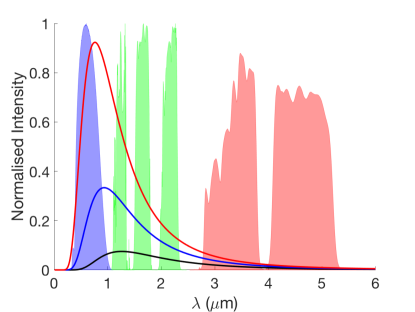
Figure 1: The wavelength coverage of the Gaia G (blue), 2MASS J, H and K bands (green) and the WISE W1 and W2 bands (red) with black body curves at temperatures 3800, 3100 and 2300K that are each representative of a M0, M4 and M9 M-dwarf continuum (red, blue and black lines respectively).

We selected a working dataset of all objects from Gaia DR1 (Gaia Collaboration et al., 2016b) with G $<$ 14.5 and cross-matched against the 2MASS PSC and WISE AllWISE catalogues using the Gaia DR1 portal ADQL. We limited the area of sky selected to that accessible from the southern hemisphere ($\delta$ < +10 °) and avoided the Galactic plane ($|$b$|>$10 °) – the latter criterion was adopted because the large WISE full-width-at-half-maximum of $\approx$ 6 " makes it difficult to match, or rely on, its data in crowded fields. Any object flagged in the AllWISE catalogue as a galaxy (xscproc $\neq$ null), an extended object (ext_flg $\neq$ 0), as multiple objects (n_2mass > 1) or as objects with poor/contaminated photometry (cc_flags $\neq$ 0000) was also removed. The resulting catalogue contains almost 9 million stars, with 6.2 million stars at G < 14.5, and Figure 3a shows the number density of resulting sources in an example J–W1/W1–W2 colour-colour plane.

2.2 Spectroscopic Comparison Sample

To provide a comparison set of photometry for stars with known spectral classifications, we extracted the same Gaia, 2MASS and WISE photometry for the large sample of M-dwarfs spectrally classified by West et al. (2011), supplemented by the late K-dwarfs classified by Zhong et al. (2015). To ensure the most precise photometry was used for these known M- and K-dwarfs, we only included stars in this comparison sample if they were quiescent for the bands we used using (var_flg = XX__, where X is from 0-5). Otherwise this comparison sample was selected in the same manner as our main sample.

We calculated median colours and the r.m.s. scatter about the mean for each spectral type and these are plotted for J–W1/W1–W2 in Figure 4, along with linear parametrisations of the median colours. The results of these parametrisations are tabulated in Table 1 as a function of spectral type and seen in Figure 2. In general the photometric scatter around these linear relationships are large – usually several tenths of a magnitude – with the scatter for optical-infrared colours becoming as large as seven-tenths of a magnitude at early types. This is much larger than expected due to the photometric measurement uncertainty of these surveys, suggesting this scatter is dominated by cosmic scatter due to metallicity variations, age variations, unresolved binarity, etc. Nonetheless, the trends with spectral type are consistent and smoothly varying.

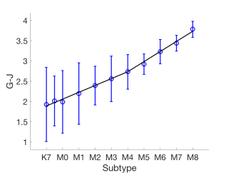
(a)

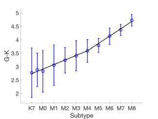
(b)

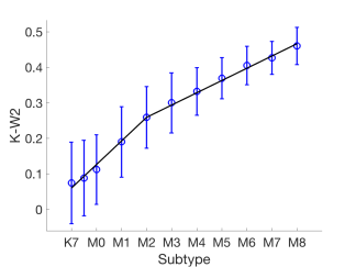
(c)

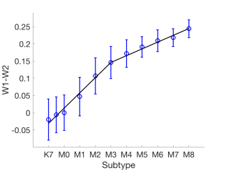
(d)

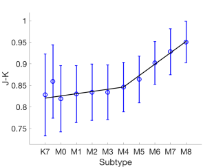
(e)

Figure 2: Photometric Gaia/2MASS/WISE colours as a function of spectral type for M-dwarfs of West et al. (2011) and late K-dwarfs of Zhong et al. (2015). Circles are the median colour values for each subtype, with uncertainty bars showing r.m.s scatter. The solid black lines are linear fits to the median subtypes. The outlier K7.5 median colour value for J–K was excluded when determining that parameteristion.

Type	N	G–J	r.m.s.	G–K	r.m.s.	K–W2	r.m.s.	W1–W2	r.m.s.	Src
K7	421	1.89	0.808	2.737	0.81	0.06	0.11	-0.031	0.059	ZJ
K7.5	311	1.974	0.771	2.822	0.773	0.093	0.107	-0.009	0.057	ZJ
M0	1268	2.058	0.733	2.907	0.736	0.126	0.103	0.013	0.055	WA
M1	1121	2.227	0.658	3.077	0.662	0.193	0.095	0.057	0.051	WA
M2	1493	2.396	0.583	3.246	0.588	0.259	0.088	0.102	0.047	WA
M3	2012	2.564	0.508	3.416	0.514	0.294	0.08	0.146	0.043	WA
M4	1974	2.733	0.433	3.585	0.44	0.328	0.072	0.166	0.04	WA
M5	732	2.983	0.358	3.859	0.366	0.363	0.065	0.185	0.036	WA
M6	311	3.232	0.283	4.132	0.292	0.397	0.057	0.205	0.032	WA
M7	128	3.482	0.208	4.406	0.218	0.432	0.049	0.225	0.028	WA
M8	14	3.732	0.133	4.679	0.144	0.466	0.042	0.244	0.024	WA

Table 1: Colour sequences (and r.m.s. scatter about them) for late-K- and M-dwarfs. Spectral type sources are: ZJ, Zhong et al. (2015); WA, West et al. (2011).

3 Simulations

To test colour-based selection criteria, we created simulated photometry of a synthetic population of stars using Galaxia (Sharma et al., 2011). This is a Galactic simulation code that generates a synthetic stellar population, including parameters for every star simulated such as their masses, ages, temperatures and simulated photometry. Galaxia generates its synthetic populations based on models for the Galaxy’s stellar populations and its star formation history. It first generates a population with a set of basic physical parameters (position, distance, mass, age, metallicity) very similar to the Besançon model (Robin et al., 2003) to generate the thin disc, the thick disc, the bulge and the halo populations (respectively). It then derives the resulting luminosity, effective temperature, photometric magnitudes and colours for each star, using the PARSEC-v1.2S isochrones (Bressan et al., 2012; Tang et al., 2014; Chen et al., 2014, 2015), the NBC version of bolometric corrections (Chen et al., 2014), and assuming Reimers mass loss with efficiency $\eta=0.2$ for RGB stars. This photometry then has corrections applied to simulate the effects of extinction (Sharma et al., 2011). These simulations therefore include the effects of cosmic scatter due to metallicity variation and extinction, but do not include photometric measurement scatter, or the effects of source confusion. The simulation generated for this work was initially created for a magnitude limit of G < 16, so that it would remain complete to G = 14.5 when subject to the impacts of extinction and photometric scatter.

Because the Galaxia population is generated based on physical parameters, we require relationships between those parameters (i.e. mass, radius, gravity, age, temperature) and predicted spectral types of interest. In particular, what gravities and effective temperatures correspond to M-dwarfs? We have adopted the temperature and gravity estimates of Reid & Hawley (2005, Table 4.1) in this work – specifically we call a Galaxia object an M-dwarf if it has 2250 K < T < 3900 K and 4.2 < $\log g$ < 5.4. We also apply a lower age limit of 500 million years (i.e. we do not attempt to determine whether any object younger than 500 Myr is an M-dwarf or not). This identifies $\approx$ 20,000 stars as M-dwarfs within our G < 14.5 Galaxia sample of $\approx$ 4.9 million stars.

Figure 3b shows a density plot of this Galaxia sample in the J–W1/W1-W2 plane, along with the objects identified as M-dwarfs by our adopted criterion (over-plotted in red).

Galaxia is necessarily limited in its predictive power for the photometry of sources by its PARSEC stellar models. In particular, Galaxia cannot predict the photometric properties of the latest M-dwarfs, because they are not included in the PARSEC isochrones. Specifically there are no isochrones for dwarfs of later than M5 (i.e. for T < 2700 K with 4.2 $<$ $\log g$ $<$ 5.4). We highlight this by showing in Figure 4 an expanded region of Figure 3b around the M-dwarf branch, along with the M-dwarf sequence for spectroscopically observed M-dwarfs from §2.2.

The latest spectroscopically observed M-dwarfs (M6-8 plotted in blue) lie in a region where Galaxia simulates almost no objects, because it can simulate no objects.

However, it should be noted that (1) the number of M dwarfs will drop dramatically at later spectral types in any magnitude limited sample, (2) the TESS survey (at least) will focus on M-dwarfs earlier than M5 (Ricker et al., 2015), and (3) these late M-dwarfs have photometric properties that are well-known from other work (Leggett et al., 2002) and §2.2 making them quite easy to distinguish from M-giants and other types of stars (Lépine & Gaidos, 2011). As a result these “missing” Galaxia late M-dwarfs will make an insignificant contribution to our estimates of completeness and contamination.

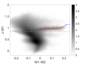
(a) Gaia/WISE/2MASS data.

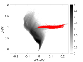
(b) Galaxia synthetic star population including cosmic scatter and extinction, but without photometric measurement scattering. M-dwarfs (see text) highlighted in red.

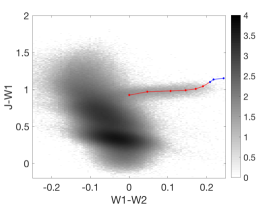
(c) Galaxia synthetic star population including cosmic scatter, extinction, and initial photometric measurement scattering.

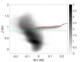
(d) Galaxia synthetic star population including cosmic scatter, extinction, and final photometric measurement scattering.

Figure 3: Logarithmic source densities in the J–W1/W1–W2 plane for sources with 9 < G < 14.5. Objects below the green horizontal line in the 3a and 3d are used to normalise Galaxia to observational data. The M-dwarf spectroscopic comparison sample from § 2.2 are overplotted in red and blue.

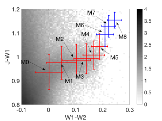
Figure 4: Galaxia generated colour-colour density in J–W1/W1–W2 expanded around the M-dwarf branch. Overplotted are points representing the median colour and r.m.s. for spectroscopically observed M-dwarfs (M0-M5 in red, M5-M8 in blue).

3.1 Photometric scatter

As noted above, scatter needs to be added to Galaxia’s simulated photometry to match the expected photometric uncertainties for our observational data – this is obvious from Figs. 3a and 3b, where we see the observed distribution is noticeably more scattered from the Galaxia one.

The observational data all come with estimated 1-$\sigma$ uncertainties, so we obtained uncertainty distribution functions for each observed bandpass by binning these uncertainties in 0.005 magnitude bins (for 2MASS/WISE) and 0.0002 magnitude bins (for Gaia) – see Figure 5 for an example.

For each simulated magnitude (e.g. $W1$), we then randomly drew from the appropriate distribution function for that magnitude bin, to obtain an estimate of the uncertainty for that simulated object (e.g. $\sigma_{W1}$). We then randomly drew from a normal distribution with that uncertainty to obtain a scattering estimate (e.g. $\Delta_{W1}$), which was applied to the simulated magnitude to obtain a scattered magnitude. Following the application of this suitable level of photometric scatter, our simulation was then trimmed to only contain simulated sources with G < 14.5.

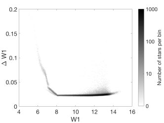
Figure 5: Density plot of the number of stars per bin of the WISE photometric uncertainty as a function of the WISE magnitude W1.

The result of this photometric scattering applied to the data of Figure 3b is shown in Figure 3c – the result is to significantly “over scatter” the simulated data compared to the observational data of Figure 3a. All the features in W1–W2 in the scattered simulated data are too broad, as is the width of the M-dwarf branch in the J–W1 direction. Since the aim of our simulations is (in the end) to create simulated data that looks like observational data, we empirically adjusted the fraction of the predicted photometric scatter applied to the simulated data, so as to matched the observed distribution. It was found our initial scattering needed to be reduced by a factor of near a half, and this is shown in Figure 3d.

3.2 Colour terms and offsets

Comparison of the simulated and scattered data with the observational data, showed small – but notable – colour differences between Galaxia predicted colours and observed colours at the level of several hundredths of magnitude to a few tenths of a magnitude. This is not entirely surprising, inasmuch as the Galaxia predicted colours rely entirely on synthetic model atmospheres and model filter profiles.

We therefore used “benchmark” features in the observed data, to align the two sets of data. Figure 6 shows example contours (rather than grey scales) of source density in J–W1/W1–W2 after these offsets were determined and applied. Offsets were determined using observed stars with G=9-14.5 from a number of features: the M-dwarf branch at J–W1$\approx$1; the G-dwarf clump at W1–W2$\approx$-0.03, J–W1$\approx$0.35; and the giant clump at W1–W2$\approx$-0.07, J–W1$\approx$0.7. Because the aim of this work is to understand how selection criteria for M-dwarfs will be influenced by contamination, these offsets were weighted more heavily on the features nearest to the M-dwarf branch, as these are the source most likely to contaminate our M-dwarf selection. This is why in Figure 6 the giant clump is better aligned than the G-dwarf clump. The offsets so determined and applied are reproduced in Table 2.

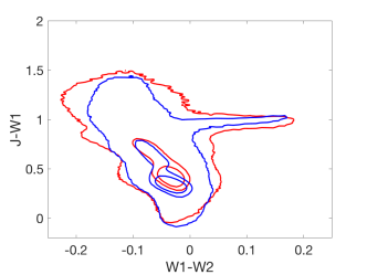
Figure 6: Contours containing 30%, 60% and 99% of the observational (in red) and simulated (in blue) data in J–W1, W1–W2. Offsets from Table 2 have been used to align the simulation M-dwarf branch to its observational counterpart.

G–J	G–H	G–K	G–W1	G–W2
-0.1	-0.25	-0.2	-0.3	-0.3
	J–H	J–K	J–W1	J–W2
	-0.01	-0.01	-0.03	-0.07
		H–K	H–W1	H–W2
		0	-0.02	-0.05
			K–W1	K–W2
			-0.04	-0.02
				W1–W2
				-0.025

Table 2: Zero-point colour offsets to align Galaxia colours with observed colours (in the sense that these offsets are added to synthetic colours).

3.3 Normalising Galaxia to the Sky

Each Galaxia simulation run produces an arbitrary number of stars (in this case 4,931,764). To compare this synthetic Galaxia population with the observational Gaia/WISE/2MASS data, we therefore need to estimate a normalisation between the two data sets. As noted above, while the colour offsets adopted (Table 2) aligned the M-dwarf branch, and features near that branch, in both datasets, there remain a number of differences.

As noted above the G-dwarf clump does not align in Figure 6, even after the M-dwarf and giant clumps are aligned. We believe this to be due to limits on the reliability of the synthetic photometry adopted by Galaxia. Even after aligning for colour offsets there clearly remain higher-order colour terms.

Another difference between the observed and simulated data is seen in the M-giant region at J–W1$>$1 (see Figure 3a and 3d). The real galaxy produces a plume of objects with a wide distribution of colours, while Galaxia simulates a much narrower range. This is likely to be due to the significant variability and mass-loss present in this class of stars, resulting in intrinsic reddening and scattering in colour that is highly variable from source to source. In this region the simulated data also contains fewer stars than the observational data.

Given these differences it was felt that normalising Galaxia to the Galaxy using the total number of objects in both samples would not be the best way to proceed. Instead we compared the types of stars best represented in both datasets. Galaxia has been heavily tuned to match the observed Galaxy for relatively unreddened G-K dwarfs and giants. We therefore normalised the two samples using the total number of stars 0.1 mag below the M-dwarf branch in each colour-colour space (shown by the green horizontal lines in Figures 3a and 3d), and adopted a normalisation factor of 1.211 to scale up the synthetic population to match the observational data. This means that, while the overall population will be close in number, specific regions may have differing numbers of stars.

4 Colour-colour selection

We have followed the long-standing tradition in giant-dwarf discrimination of selecting colour-colour diagrams which aim to break degeneracies between stellar effective temperature and surface gravity. Specifically, we seek colours sensitive to effective temperature for the horizontal axes, and sensitive to surface gravity for the vertical axes. Of course, no such diagram is perfect and contamination will occur where different classes of star overlap. Most notably for our case, the low-temperature boundary of the M-dwarf regime which adjoins the (much more numerous) high temperature boundary of the late K-dwarf regime, as well as the less numerous lower boundary of the K- and M-giants. Even small amounts of photometric scatter, cosmic scatter and source confusion in these more numerous populations will lead to significant contamination of any M-dwarf selection.

4.1 Connected Component Analysis

To aid in selecting colour-colour planes, we have made use of Connected Component Analysis (CCA; Samet & Tamminen 1988) to identify the colour regions spanned by key populations. CCA is a technique that identifies the pixels of a 2-dimensional image that comprise each component of the image. For our case, the images of interest are density images created by binning Galaxia simulated objects in colour-colour planes. Using this technique, we can select groups of components that comprise the majority of our sample, excluding highly scattered components that comprise a small fraction of the total population but would inflate our selected region, adding significant numbers of stars we do not intend to select (i.e. non-M-dwarfs). For example, Figure 7 shows an example use of this technique for a density image of our adopted Galaxia M-dwarfs in the G–K/K–W2 colour-colour plane. The green contour is a rough measure of the region bound by all the Galaxia M-dwarfs while the red contour uses CCA to select 99.5% of the M-dwarfs but excludes a number of the most photometrically scattered M-dwarfs. Losing 0.5% of the M-dwarfs in our sample is an acceptable sacrifice to reduce the selected region and avoid as many non-M-dwarfs as we can.

We therefore compiled a set of criteria (listed in Table 3) to identify Galaxia sources as M- or K-giants, or K-dwarfs (as well as the previously discussed criterion for M-dwarfs). We then used CCA to identify regions in our data that contain > 97% of each of these classes of object in our Galaxia simulations (see Figure 8).

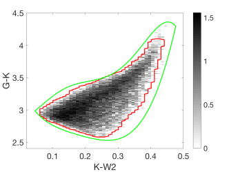
Figure 7: Connected component analysis of the Galaxia M-dwarfs using the G–K and K–W2 colours. The red outline highlights the region defined as the largest component while the green line represents the boundary region around the entire Galaxia M-dwarf population for this colour plane.

Sp. Type	log(g)	Age (Yr)	T (K)
M-dwarf	4.2 - 5.4	> 5 x 108	2250 - 3900
K-dwarf	4.2 - 5.4	> 5 x 108	3900 - 4600
M-giant	< 4.2	> 5 x 108	2250 - 3900
K-giant	< 4.2	> 5 x 108	3900 - 4600

Table 3: Stellar characteristics used to define the M and K, dwarf and giant populations in the synthetic Galaxia population.

4.2 Stellar distributions

After examining the many colour-colour combinations available to us from our six passbands, we selected three for use in our analysis. Each possesses distinct advantages.

G–K/K–W2: This plane displays the smallest levels of K-dwarf/M-dwarf overlap in all the colour-colour planes (Figure 8a). In all colour-colour planes, K-dwarfs are the most significant source of contamination in the M-dwarf region, so selecting a colour-colour space that minimises this overlap greatly lowers the overall level of contamination.

J–K/G–J: This plane has the advantage of using the G-band in the temperature-dependent horizontal axis (Figure 8b) to distribute the M-dwarf branch across a large colour range.

J–K/W1–W2: This has the advantage of using a colour on the horizontal axis for which both bands come from the same survey, telescope and instrument (Figure 8c), which reduces issues associated with cross-matching, and systematics between surveys with different sensitivities, instrument resolution and data processing.

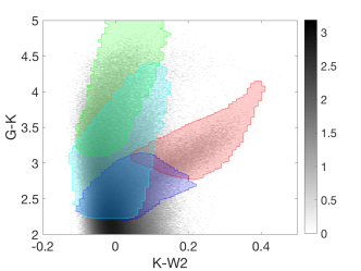
(a)

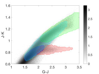
(b)

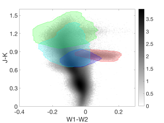
(c)

Figure 8: The three colour-colour spaces chosen for this work. Coloured regions highlighting the four classes of stars of importance to this work, as identified by the CCA analysis described in §4.1. In each case these connected regions contain > 98% of the relevant class in our Galaxia simulation. Red - M-dwarfs; Blue - K-dwarfs; Cyan - K-giants; Green - M-giants.

5 Analysis

We were guided by the principle of keeping our photometric selection criteria as simple as possible. We first experimented with simple rectangular selection regions in colour-colour space, bounded by the maxima and minima of the CCA regions for M-dwarfs. However, these were quickly found to be unsatisfactory – there was simply too much contamination at the boundaries between between classes of object, which do not follow either vertical or horizontal lines in these planes.

The next simplest model (i.e. parallelograms) were utilised as the simplest polygon able to represent the M-dwarf region. We binned the data in the M-dwarf CCA region along each horizontal axis and fitted a linear polynomial to the middle 60% of points in each bin. Figure 9 shows an example of this for the data plotted in Figure 7.

This results in the three groups of “high completeness” criteria shown in Equations LABEL:eqHC1-LABEL:eqHC3, which are shown in Figure 10 overplotted on our observational data as by the combined red and green parallelograms. We then require that an object must satisfy all three of these colour-colour criteria to be considered a candidate M-dwarf.

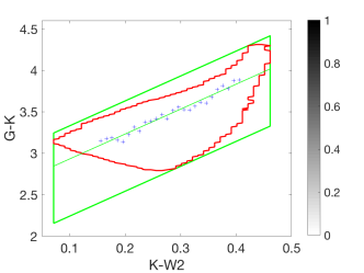
Figure 9: Construction of a parallelogram selection region using the CCA information seen in Figure 7. The red line bounds the primary connected component, the blue crosses represent the G-K values of highest density for the middle 60% of the K-W2 bins. The thin green line is a linear fit through the blue crosses and the thick green lines represent the parallelogram formed from the intersection of the polynomial with the minimum and maximum K–W2 values from the primary connected component.

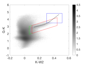
(a)

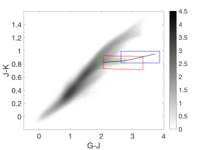
(b)

(c)

Figure 10: Colour-colour density plots of Gaia/WISE/2MASS photometry with the colour regions for the low contamination (in red) and high completeness (in green) criteria for G < 14.5. The blue box contains the M6-8 stars that are absent from our low contamination and high completeness colour regions. The black line represents the M-dwarf median colour values from Table 1.

$$\hskip 42.67912pt\begin{split}K-W2>0.061\\ K-W2<0.441\\ G-K>3.19(K-W2)+1.944\\ G-K<3.19(K-W2)+3.019\\ \end{split}$$ (1)

$$\hskip 42.67912pt\begin{split}G-J>1.911\\ G-J<3.331\\ J-K>-0.013(G-J)+0.732\\ J-K<-0.013(G-J)+0.929\\ \end{split}$$ (2)

$$\hskip 42.67912pt\begin{split}W1-W2>-0.069\\ W1-W2<0.221\\ J-K>-0.065(W1-W2)+0.731\\ J-K<-0.065(W1-W2)+0.949\\ \end{split}$$ (3)

While the completeness of this combined set of criteria is very high (99.3% – see Discussion), the number of simulated non-M-dwarfs significantly outnumbers the number of simulated M-dwarfs, with most of the non-M-dwarf contamination arising at the transition point from K-dwarfs/giants to M-dwarfs.

The conditions that define both sets of criteria consist of four colour limits per colour-colour plane. The most influential is the blue limit of the x-axis as this is where the transition point between K-stars and M-dwarfs occur. This limit will affect both the contamination levels, and what fraction of the total number of M-dwarfs (in particular, M0) are within our selected region. Moving this limit to bluer values will increase the number of M-dwarfs selected, but will add a substantial amount of K-stars. Reducing the size of the selected region by moving this limit to redder values will reduce the K-star contamination, at the expense of the M-dwarf completeness. The other three limits, while important, are not as crucial as the blue x-axis limit.

To lower this contamination rate we constructed a second set of “low contamination” criteria (Equations LABEL:eqLC1-LABEL:eqLC3), by moving the lower x-axis boundary conditions of each colour region to reduce the number of stars selected. The stars excluded from the colour region will include both M-dwarfs and non-M-dwarfs. The optimal colour region will exclude as many non-M-dwarfs as possible while minimising the amount of M-dwarfs that are lost. We decided to divide the x-axis range of each colour region by twenty, move the lower boundary condition in by that amount and determine the number of M-dwarfs and non-M-dwarfs in the selected region. This was calculated for all three colour spaces and all permeations. The optimal set of colour ranges by maximising the Equation 4, where $M_{tot}$ is the total number of stars identified in Galaxia as M-dwarfs, $M_{sel}$ is the number of Galaxia identified M-dwarfs within our selected colour region and $S_{sel}$ is the total number of stars within our selected colour region.

$$\hskip 85.35826ptf=\frac{M_{sel}}{M_{tot}}\times\frac{M_{sel}}{S_{sel}}$$ (4)

The low contamination criterion has non-M-dwarfs comprising $\approx$36% of the total selected sample, while maintaining M-dwarf completeness at $>$95%.

$$\hskip 42.67912pt\begin{split}K-W2>0.099\\ K-W2<0.441\\ G-K>3.19(K-W2)+2.045\\ G-K<3.19(K-W2)+3.140\\ \end{split}$$ (5)

$$\hskip 42.67912pt\begin{split}G-J>2.053\\ G-J<3.331\\ J-K>-0.013(G-J)+0.730\\ J-K<-0.013(G-J)+0.927\\ \end{split}$$ (6)

$$\hskip 31.2982pt\begin{split}W1-W2>-0.011\\ W1-W2<0.221\\ J-K>-0.065(W1-W2)+0.728\\ J-K<-0.065(W1-W2)+0.945\\ \end{split}$$ (7)

As noted earlier, we expect late M-dwarfs (i.e. later than M5 – shown in blue in Figure 4) to appear off the red end of the Galaxia M-dwarf branch, because Galaxia cannot simulate them. This can be seen from Figure 10 in which our observed M-dwarf photometric sequences are shown as the black curves. To select these late M-dwarfs would necessitate moving the “vertical” red cut-off in K–W2, G–J and W1–W2 in Equations LABEL:eqHC1-LABEL:eqHC3 and LABEL:eqLC1-LABEL:eqLC3 to a redder value, as well as also allowing slightly redder colours in G–K and J–K.

We expect the number of such very late M-dwarfs to be small. Nonetheless, we developed a supplementary selection criteria to cover the full M-dwarf range, using the median colours and r.m.s. scatter for M6-M8 spectroscopic comparison data (§2.2). As this area is far from the main sources of contamination (K-stars and giants) using a rectangle to bound this region is adequate, and these late M-dwarf colour regions are indicated by the blue boxes in Figure 10.

Selecting the full range of M-dwarfs requires the late M-dwarf criterion and either the high completeness or low contamination criterion. As such we define the “HiComp” criteria as Equations LABEL:eqHC1-LABEL:eqHC3 plus LABEL:eqLM1-LABEL:eqLM3 and the “LoCont” criteria as Equations LABEL:eqLC1-LABEL:eqLC3 plus LABEL:eqLM1-LABEL:eqLM3.

$$\hskip 85.35826pt\begin{split}K-W2>0.298\\ K-W2<0.508\\ G-K>3.493\\ G-K<4.823\\ \end{split}$$ (8)

$$\hskip 93.89418pt\begin{split}G-J>2.625\\ G-J<3.864\\ J-K>0.816\\ J-K<0.995\\ \end{split}$$ (9)

$$\hskip 82.51282pt\begin{split}W1-W2>0.150\\ W1-W2<0.268\\ \end{split}$$ (10)

6 Discussion

6.1 Colour Selection pre-Gaia DR2

6.1.1 Completeness and Contamination in Simulations

Our simulated data allow us to quantify both the completeness and contamination (i.e. the false-positive rate) for M-dwarf candidate selection using these criteria. We define simulated completeness as the number of M-dwarfs selected, divided by the total number of M-dwarfs present in the simulation, and simulated contamination as the number of non-M-dwarfs identified by each set of criteria, divided by the total number of object selected by each set of criteria. These results are reported in Table 4.

The HiComp criterion (Eqs LABEL:eqHC1-LABEL:eqHC3 and LABEL:eqLM1-LABEL:eqLM3) is designed to maximise the selection of M-dwarfs, at the cost of higher non-M-dwarf contamination. We predict that this criterion would select 99.3% of all M-dwarfs, at the cost of 55.6% of the objects selected not actually being M-dwarfs. Whether this level of contamination is acceptable for M-dwarf selection will depend greatly on the total number of candidates identified and the resources available for follow-up of those candidates. If the total number identified is $\sim$50,000 objects and they can be observed spectroscopy as part of a survey targeting 1,000,000 stars a year (as is the goal of the FunnelWeb survey), then the cost of a contamination rate of 55.6% is perfectly acceptable. If they are being followed-up by observation one-at-a-time, then that cost would be prohibitive.

The LoCont criterion (Eqs LABEL:eqLC1-LABEL:eqLC3 and LABEL:eqLM1-LABEL:eqLM3) reduces the number of M-dwarf candidates by about a third down to 37,079 giving a contamination rate of just 35.9%, at the cost of lowering M-dwarf completeness to 98% (i.e. missing  300 simulated M-dwarfs, almost all of which will be early M0 types).

6.1.2 Contamination in Observations

Applying the same selection criteria to our observational sample selects the number of objects that “Meet Criteria” listed in Table 4. The first point that is apparent from these numbers is that the number of observed objects that meet the HiComp criterion is around 44% higher than the number predicted by the Galaxia simulation – i.e. 78,340 vs 54,255. The corresponding difference for the LoCont sample is much smaller at 9.2% (40,505 vs 37,079).

As noted earlier (§3.3), it was found to be problematic to obtain a single normalisation between our Galaxia and observational data sets, with different regions of the simulated colour-colour plane requiring different normalisations. Our chosen overall normalisation was one based on the population of main sequence stars with J–W1 < 0.67, where Galaxia has been most tuned to accurately match the observed Galaxy.

There are two ways to look at the difference between the total number of objects selected by our criteria in our simulated data and in observed data. At one extreme, the number of simulated M-dwarfs could be correct and the simulations fail to reproduce the way the real world scatters non-M-dwarfs into the colour selection criteria regions. At the other extreme the simulations could be correctly predicting the total number of objects in the colour selection regions, and under-predicting the total M-dwarf stellar population – in this situation, our best estimate of the number of M-dwarfs to be identified will be the number of observed objects that meet our criteria, times one-minus-the-contamination-rate derived from our simulations. The fact that the difference between the predicted and observed number counts is significantly smaller for the LoCont sample (which digs into the K-dwarf, K-giant and M-giant regime much less than the HiComp sample) suggests the former is more likely. However we cannot rule out the latter.

We therefore provide in Table 4 two estimates for the total number of M-dwarfs predicted to be found in the observed sample. They are the extreme bounds that arise from these two assumptions. For the HiComp criterion the contamination rate range is 55.6-69.3%, while for the LoCont criterion it is 35.9-41.3%.

The key point here is that the total numbers of objects predicted ($\approx$78k and $\approx$40k for the two sets of criteria respectively) are both tractable numbers for a massively multiplexed, all-sky spectroscopic survey like FunnelWeb, where the cost to observe $\sim$100,000 objects a year is low, as the time scale is relatively short. In this situation, obtaining a highly complete spectroscopic sample becomes a clear priority.

6.1.3 Impact of the latest M-dwarfs

Galaxia (as noted earlier) cannot predict the number of late M-dwarfs we will find (or miss) for these photometric selection criteria. However, we can look at our observational data to at least estimate the scale of the problem.

If we look at the number of objects selected by Equations LABEL:eqHC1 - LABEL:eqHC3 plus LABEL:eqLM1 - LABEL:eqLM3 vs LABEL:eqHC1 - LABEL:eqHC3 alone we find 249 extra objects in our observational data that are potential late-M-dwarfs not captured by our early-M-dwarf criterion. (This number is the same for both the HiComp and LoCont criteria). As such, the inclusion of late M-dwarf candidates comes at almost no cost to the FunnelWeb survey, making their inclusion eminently sensible.

	Simulations				Observations
Criteria	Meet	Total	Completeness	Contamination	Meet	Predicted M-dwarfs
	Criteria	M-dwarfs	(%)	(%)	Criteria	(Number)	(%)
HiComp	54255	24078	99.3	55.6	78340	24078 - 34767	30.7 - 44.4
LoCont	37079	23764	98	35.9	40505	23764 - 25960	58.7 - 64.1

Table 4: Simulation and Observation predictions for M-dwarf selection using High Completeness (HiComp) and Low Contamination (LoCont) criteria. “Meet Criteria” numbers are all objects in either samples that meet the HC and LC criteria. The simulated “Total M-dwarf” numbers are simulated objects identified as M-dwarfs that are selected by each set of criteria, and “Completeness” is the percentage of that number of the total number of simulated M-dwarfs. “Contamination” is the percentage of simulated objects that “Meet Criteria” but are not simulated M-dwarfs. “Predicted M-dwarfs” are the extreme ranges for numbers of objects in the Observational sample that “Meet Criteria” and could be real M-dwarfs (see text).

6.2 Absolute Magnitude Selection post-Gaia DR2

In an ideal world, M-dwarf selection would be made on the basis of the one parameter that clearly distinguishes them from all other classes of stars – luminosity (with perhaps a simple colour selection required to distinguish degenerate white dwarfs from main sequence red dwarfs). Our exploration of M-dwarf selection using photometric colour criteria was primarily motivated by the desire to perform a kinematically unbiased selection for M-dwarfs in the absence of the distances required to make a purely absolute magnitude-limited selection.

However, with the release of Gaia DR2, international astronomy will enter into that “ideal” world. We have therefore used our simulated data to examine the impact of such a revolutionary set of complete, all-sky distance measurements.

We calculated the absolute magnitude M_G for all our simulated targets, and used them to construct a representative M_G:G–J colour-magnitude diagram (Figure 11a), and then used the characteristics from Table 3 and CCA techniques to identify and select the M and K dwarf, and M and K giant populations in this plane. It is clear that the issue of contamination of an M-dwarf sample by M and K giants is completely removed, and the only issue in such a plane is the degree of K dwarf contamination as a function of an adopted high luminosity limit in M_G for M-dwarfs.

Informed by these CCA regions, we have chosen two M_G cut-offs for M dwarf selection. A “high completeness” absolute magnitude (HiCompAbs) limit, and a “low contamination” absolute magnitude (LoContAbs) limit, as indicated in Equations LABEL:eqHiCompAbs andLABEL:eqLoContAbs and seen as the dashed and dotted black lines in Figure 11b.

$$\hskip 85.35826pt\begin{split}M_{G}>8.04\\ \end{split}$$ (11)

$$\hskip 85.35826pt\begin{split}M_{G}>8.86\\ \end{split}$$ (12)

These absolute magnitude limits were deliberately chosen to be analogous to our HiComp and LoCont colour selection criteria. Table 5 shows the same simulated completeness and contamination rates as shown for our colour selection criteria in Table 4. Using HiCompAbs M_G selection in isolation, significantly reduces the contamination rate of non-M-dwarfs (compared to the colour HiComp selection) by a factor of about 2. Moreover it does so while maintain M-dwarf completeness at 99.96%, a level higher than the HiComp criterion. Perhaps most critically, the HiCompAbs criterion selects more candidate M-dwarfs than the HiComp and LoCont colour selection criteria. (The LoContAbs selection would achieve an unacceptably poor level of completeness, so we do not consider it further).

Because the fraction of observed stars with pre-existing Gaia DR1 astrometry is so small ($\sim$12.5% of the stars in our Gaia/WISE/2MASS dataset have parallaxes from the Tycho-Gaia Astrometric Solution; Michalik et al. 2015), we are unable to compare these predictions with the real world in any meaningful fashion, until the release of Gaia DR2. Nonetheless it is both clear (and unsurprising) that precision distances will make a significant change in our ability to select M-dwarfs across the whole sky.

(a)

(b)

Figure 11: Simulated M_G:G–J colour magnitude diagram for G < 14.5. The K and M, dwarf and giant regions are identified using the criteria of Table 3, and the overplotted CCA regions (complete to > 97%) use the same colour scheme as in Figure 8. 11b is a zoomed in image of the K to M dwarf boundary seen in Figure 11a with black horizontal lines representing the absolute magnitude limits of HiCompAbs and LoContAbs.

	Simulations
Criteria	Meet	Total	Completeness	Contamination
	Criteria	M-dwarfs	(%)	(%)
HiCompAbs	34324	24247	99.96	29.4
LoContAbs	15963	13277	54.7	16.8

Table 5: Simulated predictions for M-dwarf selection using an absolute magnitude cut of M_G = 8.04 for HiCompAbs and M_G = 8.86 for LoContAbs.

6.3 Absolute Magnitude plus Colour Selection post-Gaia DR2

We now consider the impact of requiring both the colour and absolute magnitude criteria to jointly apply - i.e. the HiComp plus HiCompAbs criteria (hereafter, HiComp+), and the LoCont plus LoContAbs criteria (LoCont+). The results of such a selection are shown in Table 6 in the same format as Table 5.

	Simulations
Criteria	Meet	Total	Completeness	Contamination
	Criteria	M-dwarfs	(%)	(%)
HiComp+	32351	24068	99.2	25.6
LoCont+	15331	13083	53.9	14.7

Table 6: Simulated predictions for M-dwarf selection using the HiComp and LoCont colour criteria and an absolute magnitude cut of M_G = 8.04 for HiComp and M_G = 8.86 for LoCont.

The combination of all these criteria both completely removes contaminating giants from an M-dwarf candidate sample, and removes a substantial number of contaminating K-dwarfs. This can be seen more clearly in Figure 12, which compares the two sets of selections and how far they reach into the various contaminate star regions. The stars included in the HiComp selection but excluded from the HiComp+ selection (Figure 12b) are predominantly K-stars (cyan and blue), with a smaller amount of M-giants (green). The numbers of objects selected in Table 6 reinforce the idea that, once absolute magnitudes are available, the selection of a highly complete (i.e. $>$ 99%) M-dwarf sample becomes doable, with the requirement to follow-up a small number ($\approx$33k) of targets.

The LoCont+ (Figure 12a) selection excludes essentially all giants, with the contamination expected to consist of a small amount of K-dwarfs. However, this requires a selection limit so far into the M-dwarf branch to avoid the giant stars and this excludes a high amount of early M-dwarfs, dropping the completeness to just over 50%! Once again the low contamination option still has sufficient contamination and low enough completeness, as to not be worth utilising.

(a) HiComp v.s. HiComp+

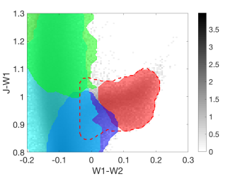
(b) LoCont v.s. LoCont+

Figure 12: The K-stars and M-giants plus the stars selected by our colour criteria and absolute magnitude cut. The dashed red contour represents the colour region selected by our colour criteria alone (i.e. HiComp and LoCont), while the red shaded area indicates the stars that are selected through colour and absolute magnitude (i.e. HiComp+ and LoCont+). The K-dwarf, K-giant and M-giant regions represent > 97% of their total respective populations and use the same colour scheme as Figure 8.

6.4 Comparison with the TESS Input Catalogue

We have cross-matched our identified HC candidates against version 5 of the TESS Input Catalogue (TIC; Stassun et al. 2017). The vast majority of our southern candidates are present in the TIC – we find only 234 HC sample stars that are not in the TIC. Details for these 234 objects are tabulated in Table LABEL:TabTIC, and overplotted in Figure 13. At the time of writing, the TIC does not contain any classification other than whether the object is a star, galaxy or is unknown. Additionally these 234 stars have no spectroscopy (and so no known spectral class) so we have used the empirical relationships between spectral type and photometric colours in Table 1 to estimate crude spectral types from each of their G–J, G–K, K–W2 and W1–W2 colours. (J–K was not used as the relationship is essentially flat for K7-M4 dwarfs, making it a very poor estimator for early M-dwarfs). As we saw in Figure 2, the accuracy with which we can estimate a star’s subtype is strongly dependent on the colour and subtype. W1–W2 and K–W2 type estimates are accurate to $\pm$2 subtypes, while G–J and G–K have similar accuracies for stars M5 and later, but are much more imprecise for earlier stars.

The mean of the four types indicated by these four colours is shown in Table LABEL:TabTIC, and is estimated to be good to $\pm$1.5 sub-types. All of these 234 candidates fall within the colour ranges expected for late K-dwarfs and early M-dwarfs, with approximately 70% of them expected to be early M-dwarfs (M0-M2 – see Table 7). The majority of these stars therefore fall within TESS’ target range for M-dwarf candidates of K5-M5.

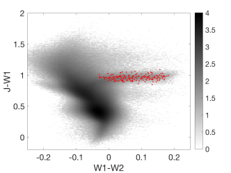
Figure 13: Colour-colour density plot of the observational Gaia/WISE/2MASS data and the stars that this work has identified as suitable candidates for the TIC, in red.

Subtype	#	%
K7	23	9.83
M0	73	31.20
M1	55	23.50
M2	36	15.38
M3	34	14.53
M4	13	5.56

Table 7: Distribution of approximate classifications for the 234 HiComp M-dwarf candidates not currently in the TESS Input Catalogue (version 5).

7 Conclusions

We have developed a set of criteria based on the comparison of synthetic and observational photometry. One criterion (HiComp) focusses on selecting as many M-dwarfs as possible, regardless of the levels of non-M-dwarfs. While the contamination levels in the HiComp criterion are not trivial, multi-star spectroscopic surveys, such as FunnelWeb will be able to observe all candidate stars in a relatively short period of time and spectroscopically confirm the M-dwarfs.

The other criterion (LoCont) is a subset of the first, that reduces the number of non-M-dwarfs, but in doing so, excludes significant levels of early M-dwarfs and as such, is most suitable as a list of high priority candidates on “one target at a time” spectroscopic surveys.

Once the Gaia DR2 is made publicly available, the best method for the identification of determine M-dwarfs will be to use the calculated distances and fluxes to determine luminosities. Our work shows that the rates of M-dwarf completeness and non-M-dwarf contamination are tractable with colour selection alone, but that absolute magnitude selection is even better. In the post-Gaia DR2 era, the combination of absolute magnitude and colour selection will maximise M-dwarf completeness and minimise contamination.

Appendix A Candidate M-dwarfs for the TESS Input Catalogue

$\alpha$ (deg)	$\delta$ (deg)	2MASS	Gaia	Sp. Type
IRCS 2000	IRCS 2000	Identifier	Identifier
1.4272	-64.1394	00054261-6408215	4901148088120955264	M1
1.4302	-61.1742	00054318-6110264	4905603858992341888	M4
1.4399	-60.988	00054565-6059161	4905658044300034560	M2
1.5429	-60.141	00061044-6008267	4905941168543855872	M0
1.5819	-65.8428	00061920-6550262	4899957901143352576	M0
1.6412	-62.8692	00063384-6252087	4904458889430313088	M3
1.6431	-48.7531	00063428-4845109	4977749791917230848	M2
1.7037	-52.9209	00064882-5255157	4972113145557887360	M1
1.7809	-48.9119	00070740-4854431	4976993087399245568	K7
1.8475	-48.1048	00072340-4806162	4977838886719223424	M1
1.8854	-50.7964	00073253-5047468	4973546221525747328	M3
1.9568	-48.1025	00074958-4806089	4977836137940154624	M0
3.1762	-61.0898	00124220-6105215	4904941162718314368	M3
3.2336	-60.2659	00125618-6015561	4905786206123597696	M1
3.2353	-60.9572	00125649-6057259	4904945766923326336	K7
3.2723	-65.0349	00130528-6502056	4900134853796249216	M3
4.3631	-48.5491	00172720-4832568	4977166707158065152	M0
4.3879	-50.5431	00173322-5032347	4973717367382150912	M4
4.3964	-48.976	00173503-4858329	4977083934547993088	M0
4.408	-50.8909	00173783-5053267	4972946575371823104	M0
4.4405	-52.3699	00174586-5222113	4972549754753146624	M1
4.4488	-51.325	00174762-5119305	4972873114251308544	M3
4.7228	-48.8425	00185323-4850334	4977092322618533760	K7
4.7238	-48.0782	00185351-4804411	4977373140465224320	M3
4.75	-53.4972	00185991-5329496	4924229379808453504	M3
4.7856	-50.6626	00190849-5039454	4972956093019404928	M2
7.9958	-65.2795	00315893-6516465	4708068795401419904	K7
8.1024	-62.7352	00322472-6244057	4900982714699954944	M2
8.1063	-63.9459	00322550-6356450	4900626919608813440	M1
8.153	-60.4865	00323683-6029093	4905178279272755328	M3
10.3337	-53.4419	00412002-5326301	4921838560492998656	M0
10.3402	-48.691	00412140-4841274	4974891680160836224	M0
10.3834	-50.6801	00413198-5040483	4926450668174245248	M0
10.3967	-51.5842	00413522-5135030	4925226980451860480	M1
10.4117	-48.3846	00413879-4823042	4975087599388566912	M4
10.4179	-53.9022	00414033-5354083	4921578594712789888	M4
10.4233	-52.2104	00414163-5212367	4924965468483283200	M0
15.0549	-52.1271	01001292-5207377	4928118111920062848	M4
15.1272	-48.6328	01003033-4837570	4932718296769306112	M0
15.1354	-50.7177	01003248-5043041	4928479198408685568	M2
15.1636	-51.2984	01003933-5117534	4928394845250181120	M1
15.1732	-52.6472	01004163-5238497	4927307256452253312	M0
15.3229	-50.3421	01011736-5020323	4931583944366769408	M0
15.5803	-52.7496	01021921-5244589	4927279047106419584	M1
15.6506	-49.0611	01023608-4903397	4931916993310921600	K7
15.666	-49.0829	01023983-4904584	4931916718433006208	K7
15.7416	-51.3862	01025798-5123102	4928293209144203392	M2
19.122	-12.4072	01162917-1224252	2468686385004236032	M0
19.1947	-13.2468	01164675-1314482	2456488506085006720	M1
20.069	-22.5014	01201653-2230056	5041704225777536256	M1
20.1538	-22.3158	01203689-2218558	5043210934664106240	M1
20.1576	-20.6735	01203786-2040243	2353358679086279936	M0
22.8801	-20.9531	01313111-2057110	5043681525640788096	K7
22.8953	-19.5922	01313484-1935319	5140088732388630912	M3
22.94	-19.1524	01314551-1909083	5140143742332938752	M3
22.9473	-20.0364	01314735-2002109	5043941388341847296	M1
22.9549	-18.2411	01314916-1814265	2450182738180156288	M0
22.9631	-19.0234	01315107-1901269	2449995821203070336	M2
32.4292	-19.6991	02094293-1941570	5137052465388099840	M2
32.4773	-23.5008	02095450-2330036	5121712663273501952	M4
32.5006	-20.9393	02100005-2056218	5124515662009719424	M1
32.5018	-23.7051	02100040-2342177	5121694005935485312	M1
32.5121	-23.3846	02100287-2323049	5123215730028042496	K7
32.5324	-23.3426	02100777-2320334	5123216107985469312	M0
292.2349	-40.6332	19285636-4037586	6737513101292418688	M0
292.271	-38.6745	19290498-3840268	6738700917446630272	M1
292.2753	-36.8704	19290608-3652135	6739515208886313344	M2
292.2754	-38.5691	19290609-3834083	6738703769304980480	M2
292.3554	-37.3357	19292529-3720085	6739211812396448128	M4
292.3861	-41.903	19293264-4154103	6665326692595038976	M2
292.3878	-36.6094	19293304-3636332	6739528196868604416	M0
292.4241	-41.2263	19294176-4113348	6737416275550709504	M0
292.4722	-40.9639	19295330-4057494	6737490939260444544	M1
292.4735	-38.846	19295360-3850453	6737944590885952768	M1
292.5026	-38.1511	19300061-3809038	6739102342271888384	M2
292.5376	-39.9457	19300904-3956442	6737814504918193536	K7
292.5599	-41.379	19301439-4122435	6737400160833990656	M1
292.5839	-35.9047	19302010-3554168	6739630657609761920	M1
292.5903	-37.5557	19302167-3733204	6739193155059715712	M3
292.6461	-40.7436	19303504-4044356	6737500525629064064	K7
298.3412	-66.0982	19532188-6605530	6428334245492474240	M3
298.3459	-67.7701	19532297-6746125	6426888490780555008	K7
298.3658	-70.0732	19532775-7004235	6423365792964956288	M1
299.8833	-75.5368	19593200-7532130	6366722596033434496	M2
299.8852	-75.7719	19593236-7546189	6366506095322532864	M1
299.9059	-72.2381	19593722-7214164	6422137878994211456	M0
300.7833	-75.8848	20030800-7553053	6366511902118845440	M0
300.8206	-74.3163	20031692-7418577	6367678105998927872	M0
300.8314	-77.7506	20031949-7745017	6362732983732674688	M0
300.8736	-77.4678	20032981-7728039	6362933129208830848	M1
301.3896	-76.3148	20053347-7618532	6366440880539147264	M4
301.3933	-76.5111	20053435-7630399	6363409771794337920	M0
301.4111	-77.6162	20053825-7736585	6362928799881750784	M2
301.4138	-74.5453	20053932-7432433	6366908860176040576	M2
301.5189	-73.7204	20060424-7343130	6367734009292578176	M1
301.6473	-75.5488	20063516-7532543	6366535610337681920	M3
302.1928	-72.2107	20084599-7212373	6374109836703866496	M0
302.1953	-76.7082	20084682-7642291	6363391350679444224	M1
302.2385	-74.3382	20085706-7420164	6366936588484228992	M0
302.3059	-77.5129	20091355-7730461	6363116751945430912	K7
302.4183	-74.038	20094033-7402161	6366960502862346880	M3
302.5245	-74.3815	20100587-7422532	6366932911993073536	M3
304.6379	-60.5984	20183298-6035541	6443135286909909888	M1
304.6475	-62.7926	20183509-6247325	6430655177098790656	K7
304.7004	-60.5843	20184817-6035034	6443135596147568128	M3
304.719	-60.7144	20185249-6042510	6443130648345117440	M1
304.7532	-63.9155	20190090-6354563	6429424136396604032	M1
304.7844	-62.0634	20190823-6203486	6430901742581953408	K7
304.8169	-64.5867	20191605-6435127	6429324527512107008	M0
305.24	-65.8169	20205748-6549005	6425930644355539328	M2
305.2912	-62.4559	20210991-6227212	6430689811718803200	M0
314.3116	-49.0623	20571473-4903441	6478282619200079232	M4
314.3173	-50.4745	20571611-5028284	6477958228910103808	M1
314.3259	-52.833	20571828-5249572	6476512577278555008	M2
314.4073	-49.6871	20573776-4941123	6478203042046301952	M2
314.4262	-51.3785	20574235-5122421	6477496262227666304	M1
314.4476	-48.2281	20574740-4813410	6481437289859831936	M0
314.5364	-47.9471	20580870-4756497	6481450380919437568	M0
314.5708	-51.7533	20581690-5145111	6476702346112930560	M3
314.5861	-53.3084	20582057-5318298	6476280236727791488	K7
314.6217	-48.2112	20582913-4812403	6481427119377283072	M2
316.3029	-72.238	21051269-7214174	6371848553602876544	M4
316.3569	-73.7044	21052563-7342170	6370019034972766464	M0
316.4069	-74.611	21053758-7436391	6369827926107617408	M2
316.5137	-72.9976	21060304-7259507	6370253299669186944	K7
316.5461	-76.5223	21061096-7631203	6368358153940497664	M0
316.6646	-47.9891	21063947-4759203	6479978718965033600	M0
316.6805	-51.2622	21064331-5115441	6477067521412743936	M0
316.6866	-50.8197	21064473-5049102	6477188124094148608	M0
316.7346	-52.3832	21065624-5222585	6476760070473571200	M1
316.7763	-75.8816	21070620-7552536	6368951890219260672	K7
316.7808	-73.9927	21070691-7359330	6369952308360570880	M1
316.8139	-71.9542	21071525-7157151	6371881470232372480	K7
316.8159	-53.9481	21071580-5356527	6464234159132043776	M2
316.8402	-74.6913	21072153-7441291	6369823424981789184	M4
317.0286	-77.0813	21080745-7704525	6368255658841466368	M1
320.8627	-53.1939	21232692-5311380	6463767931842885632	M0
320.8886	-53.9367	21233324-5356122	6463663340798479488	M1
320.8894	-48.2343	21233347-4814037	6479185490045244160	M2
320.8926	-51.4282	21233419-5125414	6466216166280290176	M1
320.9452	-50.6946	21234679-5041394	6466320929122308352	M1
320.9559	-51.9219	21234944-5155189	6466094670246298752	M0
321.0039	-49.0663	21240115-4903577	6467116838101821568	M3
321.2061	-52.3414	21244940-5220288	6465331162499653248	M2
321.2539	-48.6666	21250084-4839587	6467152576525084544	M0
321.2669	-48.1107	21250412-4806365	6479179545810551040	M1
321.2908	-49.5336	21250984-4932015	6466952495473971584	M2
321.3111	-49.8057	21251469-4948205	6466930024204871936	M3
328.0035	-55.9749	21520084-5558294	6460607694905782912	M2
328.0263	-57.2998	21520630-5717594	6412368099706810496	M3
328.0466	-58.1673	21521107-5810017	6410788994853191552	M0
328.1083	-56.9157	21522601-5654563	6412415035108541440	M0
328.1163	-54.9942	21522777-5459378	6461064095310355328	M3
328.1519	-59.1771	21523641-5910368	6410433646436042368	M4
329.507	-68.1416	21580169-6808291	6396979575481957120	M0
329.5357	-71.6042	21580856-7136142	6395170569617138432	M0
329.5857	-68.3825	21582074-6822579	6396200915090592128	M1
329.6402	-68.532	21583342-6831549	6396195451892479744	M0
329.6407	-66.5214	21583359-6631167	6398720068028753024	M0
329.655	-66.1242	21583727-6607269	6398734327320523136	K7
329.6812	-71.4807	21584337-7128496	6395172974797882240	M1
329.6981	-70.8107	21584735-7048373	6395349893091578752	M3
329.7707	-66.6126	21590490-6636446	6398705705658038528	M0
329.7858	-69.9769	21590848-6958366	6395961049757161344	M2
330.1614	-69.0818	22003858-6904533	6396119001474821760	M0
330.2304	-68.7882	22005521-6847171	6396176244799223680	M1
330.4793	-67.098	22015489-6705520	6398541053792541312	M0
330.4881	-71.1986	22015699-7111538	6395277050448923520	M1
330.537	-66.6793	22020880-6640449	6398657911261911424	M1
330.5536	-69.2018	22021296-6912047	6396114362910173312	M0
330.6095	-71.1017	22022638-7106059	6395283647515686912	M0
330.6627	-69.9695	22023900-6958097	6395777774913000320	M2
330.6635	-69.3764	22023917-6922349	6396006679490533376	M1
335.3967	-49.7882	22213517-4947174	6511861326356030848	M1
336.8746	-65.2209	22272993-6513154	6404240406674616064	K7
336.9533	-61.1955	22274878-6111420	6406886484485966080	M0
336.9718	-62.0438	22275317-6202378	6406730182035851264	M1
336.9988	-65.0326	22275990-6501555	6404337335496639744	M2
337.0117	-63.3252	22280284-6319295	6405015287494373888	M0
337.1341	-63.3473	22283209-6320500	6405014600299775104	M3
340.6016	-55.2521	22422438-5515075	6506614800465225472	M1
340.6102	-58.1029	22422639-5806105	6503681853198330496	M0
340.6805	-56.9029	22424330-5654099	6504255111073279232	M0
340.7324	-55.8439	22425580-5550380	6505822842855567616	M0
341.0083	-55.2843	22440202-5517029	6505866754601833856	M3
341.0891	-57.9258	22442136-5755325	6504046444382581760	M2
341.1703	-57.0863	22444083-5705103	6504201612960643968	M0
341.6358	-59.3226	22463257-5919213	6503361757875496576	M0
341.6797	-58.0314	22464302-5801532	6503860042801179008	M1
341.7704	-57.8642	22470480-5751503	6503884919251887744	M0
341.7823	-59.1236	22470768-5907245	6503370622688061952	M1
341.7848	-57.4271	22470830-5725368	6503994526817585408	M0
341.8669	-57.0766	22472806-5704359	6504006690164558848	K7
341.8883	-57.3651	22473318-5721536	6503993324226096896	M0
341.9262	-56.768	22474226-5646044	6504227554563443200	K7
342.058	-68.1123	22481380-6806438	6384974901371874432	M1
342.1365	-66.5186	22483252-6631068	6391929003179743104	M0
342.378	-70.7325	22493063-7043561	6384279769504059648	K7
342.3969	-71.6922	22493560-7141313	6383945002574051072	M1
342.4851	-67.4008	22495623-6724020	6391021184532789504	M2
342.486	-70.7009	22495615-7042016	6384278468128958976	M2
342.5915	-67.8699	22502187-6752114	6390987237110516608	M0
347.3385	-49.8243	23092119-4949276	6502996685655270912	M2
347.3927	-51.6803	23093427-5140489	6502361923849262720	M3
347.4289	-51.4388	23094284-5126190	6502394531241135360	M0
350.4223	-49.8661	23214120-4951580	6526074025972604928	M0
350.4737	-52.4363	23215367-5226106	6501389234015189376	M2
350.4806	-52.7099	23215540-5242347	6501290003090808064	M3
350.5158	-49.8138	23220373-4948491	6526074816248262528	M0
350.5873	-53.8697	23222079-5352097	6499715811677467136	M1
350.6396	-52.3549	23223349-5221174	6501395212609739008	M0
350.702	-52.7438	23224857-5244375	6501278492578447488	M3
350.7246	-50.56	23225391-5033358	6501965859144654848	M3
350.729	-51.6076	23225491-5136273	6501811343401430144	M1
350.9227	-52.3418	23234147-5220307	6501381365635183872	M3
350.9249	-50.1135	23234185-5006485	6526019978104413952	M0
350.9317	-48.3676	23234351-4822035	6526632784038094976	M2
350.9741	-49.2686	23235398-4916062	6526162021262815488	M2
351.0546	-53.536	23241303-5332101	6501040757548608256	M0
351.08	-50.0411	23241898-5002281	6526024071208077568	M4
351.1067	-51.3368	23242553-5120114	6501838899911227264	M0
351.1476	-48.5501	23243541-4832595	6526583477813492736	M3
351.1547	-53.0622	23243699-5303439	6501082435911615872	M3
351.1788	-49.5513	23244272-4933035	6526061450308772096	M3
351.2735	-48.492	23250545-4829313	6526584611684870656	M0
355.4655	-49.2922	23415167-4917321	6523162072506258688	M1
355.4769	-50.7695	23415465-5046097	6522600600021061632	M0
355.5223	-50.355	23420527-5021176	6523011164535166720	M3
358.7286	-56.0164	23545493-5600590	6496660371942814464	M1
358.8308	-54.0629	23551929-5403456	6497258987305153920	M3
358.8433	-55.2542	23552259-5515138	6497079938710683904	M0
358.8753	-54.7908	23553007-5447273	6497121479632474240	M1
358.877	-54.7158	23553034-5442571	6497123266338916096	M0
358.8936	-54.3689	23553433-5422074	6497227204546900736	M2

Table 8: Southern hemisphere M-dwarf candidates not currently in the TESS Input Catalogue. The spectral type was estimated using photometry from WISE and a set of classified stars from West et al. (2011) and Zhong et al. (2015).

References

- Bressan et al. (2012) Bressan A., Marigo P., Girardi L., Salasnich B., Dal Cero C., Rubele S., Nanni A., 2012, MNRAS, 427, 127
- Chen et al. (2014) Chen Y., Girardi L., Bressan A., Marigo P., Barbieri M., Kong X., 2014, MNRAS, 444, 2525
- Chen et al. (2015) Chen Y., Bressan A., Girardi L., Marigo P., Kong X., Lanza A., 2015, MNRAS, 452, 1068
- Chu & Cui (1996) Chu Y. Q., Cui X. Q., 1996, in Kaifu N., ed., Ground-Based Astronomy in Asia. p. 327
- Gaia Collaboration et al. (2016a) Gaia Collaboration et al., 2016a, A&A, 595, A1
- Gaia Collaboration et al. (2016b) Gaia Collaboration et al., 2016b, A&A, 595, A2
- Keller et al. (2007) Keller S. C., et al., 2007, Publications of the Astronomical Society of Australia, 24, 1
- Kopparapu (2013) Kopparapu R. K., 2013, ApJ, 767, L8
- Leggett et al. (2002) Leggett S. K., et al., 2002, ApJ, 564, 452
- Lépine & Gaidos (2011) Lépine S., Gaidos E., 2011, The Astronomical Journal, 142, 138
- Luyten (1922) Luyten W. J., 1922, Lick Observatory Bulletin, 10, 135
- Luyten (1979) Luyten W. J., 1979, LHS catalogue. A catalogue of stars with proper motions exceeding 0“5 annually
- Michalik et al. (2015) Michalik D., Lindegren L., Hobbs D., 2015, A&A, 574, A115
- Reid & Hawley (2005) Reid I. N., Hawley S. L., 2005, New Light on Dark Stars: Red Dwarfs, Low-Mass Stars, Brown Dwarfs. Springer Praxis Books, Praxis Publishing Ltd, Chichester, UK, Berlin, Heidelberg
- Ricker & MORE (2009) Ricker G. R., MORE 2009, in American Astronomical Society Meeting Abstracts #214. p. 729
- Ricker et al. (2015) Ricker G. R., et al., 2015, Journal of Astronomical Telescopes, Instruments, and Systems, 1, 014003
- Robin et al. (2003) Robin A. C., Reylé C., Derrière S., Picaud S., 2003, A&A, 409, 523
- Samet & Tamminen (1988) Samet H., Tamminen M., 1988, IEEE Trans. Pattern Anal. Mach. Intell., 10, 579
- Sharma et al. (2011) Sharma S., Bland-Hawthorn J., Johnston K. V., Binney J., 2011, Astrophysical Journal, 730, 3
- Skrutskie et al. (2006) Skrutskie M. F., et al., 2006, AJ, 131, 1163
- Stassun et al. (2017) Stassun K. G., et al., 2017, preprint, (arXiv:1706.00495)
- Tang et al. (2014) Tang J., Bressan A., Rosenfield P., Slemer A., Marigo P., Girardi L., Bianchi L., 2014, MNRAS, 445, 4287
- Tarter et al. (2007) Tarter J. C., et al., 2007, Astrobiology, 7, 30
- West et al. (2011) West A. A., et al., 2011, in Johns-Krull C., Browning M. K., West A. A., eds, Astronomical Society of the Pacific Conference Series Vol. 448, 16th Cambridge Workshop on Cool Stars, Stellar Systems, and the Sun. p. 1407 (arXiv:1012.3766)
- Wright et al. (2010) Wright E. L., et al., 2010, AJ, 140, 1868
- Zacharias et al. (2000) Zacharias N., Rafferty T. J., Zacharias M. I., 2000, in Manset N., Veillet C., Crabtree D., eds, Astronomical Society of the Pacific Conference Series Vol. 216, Astronomical Data Analysis Software and Systems IX. p. 427
- Zhong et al. (2015) Zhong J., et al., 2015, The Astronomical Journal, 150, 42